Probing the time-variation of the fine-structure constant: Results based on Si IV doublets from a UVES sample

We report a new constraint on the variation of the fine-structure constant based on the analysis of 15 Si iv doublets selected from a ESO-UVES sample. We find $\Delta\alpha/\alpha$  = ${(+0.15\pm 0.43)\times 10^{-5}}$ over a redshift range of ${1.59\leq z\leq 2.92}$ which is consistent with no variation in $\alpha$. This result represents a factor of three improvement on the constraint on $\Delta\alpha/\alpha$ based on Si iv doublets compared to the published results in the literature. The alkali doublet method used here avoids the implicit assumptions used in the many-multiplet method that chemical and ionization inhomogeneities are negligible and isotopic abundances are close to the terrestrial value.

1 Introduction

Some of the modern theories of fundamental physics, in particular SUSY GUT and Super-string theory, motivate experimental searches of possible variations in the fine-structure constant. Such theories require the existence of extra ‘compactified’ spatial dimensions and allow for the cosmological evolution of their scale size. As a result, these theories naturally predict the cosmological variation of fundamental constants in a 4-dimensional sub-space (Uzan 2003 and reference therein).

In the framework of the standard Big-bang model, quasar spectra can be used as an important tool to test the variation of the fine-structure constant, $\alpha=e^{2}/\hbar c$, by allowing one to measure its value at different redshifts. Bahcall, Sargent & Schmidt (1967) were the first to use the absorption lines of alkali-doublets seen in QSO spectra to constrain the variation of this quantity. Their analysis provided ${\Delta\alpha/\alpha}\equiv(\alpha_{z}-\alpha_{0})/\alpha_{0}=(-2\pm 5)\times 10^{-2}$ at a redshift $z$ $\sim$ 1.95. Here $\alpha_{0}$ refers to the value of the fine-structure constant on Earth and $\alpha_{\rm z}$ to its value at redshift $z$. Since then several authors have used the alkali-doublet method (AD method) to constrain the variation of $\alpha$ (Wolfe, Brown & Roberts 1976; Levshakov 1994; Potekhin & Varshalovich 1994; Cowie & Songaila, 1995; Varshalovich, Panchuk & Ivanchik, 1996; Varshalovich, Potekhin & Ivanchik 2000; Martinez, Vladilo & Bonifacio, 2003). The method is based on the fact that the separation between energy levels caused by fine-structure interactions is proportional to $\alpha^{4}$ with the leading term of energy level being proportional to $\alpha^{2}$. As a result, to a very high accuracy, the relative separation of a fine-structure doublet, $(\lambda_{2}-\lambda_{1})/\lambda=\Delta\lambda/\lambda$, will be proportional to $\alpha^{2}$. Here $\lambda_{1}$ and $\lambda_{2}$ are, respectively, the rest wavelength corresponding to transition ²S${}_{1/2}\rightarrow^{2}$P_3/2 and ²S${}_{1/2}\rightarrow^{2}$P_1/2 of the alkali-doublet and  $\lambda$ is the average value of $\lambda_{1}$ and $\lambda_{2}$. Varshalovich, Potekhin & Ivanchik (2000) give the following relation between $\Delta\alpha/\alpha$ and the values of ($\Delta\lambda/\lambda$) at redshifts 0 and $z$:

$$\frac{\Delta\alpha}{\alpha}=\frac{cr}{2}\leavevmode\nobreak\ \bigg{[}\frac{(\Delta\lambda/\lambda)_{z}}{(\Delta\lambda/\lambda)_{0}}-1\bigg{]},$$ (1)

where “$cr$”($\approx 1$) represents the higher order relativistic correction.

Actually, the dependence of rest wavelengths to the variation of $\alpha$ is parameterized using the fitting function given by Dzuba et al. (1999a)

$$\omega=\omega_{0}+q_{1}x+q_{2}y$$ (2)

Here $\omega_{0}$ and $\omega$ are, respectively, the vacuum wave number (in units of cm^-1) measured in the laboratory and in the absorption system at redshift $z$. $x$ and $y$ are the dimensionless numbers defined as $x=(\alpha_{z}/\alpha_{0})^{2}-1$ and $y=(\alpha_{z}/\alpha_{0})^{4}-1$. The sensitivity coefficients $q_{1}$ and $q_{2}$ are obtained using many-body relativistic calculations (see Dzuba et al. 1999a). For a given doublet and $\Delta\alpha/\alpha<<1$, Murphy et al. (2001) have shown that Eq. (2) reduces to Eq. (1) with,

$$cr\approx\frac{\delta q_{1}+\delta q_{2}}{\delta q_{1}+2\delta q_{2}}$$

The value of “$cr$” for Si iv is 0.8914 when using the $q$ coefficients as given in Table 2 (see below).

The AD method works with emission as well as absorption lines. However emission lines are usually broad as compared to absorption lines. As a result, the constraints obtained from emission lines are not as precise as those derived from absorption lines. Bahcall et al. (2004) have recently found $\Delta\alpha/\alpha$ = ${(0.7\pm 1.4)\times 10^{-4}}$ using O iii emission lines from QSOs. The most stringent constraint from alkali-doublet absorption lines has been obtained by Murphy et al. (2001), $\Delta\alpha/\alpha$ = ${(-0.5\pm 1.3)\times 10^{-5}}$, by analyzing a KECK/HIRES sample of 21 Si iv doublets observed along 8 QSO sight lines.

The generalization of this method known as the many-multiplet (MM) method (Dzuba et al. 1999b) makes use of a combination of transitions from different species. The sensitivity coefficients $q_{1}$ and $q_{2}$ of heavier elements are found to be an order of magnitude higher than those of lighter elements. As a result the MM method gives an order of magnitude better precision in the measurement of $\Delta\alpha/\alpha$. Application of MM method to KECK/HIRES data resulted in the measurement of $\Delta\alpha/\alpha$ = ${(-0.57\pm 0.10)\times 10^{-5}}$ over the redshift range $0.2\leq z\leq 3.7$ (Murphy et al. 2003). However our recent investigation (Srianand et al. 2004 and Chand et al. 2004) using very high quality UVES data and well defined selection criteria resulted instead in a null detection of $\Delta\alpha/\alpha$ ($\Delta\alpha/\alpha$ = ${(-0.06\pm 0.06)\times 10^{-5}}$) over the redshift range $0.4\leq z\leq 2.3$.

Table 1: List of Si iv doublets in our sample

QSO	$z_{em}$	$z_{abs}$	Comments
HE 1341$-$1020	2.135	1.915
		2.147	saturated
Q 0122$-$380	2.190	1.906
		1.969
		1.973
		1.975
PKS 0237$-$23	2.222	1.597∗
HE 0001$-$2340	2.263	2.183
Q 0109$-$3518		2.045	contaminated
HE 2217$-$2818	2.414	1.965	weak & blend
		2.186	blend
Q 0329$-$385	2.435	2.251	contaminated
HE 1158$-$1843	2.449	2.266	blend
HE 1347$-$2457	2.611	2.329
Q 0453$-$423	2.658	2.276	contaminated
		2.502	blend
PKS 0329$-$255	2.703	2.328	unstable
		2.454
		2.455
Q 0002$-$422	2.767	2.167∗
		2.301	contaminated
		2.464
HE 0151$-$4326	2.789	2.451
		2.493
HE 2347$-$4342	2.871	2.735	contaminated
HE 0940$-$1050	3.084	2.667	contaminated
		2.828
		2.830	unstable
		2.916	blend
PKS 2126$-$158	3.280	2.727	contaminated
		2.768	contaminated
		2.907	contaminated
Q 0420$-$388	3.117	3.087	broad
‘∗’ Si iv system below Ly$\alpha$ emission
but included in our sample (see text).
“contaminated” Si iv doublet with inconsistent
profiles due to contamination of absorption
lines from other systems.
“blend” the majority of the components
have separations less than the
individual $b$ values.
“unstable” Si iv doublet with unstable Voigt
profile fit.

However, these results based on the MM method hinge on two assumptions:(i) ionization and chemical homogeneity and (ii) isotopic abundances of Mg ii close to the terrestrial value. Even though these are reasonable assumptions one cannot completely rule out systematic biases induced by them in the analysis, especially when one is looking for very small effects. On the contrary one can completely avoid the assumption of homogeneity in the case of the AD method because, by construction, the two lines of the doublet must have the same profile (see also Quast et al. 2004). Also the effect of isotopic shifts is negligible in the case of Si iv doublets (see Section 3.4 of Murphy et al. 2001). Therefore it is important to increase the precision of $\Delta\alpha/\alpha$ measurements based on the AD method. This can be achieved by (a) increasing the S/N ratio and spectral resolution of the data used; (b) increasing the sample size. The S/N ratio of the data used by Murphy et al. (2001) is in the range 15-40 per pixel and the spectral resolution is $R\sim 34000$. In this paper our motivation is to improve the $\Delta\alpha/\alpha$   measurements by using the alkali doublets detected in our UVES data of higher S/N and resolution. Si iv is used instead of C iv because wavelengths are better known for Si iv (Griesman & Kling 2000; Petitjean & Aracil 2004a) and $q$ coefficients are larger (see Table 2).

The organization of the paper is as follows. In Section 2 we briefly describe our data sample and analysis. The importance of selection criteria is discussed in Section 3 and discussion of individual systems are given in Section 4. The results and overall discussion are presented in Section 5.

2 Data sample and analysis

2.1 Data sample

The data used in this study have been obtained with the Ultra-violet and Visible Echelle Spectrograph (UVES) mounted on the ESO Kuyen 8.2 m telescope at the Paranal observatory for the ESO-VLT Large Programme “Cosmic evolution of the intergalactic medium” (PI Jacqueline Bergeron). This data set corresponds to a homogeneous sample of 18 QSO lines of sight with a Lyman-$\alpha$ redshift range of 1.7 to 3.2. The detailed quantitative description of data calibration are presented in Aracil et al. (2003) and Chand et al. (2004, here after Paper I). Briefly, the data is reduced using the UVES pipeline. Addition of individual exposures is performed by a sliding window and weighting the signal by the errors in each pixel. The final S/N ratio is about 60-80 per pixel and the median resolution $R$ $\sim$ 45000. The continuum is fitted using an automated continuum fitting procedure (Aracil et al. 2003).

The Si iv systems detected in our data set are listed in Table LABEL:tablist. There are 31 Si iv systems redshifted beyond the Ly$\alpha$ emission line from the quasar. In addition, two systems, marked with an asterisk (*) in Table 1, falling in the Lyman-$\alpha$ forest have well defined narrow components and have therefore been incorporated in the sample.

Among the 31 systems (beyond the Ly$\alpha$ emission), 9 systems are not considered in the analysis because they are contaminated by other metal lines and/or atmospheric absorption. They are noted as “contaminated” in column 4 of Table LABEL:tablist. In addition, 4 other systems are rejected for the following reasons. One is completely saturated (“saturated” in Table LABEL:tablist) and one is a very broad system (“broad”). The profile of this broad system is spread over 350 km s^-1, and has a few bad pixels in the central part of the Si iv$\lambda$1402 line. The other two systems (marked with “unstable” in column 4 of Table LABEL:tablist) were rejected during the analysis as we found that the component structure of their best-fit is not stable (as discussed in Section 3.2). Thus from a total of 33 systems, we exclude 13 systems (9 contaminated, one saturated, one very broad and 2 systems having large uncertainties in the component structure) and are left with 20 systems.

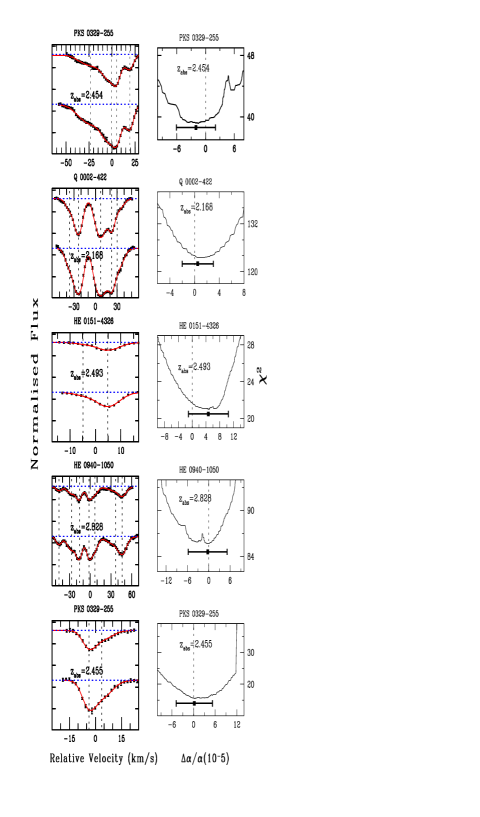
Figure 1: Left panels show on a velocity scale Si iv doublet data points with error-bars together with the best Voigt-profile fit for $\Delta\alpha/\alpha$ $=0$ over plotted as a solid curve. The dotted vertical lines mark the position of components. Right panels show the variation of $\chi^{2}$ as a function of $\Delta\alpha/\alpha$ for the systems in the corresponding left panel. Dark rectangles with error bar indicate the measured values of $\Delta\alpha/\alpha$ with one sigma error-bar obtained using $\chi^{2}_{min}+1$ statistics. Name of QSOs and $z_{\rm abs}$  are stated explicitly.

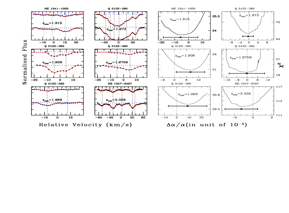
Figure 2: The first and second panels (from left) show on a velocity scale Si iv doublet data points with error-bars together with the best Voigt-profile fit for $\Delta\alpha/\alpha$ $=0$ over plotted as a solid curve. The dotted vertical lines mark the position of components. The third and forth panels show respectively the variation of $\chi^{2}$ as a function of $\Delta\alpha/\alpha$ for the systems in the first and second panels. Dark rectangles with error bar indicate the measured values of $\Delta\alpha/\alpha$ with the one sigma error-bar obtained using $\chi^{2}_{min}+1$ statistics. Name of QSOs and $z_{\rm abs}$  are also stated.

We have shown in Paper I (using detailed simulations) that it is better to avoid weak, or heavily saturated, or strongly blended absorption lines in order to obtain a better accuracy on $\Delta\alpha/\alpha$   measurements. Indeed, such systems can induce false alarm detection of non-zero $\Delta\alpha/\alpha$ .

Table 2: Atomic data of Si iv doublet used in our analysis:

Ion	$\lambda^{a}$(Å)	$\omega_{0}(cm^{-1})$	$q_{1}^{b}$	$q_{2}$	$f^{c}$
			$(cm^{-1})$	$(cm^{-1})$
Si iv	1393.76018(4)	71748.355(2)	$766$	$48$	0.5140
Si iv	1402.77291(4)	71287.376(2)	$362$	$-8$	0.2553
(a) Griesmann U. & Kling R. (2000)
(b) Dzuba et al. (1999a)
(c) Martin & Zalubas (1983) and Kelly (1987)

For a typical S/N ratio of 70 and a median $b$ Doppler parameter of 9 km s^-1  as seen in our sample, we define a lower limit for $N$(Si iv) of $1.55\times 10^{12}$ cm^-2 so that both lines of the doublets are detected at more than 5$\sigma$ level. As in Paper I, we define a multi-component system to be unblended if the majority of its components have separations larger than the individual $b$ values. We apply these criteria after the Voigt profile decomposition of the doublets (as described in the following Section). Based on the best fitted parameters, we decide whether a given system satisfies our selection criteria or not. Out of 20 systems for which we have performed Voigt profile fitting, 4 systems are blended and one system is both blended and weak. We mark these system respectively by ‘blend’ and ‘weak’ in column 4 of Table LABEL:tablist. As a result we are finally left with 15 Si iv doublets that are useful for $\Delta\alpha/\alpha$   measurements. The procedure used for the $\Delta\alpha/\alpha$ measurement is described in the next section.

2.2 Analysis

We first carry out a Voigt profile fit for each system assuming $\Delta\alpha/\alpha$ $=0$. The rest wavelengths for the Si iv doublet as well as the other atomic parameter used in the fits are summarized in Table 2.

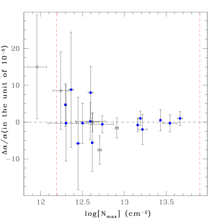
Figure 3: The figure shows $\Delta\alpha/\alpha$ measured from the 20 Si iv systems in our sample versus the column density of the strongest component in the system. Open circles are for systems that we define as ”blended” (they do not pass our selection criteria) and filled circles are for systems that pass this selection criteria. It is apparent that errors are larger for weaker systems and for blended systems as expected from the simulations presented in Paper I. The vertical dashed lines refer to the lower and upper cut off in column density to avoid very weak and heavily saturated systems.

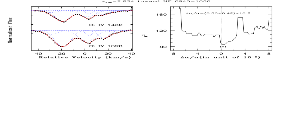
Figure 4: The left panel shows the Voigt profile best-fit to the system (solid line) along with sub-components profile (dashed lines). The right panel shows the variation of the $\chi^{2}$ as a function of $\Delta\alpha/\alpha$ . The $\chi^{2}$ curve is median smoothed over a smoothing scale of $1\times 10^{-5}$. The large fluctuation in the curve show that the minima is local and as a result the system is not considered in the final result. Note that the instability of the fit mainly comes from the poorly constrained structure of the central feature at $\sim$5 km s^-1.

The Voigt profile fit is carried out by simultaneously varying the column density, $N$, Doppler parameter, $b$, and redshift, $z$, for each component till the reduced $\chi^{2}$ of the fit is $\sim 1$. This gives us the required number of components to be used in the fit and an initial guess of $N$, $b$ and $z$ for each component.

To constrain the variation of $\alpha$, we use the analytical expression of the wave number ($\omega$) as a function of $\alpha_{z}/\alpha_{0}$ given by Dzuba et al. (1999a),

$$\omega=\omega_{0}+q_{1}\bigg{[}\bigg{(}\frac{\alpha_{z}}{\alpha_{0}}\bigg{)}^{2}-1\bigg{]}+q_{2}\bigg{[}\bigg{(}\frac{\alpha_{z}}{\alpha_{0}}\bigg{)}^{4}-1\bigg{]}.$$ (3)

The sensitivity coefficients $q_{1}$ and $q_{2}$, laboratory wave numbers ($\omega_{0}$) and rest wavelengths ($\lambda$) are listed in Table 2. The oscillator strengths ($f$) used in the analysis are given in the last column.

We then consider a change in $\Delta\alpha/\alpha$ and fit the system using the new rest wavelengths as given in Eq.(3). We vary $\Delta\alpha/\alpha$   from $-20.0\times 10^{-5}$ to $20.0\times 10^{-5}$ in steps of $0.1\times 10^{-5}$ and minimize $\chi^{2}$ for each value $\Delta\alpha/\alpha$ by varying N, b, and z. The value of $\Delta\alpha/\alpha$ at which $\chi^{2}$ is minimum ($\chi^{2}_{\rm min}$) is accepted as the measured value of the $\Delta\alpha/\alpha$ from the system, provided the reduced $\chi^{2}$ of the fit is also $\sim 1$. The n$\sigma$ error is obtain from value of $\Delta\alpha/\alpha$   where $\Delta\chi^{2}=\chi^{2}-\chi^{2}_{\rm min}=n^{2}$, assuming the error on data are normally distributed (Press et al. 2000, p. 691, Theorem D and Appendix A). To be on the conservative side we use as 1$\sigma$ error-bar, the larger of the two values of $\Delta\alpha/\alpha$ derived using $\chi^{2}-\chi^{2}_{\rm min}$ = 1 from the left and right side of $\chi^{2}_{\rm min}$. More details about the validation of our fitting procedure using the simulated data set can be found in Paper I.

In principle we can explicitly use $\Delta\alpha/\alpha$ as one of the fitting parameters (like $N$, $b$ and $z$) in our $\chi^{2}$ minimization. However in that case we will have no way of ensuring whether the best fitted value of $\Delta\alpha/\alpha$ is a true value or an artifact of local minima due to inconsistent fitting of the line profiles. Therefore to ensure that the $\chi^{2}$ minima with respect to our crucial parameter $\Delta\alpha/\alpha$ is not a local minimum, we have preferred to use the $\chi^{2}$ versus $\Delta\alpha/\alpha$ curve method rather than a single minimization that would simultaneously vary all four parameters, $\Delta\alpha/\alpha$ , $N$, $b$ and $z$. On the contrary, we minimize $\chi^{2}$ by varying $N$, $b$ and $z$ for each value of $\Delta\alpha/\alpha$ . We then determine the minima of the $\chi^{2}$ versus $\Delta\alpha/\alpha$ curve. Note that the two methods are equivalent as shown by Press et al. (2000, p. 691). For the sake of completeness we give details in Appendix A.

The Voigt profile fits to 11 individual systems and the corresponding plots giving $\chi^{2}$ as a function of $\Delta\alpha/\alpha$ are presented in Fig. 1 and 2. The Voigt profile fits to the other four systems, resulting in much more precise measurements of $\Delta\alpha/\alpha$ , are presented in more detail in Fig. 5 and Fig. 6 (see Sect. 4). The $\chi^{2}$ curves presented for all the systems are median smoothed over $\Delta\alpha/\alpha$ $=0.9\times 10^{-5}$, to avoid the obvious local fluctuations caused by one or two points in the curve. Since the smoothing scale we use is about one-half of the limiting accuracy from individual Si iv doublets, the final result is not affected by the procedure. The results of the Voigt profile fits are summarized in Table 3. In this table, Cols. 1 and 2 give the QSOs name and the emission redshift ($z_{\rm em}$). Cols. 3, 4 and 5 give, respectively, the mean absorption redshift (z̄_abs) of all the components in the system, the measured $\Delta\alpha/\alpha$ value and the reduced $\chi^{2}$ of the best-fit. The description regarding the component structure is provided in columns 6 to 9. In column 6 gives $z_{\rm abs}$  for individual components, while Cols. 7 and 8 respectively list the column density and velocity dispersion. Column 9 refers to the velocity of individual components relative to z̄_abs (listed in column 3).

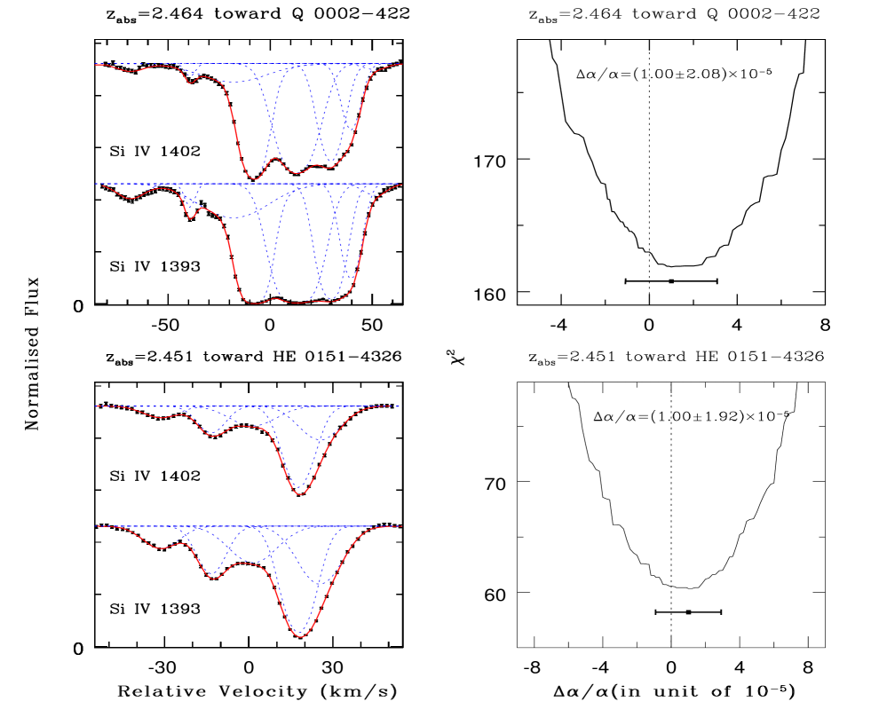
Figure 5: Left panels shows on a velocity scale Si iv doublet data points with error-bars together with the best Voigt-profile fit for $\Delta\alpha/\alpha$ $=0$ over plotted as a solid line. The Voigt profiles of individual sub-components are shown by dashed lines. Right panels show the variation of $\chi^{2}$ as a function of $\Delta\alpha/\alpha$ . The dark rectangle with error bars indicates the measured value of $\Delta\alpha/\alpha$ with one sigma error-bars derived using the criteria $\Delta\chi^{2}=1$ around the minima. The name of QSOs, $z_{\rm abs}$  and the value of measured $\Delta\alpha/\alpha$   are also stated explicitly.

In the course of the analysis we also noticed a few systems having weak components on the edge of stronger components (a specific example is discussed in Sect. 4.1). The parameters ($N$, $b$, $z$) of the weak components are difficult to constrain from an overall fit. We therefore froze alternatively one of the parameters (among $N$, $b$ and $z$) of the weak component and found that the final $\Delta\alpha/\alpha$ does not depend much on the choice of the frozen parameter. To be on the conservative side we have taken as the final error the largest error of all determinations. Such systems have zero errors for the corresponding frozen parameter in Table 3.

3 Importance of the selection

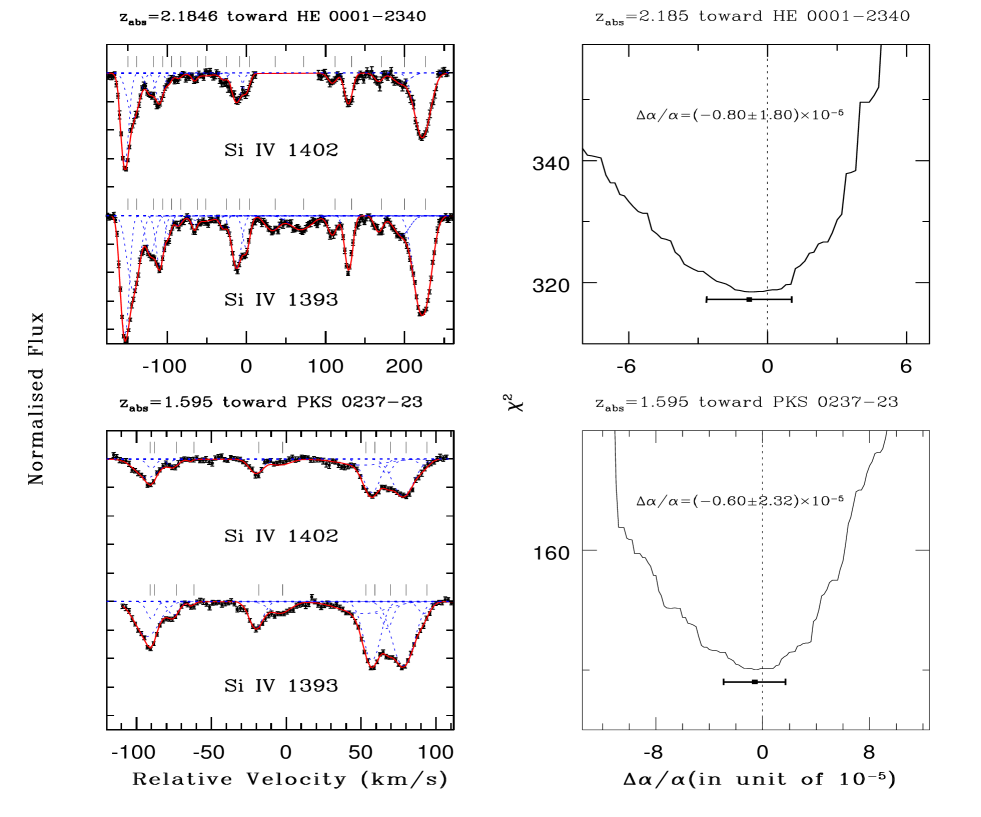
Figure 6: Same as Fig. 5. In addition, the position of sub-components is also marked by tick marks.

3.1 Errors versus strength of the absorption

As an illustration of the importance of the selection of the systems, we plot in Fig. 3 $\Delta\alpha/\alpha$ measured from the 20 Si iv systems in our sample versus the column density of the strongest component in the system. Open circles are for systems that we define as ”blended” (they do not pass our selection criteria) and filled circles are for systems that pass this selection criteria. It is apparent that errors are larger for weaker systems and for blended systems as expected from the simulations presented in Paper I. The column density of the strongest component is considered rather than the total column density since the precision in $\Delta\alpha/\alpha$  measurements is most often dominated by the strongest component.

3.2 Precise measurement versus local minima

We illustrate here the importance of the selection criteria with an example of a spurious precise measurement which results from local minima caused by an unstable fit. This happens in the rejected system at $z_{\rm abs}$= 2.8347 system toward HE 0940$-$1050. The Voigt profile best-fit (along with the profile of sub-components) and the variation of $\chi^{2}$ as a function of $\Delta\alpha/\alpha$ for this system are shown, respectively, in the left and right panels of Fig. 4. The system is fitted with 5 components and $\chi^{2}_{\nu}=0.97$. The right panel of Fig. 4 shows that the curve giving $\chi^{2}$ for this system possesses a large local fluctuation. The cause of such fluctuation is that the fit is unstable, either due to the uncertainty in the overall component structure or to abnormal fluctuation in a few pixels (see Fig. 4 around $v=17$ km s^-1 in Si iv$\lambda$1402 ). The uncertainty on the measurement as derived from this curve using our procedure would be underestimated. This kind of measurement could eventually dominate the whole statistics of weighted mean in the final result. It is important to mention that if we had not used the $\chi^{2}$ versus $\Delta\alpha/\alpha$ method, we may have considered this local minimum as a true minimum (Fig. 4).

4 Notes on individual systems

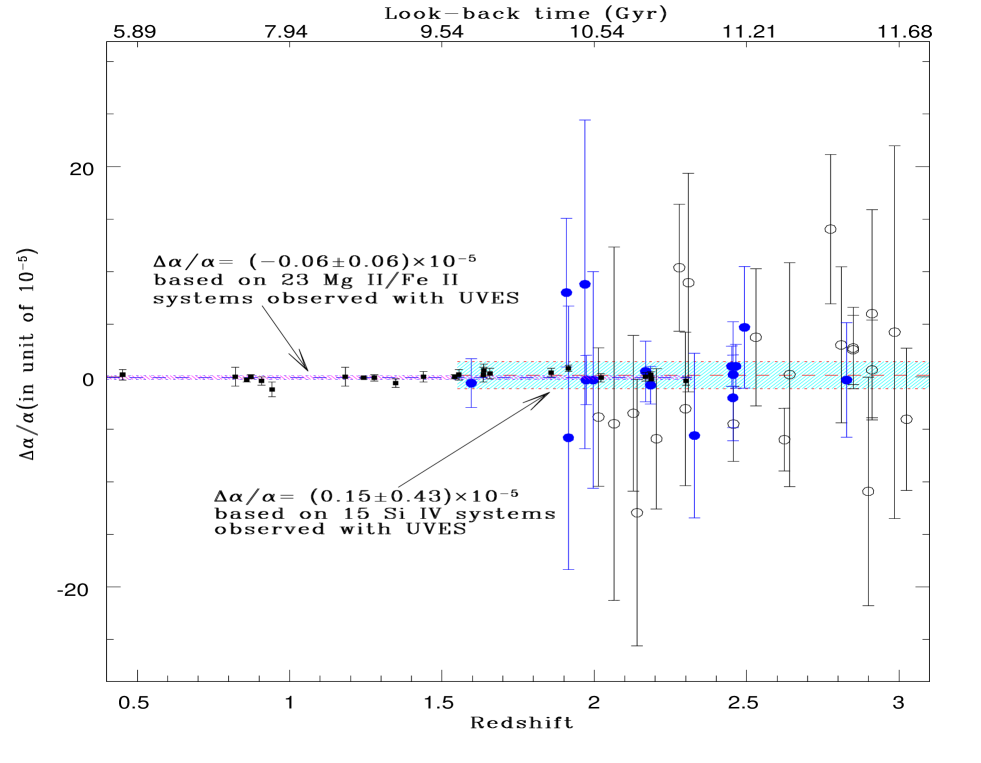
Figure 7: Measured values of $\Delta\alpha/\alpha$ versus the absorption redshift of the systems. The squares show our determinations from the MM method using Mg ii/ Fe ii systems and the narrow shaded region represents the 3$\sigma$ allowed range. The filled circles are our present measurements using Si iv doublets from UVES and open circles are the measurements from KECK/HIRES data by Murphy et al. (2001). The weighted mean from our 15 systems is ${\Delta\alpha/\alpha}$ = ${(0.15\pm 0.43)\times 10^{-5}}$. The $3\sigma$ allowed range ($-1.14\times 10^{-5}\leq\Delta\alpha/\alpha\leq 1.44\times 10^{-5}$) is shown by the wider shaded region.

Table 3: Results of the Voigt profile fits to the 15 Si iv systems those satisfy our selection criteria.

Name	$z_{\rm em}$	z̄abs	$\Delta\alpha/\alpha$	$\chi^{2}_{\nu}$	Component Structure
		(mean)	(in units of $10^{-5}$)		$z_{\rm abs}$	log10(N) cm-2	b(km s-1)	V(km s-1)
HE 1341$-$1020	2.135	1.91534	$-5.80\pm$12.54	0.44	$1.915491\pm 0.000800$	$12.447\pm 0.023$	$8.669\pm 0.632$	$15.530$
					$1.915210\pm 0.003547$	$11.799\pm 0.145$	$5.279\pm 2.652$	$-13.383$
					$1.915319\pm 0.002501$	$11.751\pm 0.162$	$3.333\pm 2.404$	$-2.171$
Q 0122$-$380	2.190	1.90870	$8.00\pm 7.08$	0.80	$1.908656\pm 0.000725$	$12.597\pm 0.027$	$2.651\pm 0.561$	$-4.586$
					$1.908745\pm 0.000940$	$12.400\pm 0.042$	$2.863\pm 0.867$	$4.598$
		1.96961	$8.80\pm 15.64$	0.52	$1.969496\pm 0.000963$	$12.364\pm 0.026$	$8.185\pm 0.715$	$-11.766$
					$1.969729\pm 0.003927$	$11.851\pm 0.098$	$9.433\pm 2.975$	$11.766$
		1.97337	$-0.30\pm 2.34$	0.87	$1.973533\pm 0.001488$	$13.188\pm 0.028$	$11.869\pm 0.000$	$16.779$
					$1.973729\pm 0.000358$	$12.547\pm 0.021$	$3.191\pm 0.326$	$36.552$
					$1.973096\pm 0.001843$	$12.730\pm 0.050$	$7.905\pm 0.873$	$-27.315$
					$1.973275\pm 0.001371$	$13.207\pm 0.186$	$4.122\pm 1.780$	$-9.261$
					$1.973192\pm 0.001700$	$12.922\pm 0.114$	$2.735\pm 0.841$	$-17.633$
					$1.973377\pm 0.002469$	$13.543\pm 0.083$	$8.025\pm 1.193$	$1.034$
		1.97587	$-0.30\pm 10.30$	0.58	$1.975917\pm 0.002038$	$12.303\pm 0.214$	$4.522\pm 1.177$	$4.711$
					$1.975823\pm 0.012910$	$12.064\pm 0.374$	$8.132\pm 5.132$	$-4.759$
PKS 0237$-$23	2.223	1.59671	$-0.60\pm 2.32$	0.82	$1.595925\pm 0.001055$	$11.763\pm 0.098$	$1.160\pm 2.414$	$-90.264$
					$1.595902\pm 0.001960$	$12.464\pm 0.060$	$10.260\pm 0.851$	$-92.922$
					$1.596053\pm 0.001286$	$11.703\pm 0.112$	$3.052\pm 1.549$	$-75.473$
					$1.597202\pm 0.000911$	$12.582\pm 0.159$	$6.297\pm 1.082$	$57.265$
					$1.597384\pm 0.001517$	$12.736\pm 0.136$	$8.762\pm 1.948$	$78.296$
					$1.597151\pm 0.048581$	$12.253\pm 0.704$	$21.079\pm 15.835$	$51.385$
					$1.597293\pm 0.001307$	$11.873\pm 0.256$	$1.650\pm 2.934$	$67.788$
					$1.597504\pm 0.003343$	$11.676\pm 0.357$	$3.785\pm 2.695$	$92.165$
					$1.596531\pm 0.000759$	$12.104\pm 0.041$	$4.919\pm 0.704$	$-20.245$
					$1.596669\pm 0.002426$	$11.898\pm 0.077$	$8.786\pm 2.127$	$-4.311$
					$1.596154\pm 0.000337$	$11.013\pm 0.202$	$0.276\pm 0.128$	$-63.807$
HE 0001$-$2340	2.263	2.18469	$-0.80\pm 1.80$	1.14	$2.183055\pm 0.000661$	$13.121\pm 0.063$	$4.817\pm 0.352$	$-153.733$
					$2.183171\pm 0.004262$	$12.855\pm 0.133$	$9.143\pm 2.517$	$-142.796$
					$2.183524\pm 0.002198$	$12.453\pm 0.184$	$5.042\pm 2.232$	$-109.556$
					$2.183398\pm 0.004220$	$12.367\pm 0.224$	$6.609\pm 3.394$	$-121.415$
					$2.183642\pm 0.002869$	$11.853\pm 0.231$	$2.758\pm 3.389$	$-98.439$
					$2.183769\pm 0.003596$	$11.654\pm 0.212$	$4.851\pm 3.711$	$-86.468$
					$2.184555\pm 0.001184$	$12.534\pm 0.046$	$6.542\pm 0.987$	$-12.420$
					$2.184685\pm 0.001782$	$12.204\pm 0.084$	$4.511\pm 0.993$	$-0.180$
					$2.184380\pm 0.002295$	$11.676\pm 0.147$	$3.821\pm 2.283$	$-28.905$
					$2.186058\pm 0.000353$	$12.502\pm 0.012$	$5.220\pm 0.268$	$129.163$
					$2.185840\pm 0.001094$	$12.021\pm 0.035$	$6.257\pm 0.893$	$108.613$
					$2.187051\pm 0.000462$	$13.158\pm 0.008$	$12.018\pm 0.230$	$222.706$
					$2.186770\pm 0.003257$	$12.290\pm 0.062$	$13.227\pm 2.068$	$196.226$
					$2.186462\pm 0.001357$	$11.922\pm 0.044$	$5.964\pm 0.965$	$167.209$
					$2.183988\pm 0.002104$	$11.575\pm 0.219$	$0.739\pm 1.589$	$-65.828$
					$2.185035\pm 0.002420$	$12.100\pm 0.052$	$11.632\pm 1.599$	$32.790$
					$2.185417\pm 0.003240$	$12.276\pm 0.044$	$18.832\pm 2.403$	$68.770$
					$2.184102\pm 0.011745$	$11.914\pm 0.148$	$20.314\pm 7.976$	$-55.092$
HE 1347$-$2457	2.611	2.32918	$-5.60\pm 7.84$	0.98	$2.328624\pm 0.001374$	$12.286\pm 0.029$	$10.056\pm 0.985$	$-50.424$
					$2.328948\pm 0.000556$	$12.616\pm 0.014$	$8.712\pm 0.410$	$-21.227$
					$2.329217\pm 0.001300$	$12.111\pm 0.040$	$7.045\pm 0.970$	$3.008$
					$2.329599\pm 0.003715$	$12.338\pm 0.058$	$16.509\pm 1.703$	$37.426$
					$2.329531\pm 0.000592$	$12.281\pm 0.050$	$3.913\pm 0.611$	$31.303$
PKS 0329$-$255	2.685	2.45465	$-2.00\pm 4.07$	0.47	$2.454707\pm 0.001053$	$12.579\pm 0.149$	$3.141\pm 1.277$	$4.886$
					$2.454874\pm 0.001173$	$12.542\pm 0.062$	$4.178\pm 0.598$	$19.400$
					$2.454643\pm 0.002560$	$13.215\pm 0.056$	$11.463\pm 0.896$	$-0.663$
					$2.454378\pm 0.004649$	$12.868\pm 0.065$	$16.186\pm 1.530$	$-23.686$
		2.45573	$0.20\pm 5.03$	0.36	$2.455683\pm 0.001245$	$12.593\pm 0.177$	$3.340\pm 0.913$	$-3.705$
					$2.455768\pm 0.007809$	$12.496\pm 0.236$	$7.026\pm 2.405$	$3.684$
Q 0002$-$422	2.760	2.16816	$0.50\pm 2.89$	1.33	$2.167774\pm 0.000928$	$12.509\pm 0.028$	$6.464\pm 0.000$	$-36.100$
					$2.167906\pm 0.000245$	$13.265\pm 0.007$	$6.198\pm 0.128$	$-23.592$
					$2.168234\pm 0.000308$	$13.430\pm 0.006$	$8.496\pm 0.164$	$7.473$
					$2.168391\pm 0.000357$	$12.985\pm 0.026$	$4.172\pm 0.327$	$22.328$
					$2.168473\pm 0.001424$	$12.750\pm 0.039$	$9.784\pm 0.000$	$30.094$
		2.46401	$1.00\pm 2.08$	1.13	$2.463220\pm 0.001224$	$12.068\pm 0.031$	$8.850\pm 0.783$	$-68.511$
					$2.463558\pm 0.000494$	$11.898\pm 0.037$	$1.515\pm 0.791$	$-39.232$
					$2.464161\pm 0.001020$	$13.713\pm 0.027$	$10.864\pm 0.673$	$12.988$
					$2.464356\pm 0.001321$	$13.382\pm 0.092$	$6.834\pm 1.105$	$29.878$
					$2.464470\pm 0.002380$	$12.977\pm 0.142$	$5.334\pm 0.553$	$39.748$
					$2.463805\pm 0.016700$	$12.848\pm 0.160$	$22.392\pm 4.165$	$-17.840$
					$2.463918\pm 0.000331$	$13.651\pm 0.016$	$6.757\pm 0.194$	$-8.053$
					$2.464605\pm 0.000000$	$11.885\pm 0.049$	$7.291\pm 1.068$	$51.455$
HE 0151$-$4326	2.740	2.45140	$1.00\pm 1.92$	0.54	$2.451609\pm 0.000305$	$13.190\pm 0.026$	$5.991\pm 0.231$	$17.802$
					$2.451421\pm 0.001505$	$12.585\pm 0.113$	$10.638\pm 3.157$	$1.471$
					$2.451696\pm 0.001122$	$12.797\pm 0.039$	$9.311\pm 0.000$	$25.366$
					$2.451250\pm 0.000908$	$12.519\pm 0.074$	$5.674\pm 0.494$	$-13.387$
					$2.451043\pm 0.000683$	$12.228\pm 0.017$	$7.899\pm 0.444$	$-31.396$
		2.49265	$4.70\pm 5.79$	0.60	$2.492705\pm 0.000453$	$12.297\pm 0.015$	$4.820\pm 0.297$	$4.894$
					$2.492591\pm 0.002372$	$11.400\pm 0.093$	$3.261\pm 0.000$	$-4.915$
HE 0940$-$1050	3.084	2.82831	$-0.30\pm 5.46$	0.68	$2.827964\pm 0.003259$	$12.413\pm 0.087$	$7.757\pm 1.541$	$-26.941$
					$2.828107\pm 0.000997$	$12.501\pm 0.070$	$4.463\pm 0.618$	$-15.731$
					$2.828288\pm 0.002861$	$12.493\pm 0.154$	$4.490\pm 1.076$	$-1.551$
					$2.828393\pm 0.006348$	$12.267\pm 0.235$	$5.232\pm 1.842$	$6.670$
					$2.828776\pm 0.005376$	$12.447\pm 0.068$	$15.967\pm 1.289$	$36.675$
					$2.828899\pm 0.000903$	$12.369\pm 0.078$	$6.716\pm 0.738$	$46.316$
					$2.827730\pm 0.001076$	$11.990\pm 0.040$	$4.449\pm 0.712$	$-45.288$

Table 3 shows that some of our measurements have error-bars on $\Delta\alpha/\alpha$   less than or comparable to $2\times 10^{-5}$ which is much smaller than the average. Such systems need to be discussed in more detail because they will dominate the weighted mean of the $\Delta\alpha/\alpha$ measurements.

4.1 $z_{\rm abs}$= 2.464 system toward Q 0002$-$422

This system is spread over a velocity range of about 240 km s^-1. Here we have used only the well detached red part of the system, as the profile of the Si iv$\lambda$ 1393 line in the blue part is affected by a bad pixel. The best-fit Voigt profile and the profiles of its sub-components are shown in the top left panel of Fig. 5. As is evident from the figure this system is well fitted with eight sub-components ($\chi^{2}_{\nu}=1.13$). The red-most component of this system (V$\approx 52$ km s^-1) is found to make the Voigt profile fit of the system unstable, if we vary all its parameters at the same time. As a result we have frozen one of the parameters to their best-fit value obtained assuming $\Delta\alpha/\alpha$ =0. We performed $\Delta\alpha/\alpha$ measurements for the three cases of freezing one of its parameter among $N$, $b$, and $z$ (as discussed in Sect. 2.2). We find that all measurements are consistent with one another and accept the measurements with largest error (i.e $\Delta\alpha/\alpha$ = $(1.00\pm 2.08)\times 10^{-5}$). The relatively stronger constraint is mainly due to the presence of 3 well separated strong components together with good S/N ratios ($\sim 68$ per pixel in the nearby continuum).

4.2 $z_{\rm abs}$= 2.451 system toward HE 0151$-$4326

The best-fit Voigt profiles and variation of $\chi^{2}$ as a function of $\Delta\alpha/\alpha$ for this system are shown in the bottom panels of Fig. 5. The system is very well fitted by 5 components with $\chi^{2}_{\nu}=0.54$. The measured $\Delta\alpha/\alpha$ value from this system is $(1.00\pm 1.92)\times 10^{-5}$. The good accuracy is mainly due to 3 well separated strong components and very good S/N ($\sim 89$ per pixel in the nearby continuum).

4.3 $z_{\rm abs}$= 2.1839 system toward HE 0001$-$2340

The top panels of Fig. 6 show the best-fit Voigt profiles and variation of $\chi^{2}$ as a function of $\Delta\alpha/\alpha$ for this system. The absorption profiles produced by this system are spread over 400 km s^-1, but most of the components are very well separated. The system is fitted by 18 sub-components (indicated by tick-marks) with $\chi^{2}_{\nu}=1.14$. We have excluded from the fit the velocity range 32 to 68 km s^-1  in the Si iv$\lambda$1402 profile because of the presence of several spurious pixels. The measured $\Delta\alpha/\alpha$ value from this system is $(-0.80\pm 1.80)\times 10^{-5}$. The S/N ratio of the spectrum in the vicinity of this system is about 52. The presence of a large number of unblended components many of which are narrow and strong increases the precision of the $\Delta\alpha/\alpha$ measurement.

Table 4: Summary of results from UVES and HIRES samples:

Sample Numbers z $\Delta\alpha/\alpha$ ($10^{-5}$) $\chi^{2}_{\rm w}$ of systems range weighted mean mean $\sigma$ UVES 15 1.59$-$2.82 $+0.15\pm 0.43$ $+0.57\pm 1.05$ 4.06 0.29 HIRES 21 2.01$-$3.02 $-0.52\pm 1.22$ $-0.12\pm 1.48$ 6.80 0.95 UVES+HIRES 36 1.59$-$3.02 $-0.04\pm 0.56$ $+0.17\pm 0.96$ 5.76 0.67

4.4 $z_{\rm abs}$= 1.59671 system toward PKS 0237$-$23

This system falls in the Lyman-$\alpha$ forest but it has an unblended structure with well separated components; as a result we have included it in our analysis. The absorption profile of Si iv in this system is spread over about 240 km s^-1. The best-fit Voigt profile along with profile of the different sub-components are shown in the bottom left panel of Fig. 6. The system is fitted with 11 components with $\chi^{2}_{\nu}=0.82$. The average S/N ratio per pixel in the neighboring continuum is about 57. The measured $\Delta\alpha/\alpha$   value from this system is $(-0.60\pm 2.32)\times 10^{-5}$. The relatively good precision is mainly due to the presence of a large number of well separated and strong enough sub-components.

5 Results and discussion

The detailed description of our individual measurements from 15 Si iv doublets is given in Table 3. The summary of the results obtained from different samples is presented in Table 4. In column 1 “UVES” refers to our sample and “HIRES” refers to the KECK/HIRES sample from Murphy et al. (2001). Cols. 2 and 3 list, respectively, the number of systems in the sample and their redshift coverage. The weighted mean and mean value of $\Delta\alpha/\alpha$ are listed respectively in Cols. 4 and 5. Cols. 6, 7 give the standard deviation of measurements around the mean and the reduced $\chi^{2}$ around the weighted mean.
The weighted mean of the measurements is obtained by assigning weights ($w_{\rm i}$) as 1/error² and the error on the weighted mean is computed by the standard equation,

$${\rm Error\leavevmode\nobreak\ in}\leavevmode\nobreak\ x_{\rm w}\leavevmode\nobreak\ =\leavevmode\nobreak\ \sqrt{\chi^{2}_{w}\over{{\rm\Sigma_{i}^{N}}w_{\rm i}}}.$$ (4)

Here $\chi^{2}_{w}$ refers to the reduced $\chi^{2}$ of variable $x_{\rm i}$ around their weighted mean $x_{\rm w}$. The $\chi^{2}_{w}$ term takes into account the effect of scatter in measurements while computing the error on the weighted mean $\Delta\alpha/\alpha$ . The error on the simple mean $\Delta\alpha/\alpha$ ( column 5 of Table 4) is computed by the central limit theorem ($\sigma/\sqrt{N}$ ), assuming the individual measurements are Gaussian distributed around their mean.

The distribution of our 15 measurements together with the 21 measurements of Murphy et al. (2001) is plotted as a function of $z_{\rm abs}$  and look-back time in Fig. 7. The look-back time corresponding to a given redshift is computed in the case of a flat universe with $\Omega_{\lambda}=0.7$, $\Omega_{\rm m}$ = 0.3 and $H_{\rm 0}$ = 68 km s^-1Mpc^-1. The measurements from our UVES sample using the MM method on Mg ii systems (Paper I) are also shown for comparison. The weighted mean value obtained from our analysis over the redshift range ${1.59\leq z\leq 2.82}$ is ${\Delta\alpha/\alpha}$ = ${(0.15\pm 0.43)\times 10^{-5}}$. The $3\sigma$ range ($-1.14\times 10^{-5}\leq\Delta\alpha/\alpha\leq 1.44\times 10^{-5}$) is shown in Fig. 7 as a shaded region. Our result corresponds to a factor of three improvement on the constraint based on Si iv doublets compared to the previous study by Murphy et al. (2001). The increased accuracy in our result is mainly due to the better quality of the data (S/N ratio of about $\sim\leavevmode\nobreak\ 70$ per pixel and $R\sim 45000$). Combining our sample with KECK/HIRES sample results in a weighted mean ${\Delta\alpha/\alpha}$ = ${(-0.04\pm 0.56)\times 10^{-5}}$ over a redshift range of $1.59<z<3.02$. The small enhancement in the error in the weighted mean $\Delta\alpha/\alpha$ in the case of the combined sample is due to higher $\chi^{2}_{w}$.

Further improvements at higher redshift can be achieved using as MM analysis of multiplets from single species such as Ni ii or Fe ii using a well defined high quality sample (see e.g. Quast et al. 2004). It is also demonstrated that OH and other molecular lines can be used to improve limits on the variation of $\alpha$ (see for example Chengalur & Kanekar, 2003). In addition other constants can be constrained in a similar way. Although it is hard to make any quantitative prediction theorists estimate that variations in the proton-to-electron mass ratio could be larger than that of the fine-structure constant by a factor of 10 to 50. It is possible to constrain this constant by measuring the wavelengths of radiative transitions produced by molecular hydrogen, H₂. On-going ESO programes have been dedicated to this purpose (Ledoux et al. 2003, Ivanchik et al. 2002, Petitjean et al. 2004b).

Appendix A Relation between errors $\delta(\Delta\alpha/\alpha)$ estimated from the $\chi^{2}$ versus $\Delta\alpha/\alpha$ curve and the covariance matrix $\sqrt{C_{11}}$

In general to fit a nonlinear function like a Voigt-profile, one would define the merit function $\chi^{2}$

$$\chi^{2}(a)=\mathop{\sum_{j=1}^{N}}\bigg{[}\frac{(y_{j}-y(x_{j}:a))^{2}}{\sigma_{j}^{2}}\bigg{]}$$

and minimize it to get the best-fit value of the parameters $a_{k}$ where k=1, 2, … M. The minimization of such a nonlinear function involves an iterative process. In a given iteration the trial values of parameters are improved till one reaches $\chi^{2}$ minima.

Let us suppose that with sufficient accuracy, we can express $\chi^{2}(a)$ as a quadratic function near its minimum. Then

$$\chi^{2}(a)\leavevmode\nobreak\ \approx\leavevmode\nobreak\ \gamma-d\cdot a+\frac{1}{2}a\cdot D\cdot a$$ (5)

where $``d"$ is a row matrix of M elements and $``D"$ is a $M\times M$ matrix (Press et al. 2000, p. 675).

For such a quadratic function to go from the current parameter $a_{cur}$ to $a_{min}$, which is the parameter at $\chi^{2}_{min}$, one can use a Newton method of minimization (almost equivalent to a variable metric or Hessian matrix method). It states that if $a_{min}$ is the parameter at $\chi^{2}_{min}$ then $\nabla\chi^{2}(a_{min})=0$.

Now let us suppose $a_{cur}$ is close enough to $a_{min}$ so that to second order we can write

$$\chi^{2}(a_{min}) = \chi^{2}(a_{cur})-(a_{min}-a_{cur})\cdot d$$ (6)

$$+\frac{1}{2}(a_{min}-a_{cur})\cdot D\cdot(a_{min}-a_{cur})$$

where $``d"$ and $``D"$ correspond to the first and second derivative terms evaluated at $a_{cur}$.
The requirement that $\nabla\chi^{2}(a_{min})=0$ in Eq.(A.2) will give us

$$D.\delta a=d$$ (7)

where $\delta a=a_{min}-a_{cur}$ and

$$\begin{array}[]{rcll}D_{kl}=\frac{\partial^{2}\chi^{2}(a_{cur})}{\partial a_{l}a_{k}},&d_{k}=-\frac{\partial\chi^{2}(a_{cur})}{\partial a_{k}}\end{array}$$

In a more familiar form Eq.(A.3) appears as

$$\alpha_{kl}\cdot\delta a_{l}=\beta_{k}$$ (8)

where $\beta_{k}=\frac{1}{2}d_{k}$, $\alpha_{kl}=\frac{1}{2}D_{kl}$ and summation is assumed over the repeated indices. Now the whole effort of minimization is to make $\beta_{k}$ vanish in Eq.(A.4). At this points $\delta a=0$ and hence $a_{cur}$ will be equal to $a_{min}$.

Now we apply this general approach to our specific case of four parameters $\Delta\alpha/\alpha$ , $N$, $b$ and $z$. Let us suppose that $a_{min}=[a^{min}_{1},a^{min}_{2},a^{min}_{3},a^{min}_{4}]$ are the best-fit value of these parameters achieved by varying all four parameters and let $\chi^{2}_{min}(a_{min})$ be the minimum value of $\chi^{2}$ . This parameter set is not different from the one that is obtained from the minima of the $\chi^{2}$ versus $\Delta\alpha/\alpha$ curve. This is because the $\chi^{2}$ versus $\Delta\alpha/\alpha$ curve is obtained by standard $\chi^{2}$ minimization, by varying $N$, $b$ and $z$, at every value of $\Delta\alpha/\alpha$ . The reason we have chosen this method is that the $\chi^{2}$ versus $\Delta\alpha/\alpha$ curve will allow us to avoid the local minima.

Now let us keep fixed the first element of our parameter vector with a value close to $a^{min}_{1}$, and let us vary the other three parameters to achieve the $\chi^{2}$ minimization. The resulting parameter set is $a_{c}=[a^{c}_{1},\leavevmode\nobreak\ a^{c}_{2},\leavevmode\nobreak\ a^{c}_{3},\leavevmode\nobreak\ a^{c}_{4}]$ ($a^{c}_{1}$ has been kept fixed) and the minimum value of $\chi^{2}$ is $\chi^{2}_{min}(a_{c})$.

Now substituting $a_{cur}$ by $a_{c}$ in the more general equation Eq.(A.4), we get

$$\delta a\cdot\alpha\cdot\delta a=\Delta\chi^{2}=\chi^{2}_{min}(a_{c})-\chi^{2}_{min}(a_{min})$$ (9)

$$\alpha\cdot\delta a=\beta$$ (10)

where $\delta a=a_{min}-a_{c}$. But here we should keep in mind that $a_{c}$ is also the best fit parameter obtained by $\chi^{2}$ minimization, except that its first element was held fixed. We know that for the best-fit parameters the corresponding elements of $\beta$ should vanish. Therefore imposing all elements of $\beta$, except the first, to be zero, Eq.(A.6) becomes

$$\alpha\cdot\delta a=\left(\begin{array}[]{c}c\\ 0\\ 0\\ 0\end{array}\right)$$ (11)

giving

$$\delta a_{1}/C_{11}=c$$

where we have used the fact that $\alpha$ is the inverse of the covariance matrix $C$. Combining Eq.(A.7) and Eq.(A.5) we get

$$(\delta a_{1})^{2}=\Delta\chi^{2}C_{11}$$

and using the fact that $C_{11}=\sigma_{1}^{2}$, where $\sigma_{1}$ is the error-bar on the first parameter, we get the required relation

$$\delta a_{1}=\pm\sqrt{\Delta\chi^{2}}\sigma_{1}.$$ (12)

Interestingly $\delta a_{1}$ (the difference between two measurements of first parameter) becomes equal to $\sigma_{1}$ (the error obtained using a covariance matrix, while varying all the four parameters) when $\Delta\chi^{2}=1$. Also when we use $\chi^{2}$ versus $\Delta\alpha/\alpha$ curve we obtain the error in $\Delta\alpha/\alpha$ using $\Delta\chi^{2}\simeq 1$. This means that the estimated errors using both the methods are identical.

References

- (1) Aracil, B., Petitjean, P., Pichon, C., & Bergeron, J. 2004, A&A, 419, 811
- (2) Bahcall, J. N., Sargent, W. L. W. & Schmidt, M. 1967, ApJ, 149, L11
- (3) Bahcall, J. N., Steinhardt, C. L., & Schlegel, D. 2004, ApJ, 600, 520
- (4) Chand, H., Srianand, R., Petitjean, P. et al. 2004, A&A,417,853 (Paper I)
- (5) Chengalur, J. N., Kanekar, N., 2003, Phys. Rev. Lett., 91, 241302
- (6) Cowie, L. L., & Songaila, A., 1995, ApJ, 453, 596
- (7) Dzuba, V. A., Flambaum, V. V.: and Webb, J. K., 1999a, Phys. Rev. A, 59, 230
- (8) Dzuba, V.A., Flambaum, V. V. & Webb, J. K., 1999b, Phys. Rev. Lett., 82, 888
- (9) Griesmann U., & Kling, R., 2000, ApJ, 536, L113
- (10) Ivanchik, A.V., Rodriguez, E., Petitjean, P. & Varshalovich, D. A. 2002, Astrom. Lett., 28, 423
- (11) Kelly, R. L., 1987 J. Phys. Chem. Ref. Data, 16, Suppl., 1
- (12) Ledoux, C., Petitjean, P., & Srianand, R. 2003, MNRAS, 346, 209
- (13) Levshakov, S. A. 1994, MNRAS, 269, 339
- (14) Martinez, A. F., Vladilo, G., & Bonifacio, P. 2003, MSAIS, 3, 252
- (15) Martin, W. C, Zalubas, R., 1983, J. Phys. Chem. Ref. Data, 12, 323
- (16) Morton, D. C., 1991, ApJS, 77, 119
- (17) Morton, D. C., 1992, ApJS, 81, 883
- (18) Murphy, M. T., Webb, J., Flambaum, V., Prochaska, J. X., & Wolfe, A. M. 2001, MNRAS, 327, 1237
- (19) Murphy, M. T., Webb, J. K., Flambaum, V. V. 2003, MNRAS, 345, 609
- (20) Petitjean, P., & Aracil, B. 2004a, A&A, 422, 523
- (21) Petitjean, P., Ivanchik, A., Srianand, R., et al., 2004b, C. R. Physique, 5, 411
- (22) Potekhin, A. Y., & Varshalovich, D. A. 1994, A&AS, 104, 89
- (23) Press, W., Teukolsky, S. A., Vellerling, W. T., et, al., 2000, Numerical Recipes in Fortran: The art of Scientific Computing (Foundation Books), 418, 675, 690
- (24) Quast, R., Reimers, D., & Levshakov, S. A. 2004, A&A, 415, L7
- (25) Srianand, R., Chand, H., Petitjean, P. et al., Phys. Rev. Lett., 2004, 92, 121302
- (26) Uzan,J., 2003, RvMP, 75, 403
- (27) Varshalovich, D. A., Panchuk, V. E. & Ivanchik, A. V. 1996, Astron. Lett., 22, 6
- (28) Varshalovich, D. A., Potkin, A. Y. & Ivanchik, A. V. 2000, in Dunford R. W., Gemmel D.S., Kanter E. P., Kraessig B., Southworth S. H., Yong L., eds, AIP Conf. Proc. 506, X-ray and Inner-shell Processes. Argonne National Laboratory, Argonne, IL, 503
- (29) Webb, J. K., Murphy, M. T., Flambaum, V. V., et al. 2001, Phys. Rev. Lett., 87, 091301
- (30) Wolfe, A. M., Brown, R. L., & Roberts, M. S. 1976, Phys. Rev. Lett., 37, 177