Size is Everything: Universal Features of Quasar Microlensing with Extended Sources

Abstract

We examine the effect that the shape of the source brightness profile has on the magnitude fluctuations of images in quasar lens systems due to microlensing. We do this by convolving a variety of accretion disk models (including Gaussian disks, uniform disks, “cones,” and a Shakura-Sunyaev thermal model) with two magnification maps in the source plane, one with convergence $\kappa=0.4$ and shear $\gamma=0.4$ (positive parity), and the other with $\kappa=\gamma=0.6$ (negative parity). By looking at magnification histograms of the convolutions and using chi-squared tests to determine the number of observations that would be necessary to distinguish histograms associated with different disk models, we find that, for circular disk models, the microlensing fluctuations are relatively insensitive to all properties of the models except the half-light radius of the disk. Shakura-Sunyaev models are sufficiently well constrained by observed quasar properties that we can estimate the half-light radius at optical wavelengths for a typical quasar. If Shakura-Sunyaev models are appropriate, the half-light radii are very much smaller than the Einstein rings of intervening stars and the quasar can be reasonably taken to be a point source except in the immediate vicinity of caustic crossing events.

1 INTRODUCTION

The deflection angles associated with gravitational microlensing of quasars, due to stellar-mass objects such as stars in a lensing galaxy, are on the order of 1 microarcsecond, too small to be resolved into separate microimages. However, microlensing can have significant effects on the magnitudes of macroimages. Magnitude fluctuations from microlensing have been detected in several lensed quasars. These effects were first observed by Irwin et al. (1989) in the quasar Q2237+0305. This quasar has been recently monitored as part of the Optical Gravitational Lensing Experiment (OGLE), and microlensing fluctuations with amplitudes up to 1.3 magnitudes in a two-year period have been observed (Woźniak et al., 2000a, b). Microlensing can be distinguished from intrinsic quasar time-variability by looking for fluctuations that are uncorrelated between the macroimage light curves. Quasar microlensing could help explain observed flux ratio anomalies for quasars in which the magnitude differences between the macroimages differ greatly from those predicted by theory (Witt et al., 1995; Metcalf & Madau, 2001; Chiba, 2002; Dalal & Kochanek, 2002; Schechter & Wambsganss, 2002).

There is a large number of parameters that could be important for modeling lens systems: properties of the source, including its size and shape; lens properties such as the mass distribution of objects that make up the lens; and cosmological parameters like the Hubble constant. Although we expect all of these properties to affect the physics of lensing in some way, the effects of some properties are more significant than the effects of others. It is important to find out which parameters have little effect on the observables in lensing so that those properties can be neglected in lens models.

For quasar microlensing, there is a great deal of evidence that the size of the source has a large effect on the fluctuations due to microlensing when the quasar crosses a caustic in the source plane. Observations of extragalactic microlensing have been used to place constraints on the sizes of quasars and on the scales over which different quasar emission mechanisms operate (e.g., Wyithe et al., 2000a; Yonehara, 2001; Shalyapin et al., 2002; Wyithe et al., 2002; Schechter et al., 2003). A large extended source covers more microlensing caustics in the source plane at any given time than a small source, so its brightness varies less as it moves relative to the lens and observer. As a general rule, the variability of a lensed source will only be significantly affected by microlensing if the source is smaller than the projection of the Einstein radius of a microlens into the source plane (Courbin et al., 2002). (Note, however, that Refsdal & Stabell (1997) have argued that in some circumstances, even relatively large sources can have significant fluctuations due to microlensing.)

The same effect could be responsible for differences between emission-line and continuum flux ratios, which have been found in a number of lens systems (e.g., Wisotzki et al., 1993; Schechter et al., 1998; Burud et al., 2002; Wisotzki et al., 2003; Metcalf et al., 2003; Chartas et al., 2004). A possible explanation for these differences is that the broad emission line regions of quasars are much larger than the Einstein radii of the microlenses, and the continuum-emitting regions are much smaller than the Einstein radii (Moustakas & Metcalf, 2003).

The dependence of temperature on radius in quasar accretion disks also leads to size-dependent effects. Since the disk is cooler far from the center than it is near the central black hole, the disk will have a larger effective radius when observed at long wavelengths than it will when observed at short wavelengths (Vakulik et al., 2003). At long wavelengths, therefore, we expect the magnitude variations due to microlensing to be suppressed. The Shakura-Sunyaev accretion disk model that we use (Section 2.4) incorporates the temperature profile of the disk so that we can study the effects of varying wavelength and source size on microlensing fluctuations. Besides using photometric observations of microlensing, it has also been suggested that astrometric observations, looking for small shifts in image positions due to microlensing, could constrain the sizes of quasars at different wavelengths (Lewis & Ibata, 1998; Treyer & Wambsganss, 2004).

If we describe the size of a source by its half-light radius ($r_{1/2}$), the radius at which half of the light is interior to the radius and half of it is outside, then we can construct different source models with the same half-light radii but with their brightness distributed in the source plane in different ways. We will refer to this distribution of brightness as the “shape” of the brightness profile. Note that all of the source models we consider here are circularly symmetric, so “shape” does not refer to the shape of the contours of constant brightness in the source plane, but rather how the spacing of those contours varies with radius (i.e., the one-dimensional surface brightness profile).

The question we would like to address is this: for sources with the same size, as determined by the half-light radius, to what extent does the shape of each source influence the fluctuations due to microlensing of the source? The answer to this question tells us how important the shape of the source brightness profile is to observations and models of microlensing.

Agol & Krolik (1999) and Wyithe et al. (2000b) have also looked at the connection between source properties and microlensing, but their studies use a large number of parameters for the disk models, whereas our models have a small number of parameters while still covering a wide range of disk shapes. Kochanek (2004) uses disk models similar to our Shakura-Sunyaev model. These studies and others (e.g., Grieger et al., 1988; Mineshige & Yonehara, 1999) use microlensing light curves and caustic-crossing events to infer source properties. Dobler & Keeton (2005) examine finite sources in millilensing by finding their effect on image positions and magnifications. In contrast to these studies, our main tool for analyzing the relation between source properties and microlensing fluctuations is the magnification histogram.

2 ACCRETION DISK MODELS

To study the effects of the shape of a source brightness profile on microlensing fluctuations, we use a variety of highly idealized accretion disk models with different shapes to model the source quasar. The first three models (Sections 2.1 to 2.3) are adopted not because they are necessarily realistic, but because they are mathematically simple and span a wide range of possibilities. The fourth model (Section 2.4), while still an idealization, is physically motivated.

2.1 Gaussian Disks

One common type of accretion disk model is a circular two-dimensional Gaussian (e.g., Wyithe et al., 2002). The surface brightness profile (with units of erg s^-1 cm^-2 sr^-1) can be written

$$G(r)=F\frac{D_{S}^{2}}{2\pi\sigma^{2}}e^{-r^{2}/2\sigma^{2}},$$ (1)

where $F$ is the total flux at Earth from the disk (with units of erg s^-1 cm^-2), $D_{S}$ is the distance from Earth to the quasar, $r$ is the radius in the source plane from the center of the disk, and $\sigma$ is the width of the Gaussian (with units of length, measured in the source plane).

2.2 Uniform Disks

Even less realistic than the Gaussian disk, a uniform disk is the simplest disk model imaginable. The uniform disk model has a surface brightness of $FD_{S}^{2}/(\pi R^{2})$ for radii $0~{}<~{}r~{}<~{}R$ (with $F$ and $D_{S}$ as defined above), and is zero for $r>R$.

2.3 Cones

The “cone” disk model is peaked at the center, and decreases linearly with increasing radius until it reaches zero at a radius $R$, outside of which the model is zero everywhere. The surface brightness profile is

$$C(r)=F\frac{3D_{S}^{2}}{\pi R^{2}}\left(1-\frac{r}{R}\right),~{}r<R,$$ (2)

where $r$ is the radius from the center, and $F$ and $D_{S}$ are the same as above.

2.4 Shakura-Sunyaev Disks

The last accretion disk model we consider is a thin static disk, viewed face-on, with a two-dimensional brightness profile determined by the temperature at each part of the disk, as in several other microlensing studies (e.g., Yonehara et al., 1998, 1999; Takahashi et al., 2001; Kochanek, 2004). Though more complicated than the previous models, it is still simpler than the similar thermal disk models used by Agol & Krolik (1999) and Wyithe et al. (2000b). Many of the results we present in Section 4 use this disk model. In Section 4.3 we relate the properties of this disk model to physical quantities for typical quasars.

We begin with a temperature-radius relation for the disk adapted from Shakura & Sunyaev (1973):

$$T(r)=2.049T_{0}\left(\frac{r_{in}}{r}\right)^{3/4}\left(1-\sqrt{\frac{r_{in}}{r}}\right)^{1/4},$$ (3)

where $T_{0}$ is the peak disk temperature, and $r_{in}$ is the radius of the inner edge of the accretion disk, which we take to be the radius of the innermost stable circular orbit around the central black hole. Thus, $r_{in}$ depends on the black hole mass.

We assume that the disk radiates as a black body with a monochromatic specific intensity $B_{\lambda}(T)$ that depends on the temperature, and therefore on the radius. (All wavelengths are assumed to be in the quasar frame, so to compare with wavelengths in the observer’s frame the quasar’s redshift must be accounted for.) Using Equation (3), we can write the specific intensity as a function of radius:

$$B_{\lambda}(r)=\frac{2hc^{2}}{\lambda^{5}}\left\{\exp\left[0.488\frac{hc}{\lambda kT_{0}}\left(\frac{r}{r_{in}}\right)^{3/4}\left(1-\sqrt{\frac{r_{in}}{r}}\right)^{-1/4}\right]-1\right\}^{-1}.$$ (4)

It is convenient to use dimensionless variables for the parameters, so we define a dimensionless wavelength, $x$, and a dimensionless radius, $s$:

$$x\equiv\frac{kT_{0}}{hc}\lambda,~{}s\equiv\frac{r}{r_{in}},$$ (5)

which makes the specific intensity

$$B_{x}(s)=\frac{a}{x^{5}}\left\{\exp\left[\frac{0.488}{x}\left(\frac{s^{3}}{1-s^{-1/2}}\right)^{1/4}\right]-1\right\}^{-1},$$ (6)

where we define $a\equiv 2r_{in}^{2}h^{-3}c^{-2}(kT_{0})^{4}$. For the maximum disk temperature $T_{0}$ (at $r=1.36r_{in}$), the peak of $B_{x}(s)$ is at $x_{0}=0.2014$.

Since the disk radiates at cooler temperatures with increasing distance from the center, observations at different wavelengths will detect different parts of the disk (Wambsganss & Paczyński, 1991; Gould & Miralda-Escudé, 1997). To take the wavelength dependence into account, we define a set of filters associated with specific ranges of the dimensionless wavelength $x$. The filter numbers increase with increasing wavelength, with filter 0 centered at $x=x_{0}$. The ranges of $x$ are chosen so that the filters span the space of wavelengths without overlapping (that is, $x_{i,max}=x_{i+1,min}$ where $x_{i,min}$ and $x_{i,max}$ are the minimum and maximum wavelengths for filter $i$). We assume that each filter transmits $100\%$ of the light in its wavelength range. The filters have constant $\Delta(\log x)=\Delta x/x_{i}=1/5$, so

$$x_{i}\approx e^{0.2i-1.6025},$$ (7)

where $x_{i}$ is the central wavelength of filter $i$.

To create a model of the disk as it would be seen through a particular filter $i$, we integrate the monochromatic specific intensity over the wavelengths included in the filter:

$$B_{i}(s)=\int_{x_{i,min}}^{x_{i,max}}B_{x}(s)dx.$$ (8)

This function $B_{i}(s)$, with units of erg s^-1 cm^-2 sr^-1, serves the same purpose for the Shakura-Sunyaev model as $G(r)$ and $C(r)$ do for the Gaussian and cone models in the previous sections, except that we use a dimensionless radius as the independent variable and there is a different function for each filter. We can put $B_{i}(s)$ in a form similar to the surface brightness profiles of the other disk models if we define the total flux at Earth from the disk in filter $i$,

$$F_{i}\equiv\frac{2\pi r_{in}^{2}}{D_{S}^{2}}\int_{1}^{\infty}B_{i}(s)sds,$$ (9)

and the normalized surface brightness,

$$b_{i}(s)\equiv\frac{B_{i}(s)}{2\pi\int_{1}^{\infty}B_{i}(s)sds}.$$ (10)

Then we can write the Shakura-Sunyaev disk surface brightness as

$$B_{i}(s)=F_{i}\frac{D_{S}^{2}}{r_{in}^{2}}b_{i}(s).$$ (11)

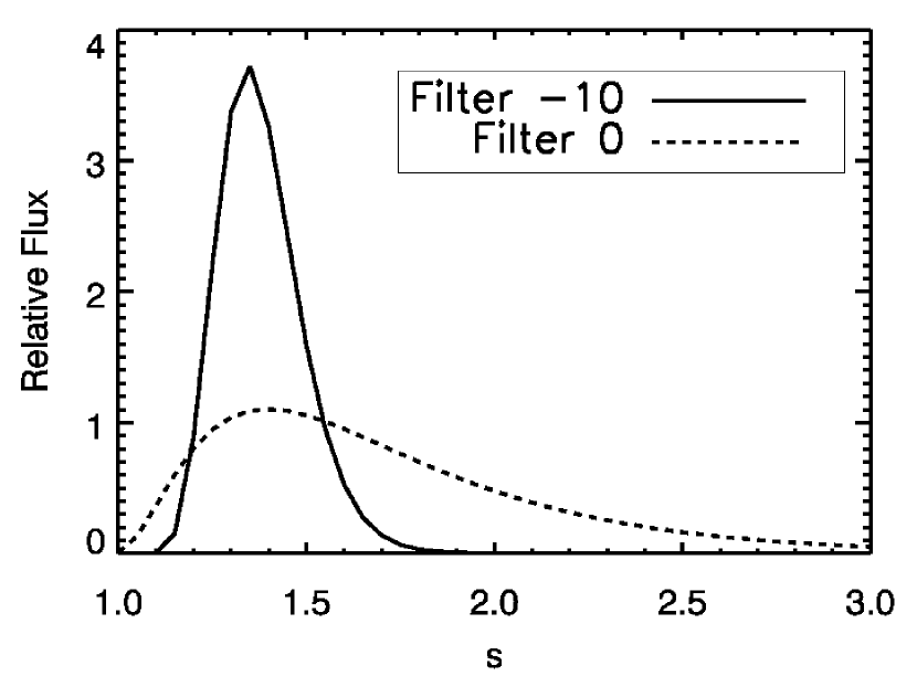
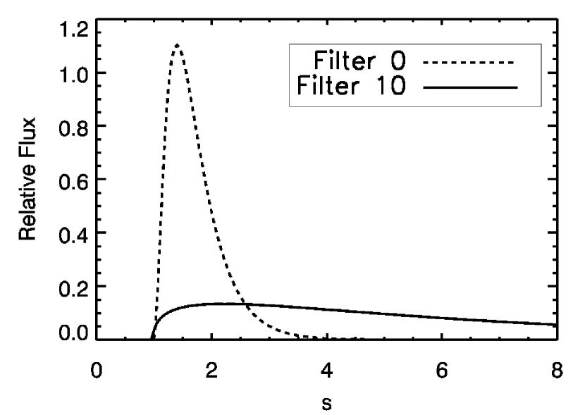
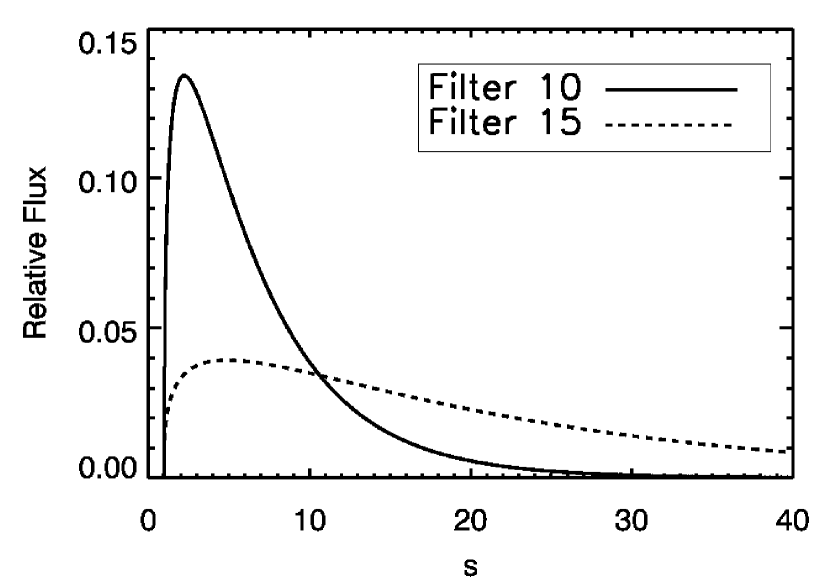
Figure 1: Radial surface brightness distributions ($2\pi sB_{i}(s)$) for an $r_{in}=0.2r_{E}$ Shakura-Sunyaev disk model in four filters, with central dimensionless wavelengths $x_{-10}=0.0271$, $x_{0}=0.2014$, $x_{10}=1.498$, and $x_{15}=4.086$. The vertical axis is normalized so that the integrated surface brightness equals unity.

Radial surface brightness profiles in four filters are shown in Figure 1.

The Shakura-Sunyaev disk model that we end up with depends on two parameters: $r_{in}$, the innermost radius of the disk, and $i$, the filter number. The temperature $T_{0}$ only determines the relation between $\lambda$ and $x$.

2.5 Other Models

Our Shakura-Sunyaev disk model is similar to the thin accretion disk models used by Agol & Krolik (1999) and Jaroszyński et al. (1992). Those models are more complicated, however, as they include rotating black holes, tilted disks, and relativistic effects. Microlensing simulations with nonthermal models have also been considered (Rauch & Blandford, 1991), but we do not include such models in this study.

3 MAGNIFICATION MAPS

The effect of microlenses on the total macroimage flux may be represented by a magnification map in the source plane, where the value at each point of the map is equal to the magnification of the source at that point, relative to the average macroimage magnification (Kayser et al., 1986; Paczyński, 1986; Wambsganss, 1990; Wambsganss et al., 1990b). The microlensing light curve of a small, point-like source can be found by tracing a path across the magnification map (e.g., Paczyński, 1986; Wambsganss et al., 1990b; Kochanek, 2004). For an extended source, we must first convolve the source profile with the magnification map to find the magnification due to microlensing at each location in the source plane (e.g., Wyithe et al., 2002).

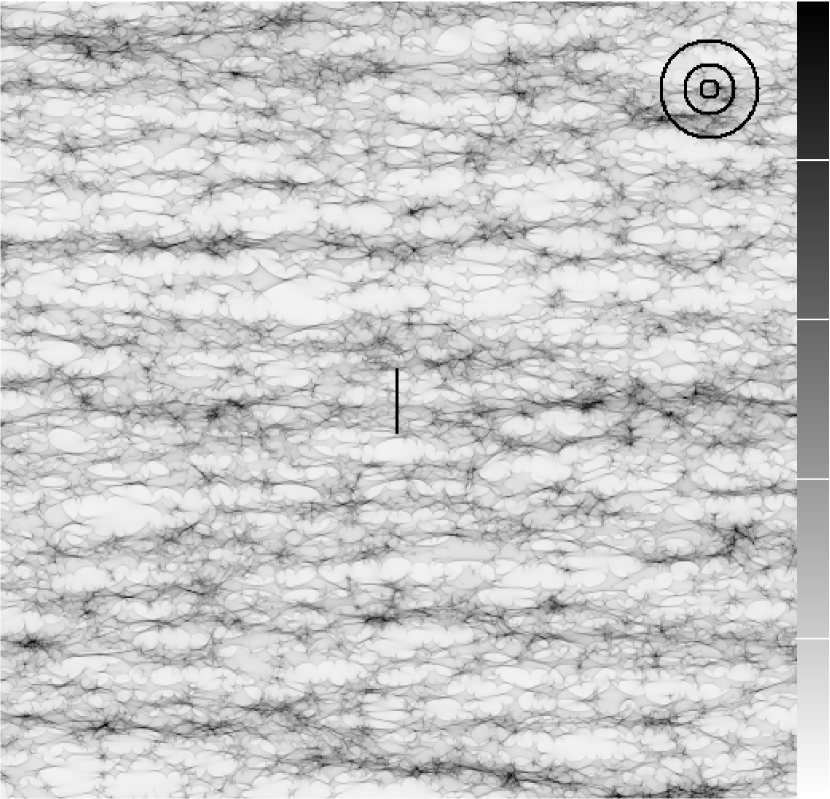
Figure 2: Magnification maps in the source plane for a positive parity image with $\kappa=\gamma=0.4$ (top) and a negative parity image with $\kappa=\gamma=0.6$ (bottom). The length of each side is 100 Einstein radii. The white lines on the greyscale bar correspond to magnifications that are 1, 2, 3, and 4 times the average macroimage magnification. Dark regions have greater magnification than light regions. The black circles have radii of 1, 3, and 6 Einstein radii for comparison with the Shakura-Sunyaev disk models. The black vertical line in the top map shows the path used for the light curves in Figure 4.

The maps were made using ray-shooting techniques that simulate sending rays from the observer through the lens to the source plane (Kayser et al., 1986; Schneider & Weiss, 1987; Wambsganss, 1990; Wambsganss et al., 1990a, b; Wambsganss, 1999). The maps are 2000 by 2000 pixel arrays with sides of length 100 Einstein radii. We examined two cases typical of the images that might be formed by a galaxy lensing a quasar: a positive parity image (minimum of the time-delay function) with convergence $\kappa=0.4$ (all in compact objects), shear $\gamma=0.4$, and theoretical average magnification $\mu=5$; and a negative parity image (saddle point) with $\kappa=0.6$ (again, all in compact objects), $\gamma=0.6$, and $\mu=-5$. Magnification maps for each case are shown in Figure 2. The positive parity simulation included 37,469 lenses, and the negative parity simulation included 56,224 lenses.

For each disk model we wished to study, we used the relevant equation from Section 2 to create a 2000 by 2000 pixel array for the disk brightness profile, $A$. Let us call the original magnification map $M$. By the convolution theorem, we can convolve $M$ and $A$ by multiplying their two-dimensional Fourier transforms and then taking the inverse Fourier transform of the product. This produces a new 2000 by 2000 pixel magnification map,

$$C={\rm fft}^{-1}\left[{\rm fft}(M){\rm fft}(A)\right],$$ (12)

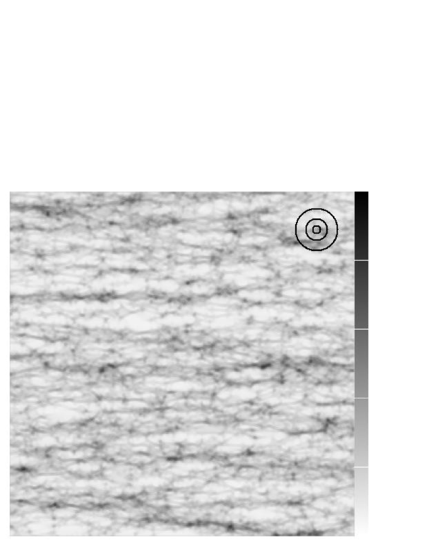
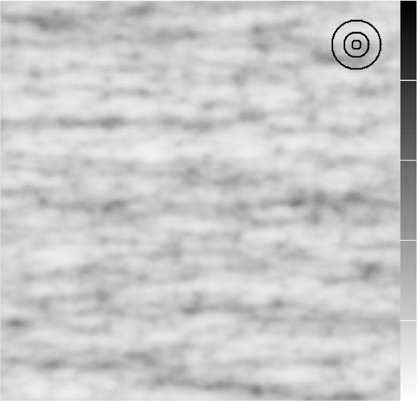
Figure 3: Examples of magnification maps from convolving Shakura-Sunyaev disk profiles with the original positive parity pattern in Figure 2. The innermost radius of each disk is $r_{in}=0.2r_{E}$. For the top map, the filter is $i=0$ with central wavelength $x_{0}$, the wavelength of the peak of the blackbody distribution at the maximum temperature $T_{0}$; the disk surface brightness peaks around $r=1.4r_{in}$ at this wavelength. For the bottom map the filter is $i=10$ with central wavelength $x_{10}=7.44x_{0}$, and the peak surface brightness is approximately at $r=2.2r_{in}$. The scale and the reference circles are the same as in Figure 2.

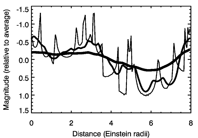
Figure 4: Sample light curves from the positive parity magnification map in Figure 2 and both maps in Figure 3 ($\kappa=\gamma=0.4$). The source travels on a vertical path of length 4 Einstein radii in the center of each map (the black line in the first panel of Figure 2). The thin curve is from the unconvolved positive parity map, the medium curve is from the convolution with the disk viewed in the filter associated with the peak surface brightness at the maximum temperature $T_{0}$ ($i=0$), and the thick curve is from the convolution in the filter that is a factor of 7.44 longer in wavelength ($i=10$).

where fft and fft^-1 stand for the fast Fourier transform and the inverse fast Fourier transform, respectively (e.g., Press et al., 1992). Figure 3 shows two examples of magnification maps from convolutions with Shakura-Sunyaev disk models. Sample light curves for paths through these maps are shown in Figure 4.

The longest wavelengths used in our simulations were chosen so that at least 95% of the total accretion disk intensity would lie within the 2000 by 2000 pixel area of the magnification map. At longer wavelengths, the cooler temperatures of the disk at large radii make the outer regions of the disk more important than in the shorter-wavelength filters. If we use too long a wavelength, a large fraction of the disk intensity spills out of the area of our simulation, making the results inaccurate. The wavelength at which this occurs varies with $r_{in}$. Although the cutoff is 95%, for the majority of filters used the fraction of light included in the 2000 by 2000 pixel area is above 99%.

At the short-wavelength end, the cutoff was more arbitrary since the disk profiles and their magnification histograms do not vary much with wavelength beyond a certain point that depends on the value of $r_{in}$. We chose to use wavelengths short enough to probe values of the half-light radius (see Section 4.2) close to the inner radius $r_{in}$ (within one Einstein radius).

4 MAGNIFICATION HISTOGRAMS

4.1 Histograms of Convolutions with Shakura-Sunyaev Disks

The values in a magnification map are ratios of the macroimage’s flux at Earth when the source is at a particular point in the map, $F({\emph{\bf r}})$, to the average macroimage flux, $\bar{F}=\mu F_{s}$, where $F_{s}$ is the flux of the unlensed source at Earth. We convert these ratios to magnitude differences,

$$\Delta m({\emph{\bf r}})=-2.5\log_{10}\left(\frac{F({\emph{\bf r}})}{\bar{F}}\right)$$ (13)

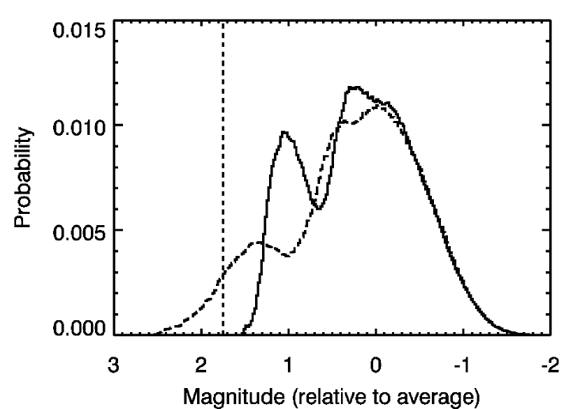
Figure 5: Magnification histograms for the unconvolved magnification maps in Figure 2. The solid histogram is from the positive parity image and the dotted one is from the negative parity image. The bin width for each histogram is 0.02 mag. The dispersions of the solid and dotted histograms are 0.67 and 0.81, respectively. The dashed vertical line shows the cutoff at unit magnification for the positive parity image.

and plot a histogram of $\Delta m$ for the convolution with each disk model, as in Wambsganss (1992). The number of pixels that fall into each bin of $\Delta m$ is represented as a probability for the macroimage to have a certain magnitude shift by dividing the number of pixels in the bin by the total number of pixels. Histograms of the original magnification maps are shown in Figure 5. Both histograms have two main peaks, typical for images with $|\mu|=5$ (Schechter & Wambsganss, 2002). A minimum (positive parity) must have at least unit magnification, so the positive parity histogram is cut off at the low-magnification end. At lower magnification, the negative parity histogram has a tail that extends down to $\Delta m\sim 2-3$ mag. The left peak of each histogram (around $\Delta m=1-1.5$ mag) is associated with the case of no extra microimage minima, while the right peak around $\Delta m=0$ mag is associated with the case of one extra microimage pair (Rauch et al., 1992).

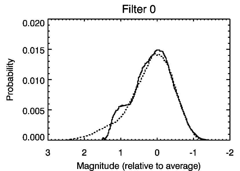
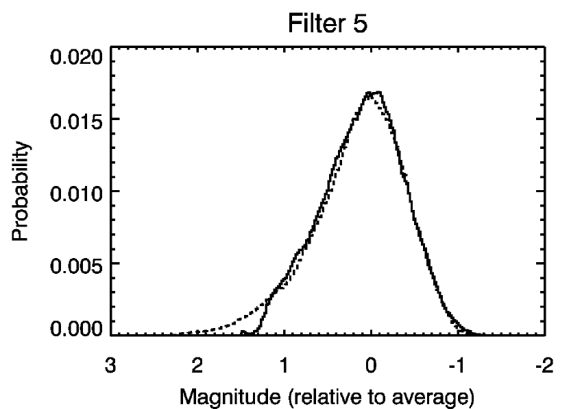
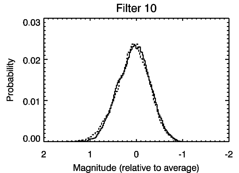
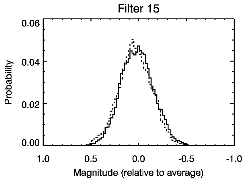
Figure 6: Histograms of magnitudes (relative to the magnitude that corresponds to the average macroimage flux at Earth) for convolutions of Shakura-Sunyaev disk profiles with $r_{in}=0.2r_{E}$ in various filters with the positive parity $\kappa=\gamma=0.4$ magnification map (solid curves) and the negative parity $\kappa=\gamma=0.6$ magnification map (dashed curves). The half-light radii of the disks used as sources are $0.28r_{E}$, $0.41r_{E}$, $1.00r_{E}$, and $3.32r_{E}$, respectively. The histograms at shorter wavelengths than that of the filter associated with the peak surface brightness at the maximum temperature $T_{0}$ (upper left) are all very similar, so they are not shown here.

We constructed magnification maps for convolutions with Shakura-Sunyaev disks in several filters with $r_{in}=0.2r_{E}$, $0.5r_{E}$, $r_{E}$, and $3r_{E}$, where $r_{E}$ is the microlens Einstein radius. Histograms from some of these maps are shown in Figures 6 and 7. For long wavelengths or large $r_{in}$, the histograms are sharply peaked at the average macroimage magnification, and there is little difference between the positive and negative parity cases. These characteristics reflect the loss of detail in the magnification maps for convolutions with disks that have large effective sizes. As we discuss in Sections 4.3 and 5, these disks are probably unrealistically large relative to the microlens Einstein radius, so the results that follow are valid in the limit of very small microlenses or very large disks. However, some of the results we find should be true for more general lens systems.

4.2 Histogram Statistics

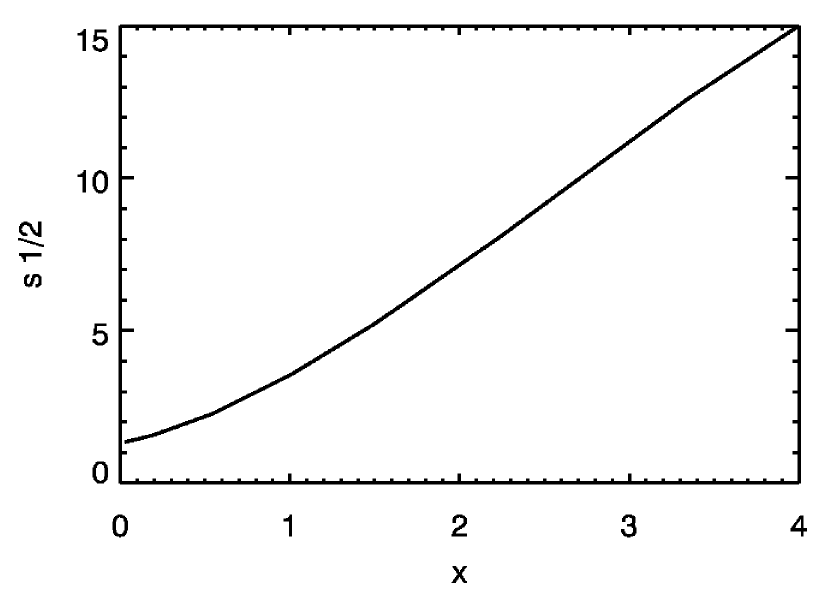
Figure 8: Dimensionless half-light radius ($s_{1/2}=r_{1/2}/r_{in}$) versus dimensionless wavelength, $x$, for the Shakura-Sunyaev models.

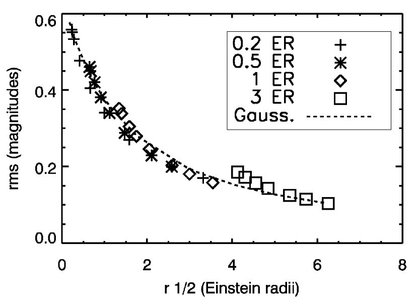
Figure 9: Dispersion (rms) and skewness of convolutions of the $\kappa=\gamma=0.4$ magnification map with various Shakura-Sunyaev disk profiles. Different plot symbols are used for different values of $r_{in}$ (given in Einstein radii). Dashed curves for the Gaussian disk models are shown for comparison. Note that negative skewness is associated with a tail toward dimmer (positive) magnitudes.

Since the surface brightness from disks in different filters falls off with radius at different rates, we can use the half-light radius, $r_{1/2}$, as a proxy for wavelength (see Figure 8). For each magnification histogram, we calculated the dispersion (root mean square or rms) and skewness of the data and plotted these statistics against $r_{1/2}/r_{E}$. The results are shown in Figures 9 and 10.

For all disk sizes, the dispersion decreases with $r_{1/2}/r_{E}$. This shows that the effect of microlensing is diminished at longer wavelengths and for larger disks. These trends are expected since the source must be smaller than the microlens Einstein radius for microlensing to play a significant role.

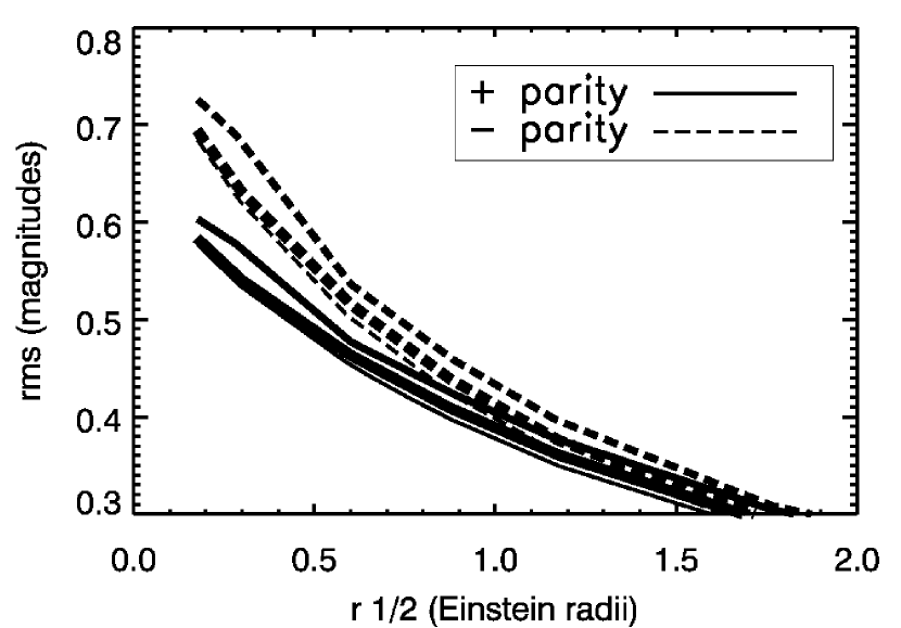
Figure 11: Dispersion (rms) of histograms from convolutions of both positive ($\kappa=\gamma=0.4$, solid curves) and negative ($\kappa=\gamma=0.6$, dashed curves) parity magnification maps with Gaussian disks (thin curves), uniform disks (medium), and cones (thick). For values of $r_{1/2}$ greater than about 2 Einstein radii, the six curves shown here are nearly indistinguishable.

Using the same methods described in Section 4.1, we produced magnification histograms from convolutions with Gaussian disks, uniform disks, and cones. These histograms all have very similar dispersion and skewness as a function of $r_{1/2}$; the dispersion results are shown in Figure 11. From Figures 9 and 10 we see that, for a given value of $r_{1/2}$, there is little practical difference between the dispersions of histograms produced with the Gaussian disks and those produced with the Shakura-Sunyaev accretion disk models. This suggests that, to a good approximation, the microlensing fluctuations only depend on $r_{1/2}$, and the disk may be modeled with any reasonable surface brightness profile. We examine this claim more quantitatively in the last paragraph of this section.

In the third moment of the histograms, the skewness, we begin to see some greater differences between the Shakura-Sunyaev models and the Gaussian models (lower panels in Figures 9 and 10). However, since skewness is much more difficult to measure with observations than dispersion, these differences may well be unimportant for most applications.

We also used chi-square tests to compare histograms from convolutions with disks that have different shapes and different sizes. Histograms associated with uniform disks require about 10,000 independent observations to distinguish them with 95% confidence from histograms associated with Shakura-Sunyaev disks of the same size; the comparisons between the Gaussian disks or cones and the Shakura-Sunyaev disks need an even greater number of observations, around 40,000. In contrast, the size comparisons tend to require far fewer observations. After examining many sizes of Gaussian disk models and comparing the histograms of their convolutions, we found that to tell apart histograms associated with Gaussian disks that differ in size by $0.25r_{E}$ (a quarter of an Einstein radius), it requires 2000 to 4000 independent observations to reach 95% confidence. If we make the difference in size much smaller, the number of observations can be as large as for the shape comparisons (for example, a $0.05r_{E}$ size difference in Gaussian disks calls for around 40,000 observations for 95% confidence), but in this case the disks with different sizes are intrinsically much more similar than the disks with different shapes, so it is no surprise that the histograms that arise from convolutions with the disks with slightly different sizes are also very similar to each other.

4.3 Physical Values for Typical Quasars

The results of the previous sections for Shakura-Sunyaev disks are given in terms of a dimensionless wavelength, $x$, and radius, $r_{in}$. To understand how these results might apply to actual microlensed quasars, we must convert this wavelength and radius into physical quantities.

For a “typical” quasar, we will assume that there is a central black hole with mass $M=10^{8}$ M_⊙ and that the bolometric luminosity of the quasar is $L=10^{46}$ erg s^-1 (e.g., Frank et al., 1992). From Yu & Tremaine (2002), we will take the efficiency for the quasar to be $\eta=0.2$, which gives an accretion rate $\dot{M}=5\times 10^{26}$ g s^-1. Doing a simple Newtonian calculation with these numbers yields an innermost radius $r_{in}=2.5M=3\times 10^{14}$ cm. These values of $\dot{M}$ and $r_{in}$ are close to the typical quasar values given in Frank et al. (1992). Using the formulas for a Kerr black hole from Bardeen et al. (1972), we can quantify the error due to the Newtonian calculation. An innermost stable circular orbit at $r_{in}=2.5M$ corresponds to a black hole spin of $a=0.879$. This gives a binding energy per mass of 0.146, which is reasonably close to the assumed value of $\eta=0.2$ at the level of accuracy at which we are working.

By comparing the constant factor in the temperature-radius relation found in Frank et al. (1992) to that in Equation (3), we find that the maximum disk temperature is

$$T_{0}=0.488\left(\frac{3GM\dot{M}}{8\pi\sigma r_{in}^{3}}\right)^{1/4},$$ (14)

where $G$ is Newton’s constant and $\sigma$ is the Stefan-Boltzmann constant. Using the values listed above for $M$, $\dot{M}$, and $r_{in}$, the maximum temperature is $T_{0}=7.4\times 10^{4}$ K.

Using these results, we can compare the filters of the Shakura-Sunyaev disk model to a real filter. For example, the Sloan $r^{\prime}$ filter covers a range of wavelengths from about $5560~{}{\rm\AA}$ to $6950~{}{\rm\AA}$ (Fukugita et al., 1996). Taking the maximum temperature of the accretion disk to be $T_{0}=7.4\times 10^{4}$ K and assuming that the source is at redshift $z_{S}=2.0$, the Sloan $r^{\prime}$ filter corresponds to a range of dimensionless wavelengths $0.95<x<1.18$. This is closest to the filter we label $i=8$, which has a range $0.90<x<1.10$. The filter $i=8$ falls in the middle of the range of filters used in this study, so the artificial filters we used are close approximations to some real filters.

Next, we can compare the radii of the Shakura-Sunyaev disk models to physical radii. As mentioned earlier, our typical quasar has an innermost radius $r_{in}=3\times 10^{14}$ cm. For a lens at redshift $z_{L}=0.5$ and a source at redshift $z_{S}=2.0$, the Einstein radius of a 1-M_⊙ microlens is $r_{E}\approx 5.7\times 10^{17}$ cm (Wambsganss, 1992). With these values, then, $r_{in}=0.0005r_{E}$. This is considerably smaller than the $r_{in}$ to $r_{E}$ ratios examined in this study. Of course, the exact ratio depends on the various masses and other parameters that we assume, but to have $r_{in}\sim r_{E}$ requires either very massive black holes or very small microlensing objects. Therefore, Shakura-Sunyaev disks with physically realistic sizes are likely to be smaller than the disks we modeled by at least an order of magnitude. However, the smallest disk we considered ($r_{in}=0.2r_{E}$) produces magnification histograms that are at least qualitatively similar, at short wavelengths, to the histograms for a point source (Figure 5). As we reduce the disk size from $r_{1/2}=0.28r_{E}$ (the $r_{in}=0.2r_{E}$ disk in filter $i=0$) to $r_{1/2}=0$, the magnification histogram changes from that in the upper left panel of Figure 6 (dispersion 0.53 for positive parity, 0.62 for negative parity) to that in Figure 5 (dispersion 0.63 for positive parity, 0.77 for negative parity). A disk with a realistic half-light radius would have a magnification histogram that is practically identical to the corresponding histogram in Figure 5.

This result suggests that, for “typical” Shakura-Sunyaev disks, not only the shape but also the size can be ignored in most cases, so the source behaves like a point source to a good approximation. Therefore, we would not expect to see significant chromatic effects for typical Shakura-Sunyaev disks. An important exception is high-magnification events that occur when the source crosses a caustic (e.g., Wyithe et al., 2000a; Yonehara, 2001; Shalyapin et al., 2002; Wyithe et al., 2002; Schechter et al., 2003), but away from caustics the results found here apply.

5 CONCLUSIONS

We have produced several magnification histograms by convolving quasar source brightness profiles with a variety of shapes and sizes with both positive and negative parity image magnification patterns. These histograms can be thought of as distributions of the probability to observe the quasar macroimage with a certain magnification. We compared histograms associated with accretion disks of different shapes and different sizes by computing moments of the histograms (dispersion and skewness), and by computing chi-square values for pairs of histograms.

By plotting dispersion and skewness against half-light radius (Figures 9 and 10), we discovered that for any particular disk model there is a clear dependence of dispersion and skewness on the half-light radius, but if we compare disk models with different shapes but the same half-light radius, the dispersion and skewness of the associated histograms are only slightly dependent on the shape of the model. This suggests that size differences have a more significant effect on microlensing fluctuations than shape differences do, at least for circular sources.

The chi-square tests confirm this result. When comparing magnification histograms, the number of observations needed to distinguish sources with differently-shaped brightness profiles but the same size is significantly higher than the amount needed to tell the difference between sources with different sizes but the same shape of the brightness distribution.

This is strong evidence that the dependence of microlensing variability on source shape is far weaker than the dependence on source size. We can model the accretion disk by any circular brightness profile we like—Gaussian disk, uniform disk, or any other well-behaved disk model—and our model will produce the correct results, as long as it is the correct size.

Since the physically-motivated disk model we studied was larger than what one would expect to observe, further studies of smaller, more typical Shakura-Sunyaev disks could help clarify the validity of these conclusions. However, our results are valid in the limits of extremely small microlenses or large black holes, and we can conclude in general that if any physical properties of a disk have an effect on the microlensing of quasars away from caustics, it is the half-light radius of the source and not the shape of its brightness profile.

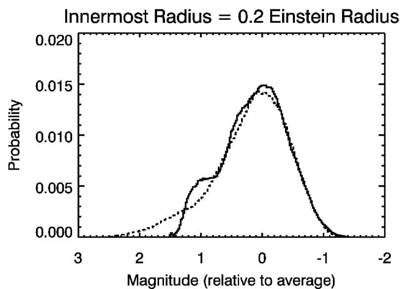
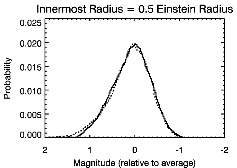
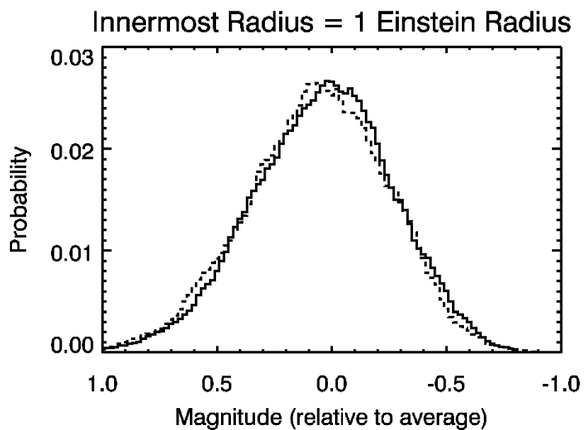
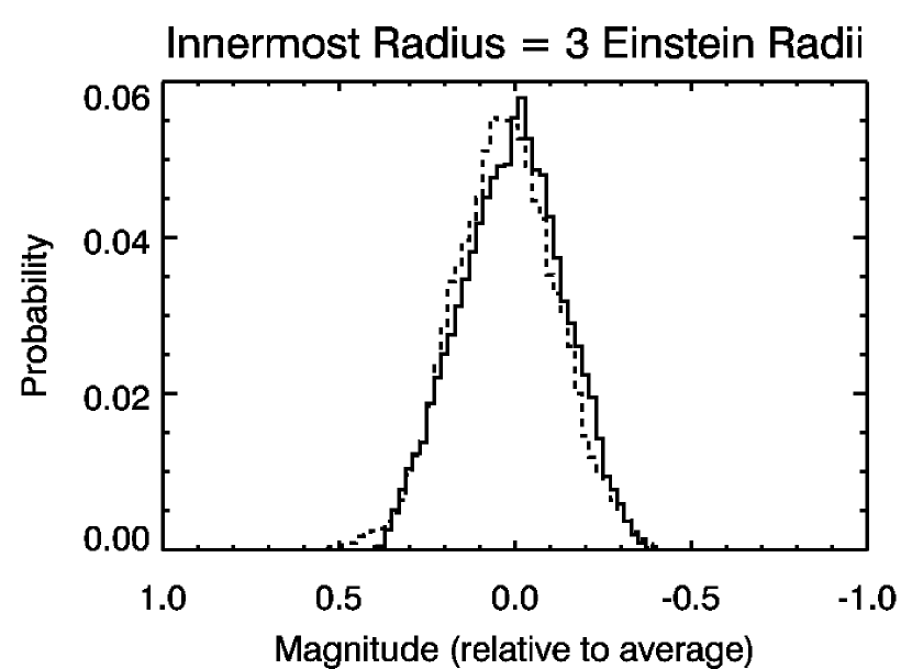
Figure 7: Histograms of magnitudes relative to the average for convolutions of Shakura-Sunyaev disk profiles of various sizes in the filter associated with the peak surface brightness at the maximum temperature $T_{0}$ ($i=0$) with the positive parity $\kappa=\gamma=0.4$ magnification map (solid curves) and the negative parity $\kappa=\gamma=0.6$ magnification map (dashed curves). The half-light radii of the disks used as sources are $0.28r_{E}$, $0.77r_{E}$, $1.58r_{E}$, and $4.84r_{E}$, respectively.

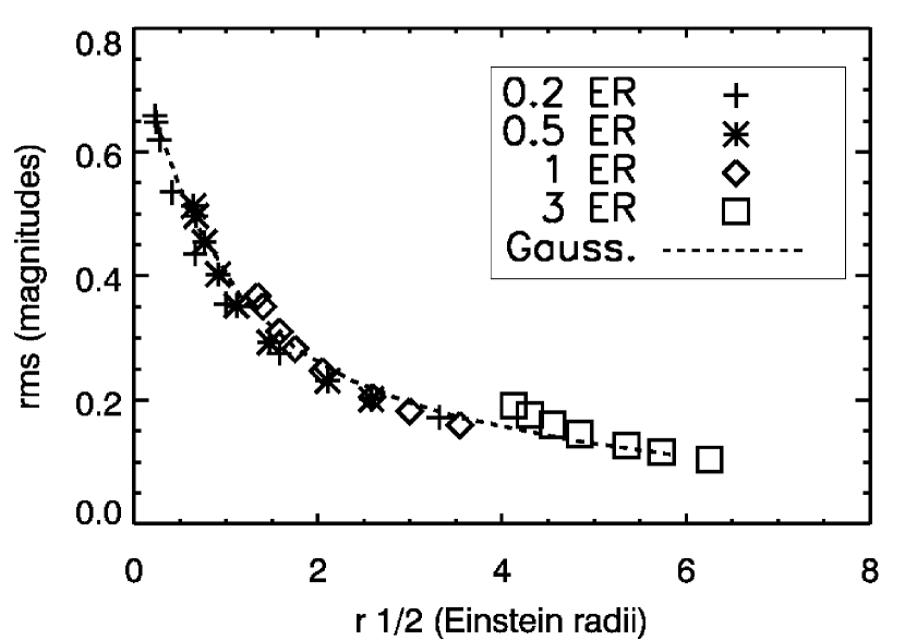
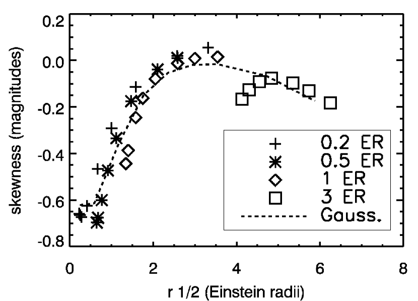
Figure 10: Same as Figure 9, here for the negative parity case $\kappa=\gamma=0.6$.

References

- Agol & Krolik (1999) Agol, E., & Krolik, J. 1999, ApJ, 524, 49
- Bardeen et al. (1972) Bardeen, J. M., Press, W. H., & Teukolsky, S. A. 1972, ApJ, 178, 347
- Burud et al. (2002) Burud, I., et al. 2002, A&A, 383, 71
- Chartas et al. (2004) Chartas, G., Eracleous, M., Agol, E., & Gallagher, S. C. 2004, ApJ, 606, 78
- Chiba (2002) Chiba, M. 2002, ApJ, 565, 17
- Courbin et al. (2002) Courbin, F., Saha, P., & Schechter, P. 2002, in Gravitational Lensing: An Astrophysical Tool, ed. F. Courbin & D. Minniti (Berlin: Springer), 1
- Dalal & Kochanek (2002) Dalal, N., & Kochanek, C. S. 2002, ApJ, 572, 25
- Dobler & Keeton (2005) Dobler, G., & Keeton, C. R. 2005, preprint (astro-ph/0502436)
- Frank et al. (1992) Frank, J., King, A., & Raine, D. 1992, Accretion Power in Astrophysics (2nd ed.; Cambridge: Cambridge University Press)
- Fukugita et al. (1996) Fukugita, M., Ichikawa, T., Gunn, J. E., Doi, M., Shimasaku, K., & Schneider, D. P. 1996, AJ, 111, 1748
- Gould & Miralda-Escudé (1997) Gould, A., & Miralda-Escudé, J. 1997, ApJ, 483, L13
- Grieger et al. (1988) Grieger, B., Kayser, R., & Refsdal, S. 1988, A&A, 194, 54
- Irwin et al. (1989) Irwin, M. J., Webster, R. L., Hewett, P. C., Corrigan, R. T., & Jedrzejewski, R. I . 1989, AJ, 98, 1989
- Jaroszyński et al. (1992) Jaroszyński, M., Wambsganss, J., & Paczyński, B. 1992, ApJ, 396, L65
- Kayser et al. (1986) Kayser, R., Refsdal, S., & Stabell, R. 1986, A&A, 166, 36
- Kochanek (2004) Kochanek, C. S. 2004, ApJ, 605, 58
- Lewis & Ibata (1998) Lewis, G. F., & Ibata, R. A. 1998, ApJ, 501, 478
- Metcalf & Madau (2001) Metcalf, R. B., & Madau, P. 2001, ApJ, 563, 9
- Metcalf et al. (2003) Metcalf, R. B., Moustakas, L. A., Bunker, A. J., & Parry, I. R. 2004, ApJ, 607, 43
- Mineshige & Yonehara (1999) Mineshige, S., & Yonehara, A. 1999, PASJ, 51, 497
- Moustakas & Metcalf (2003) Moustakas, L. A., & Metcalf, R. B. 2003, MNRAS, 339, 607
- Paczyński (1986) Paczyński, B. 1986, ApJ, 301, 503
- Press et al. (1992) Press, W. H., Teukolsky, S. A., Vetterling, W. T., & Flannery, B. P. 1992, Numerical Recipes in C (2nd ed.; Cambridge: Cambridge University Press)
- Rauch & Blandford (1991) Rauch, K. P., & Blandford, R. D. 1991, ApJ, 381, L39
- Rauch et al. (1992) Rauch, K. P., Mao, S., Wambsganss, J., & Paczyński, B. 1992, ApJ, 386, 30
- Refsdal & Stabell (1997) Refsdal, S., & Stabell, R. 1997, A&A, 325, 877
- Schechter et al. (1998) Schechter, P. L., Gregg, M. D., Becker, R. H., Helfand, D. J., & White, R. L. 1998, AJ, 115, 1371
- Schechter & Wambsganss (2002) Schechter, P. L., & Wambsganss, J. 2002, ApJ, 580, 685
- Schechter et al. (2003) Schechter, P. L., et al. 2003, ApJ, 584, 657
- Schneider & Weiss (1987) Schneider, P., & Weiss, A. 1987, A&A, 171, 49
- Shakura & Sunyaev (1973) Shakura, N. I., & Sunyaev, R. A. 1973, A&A, 24, 337
- Shalyapin et al. (2002) Shalyapin, V. N., Goicoechea, L. J., Alcalde, D., Mediavilla, E., Muñoz, J. A., & Gil-Merino, R. 2002, ApJ, 579, 127
- Takahashi et al. (2001) Takahashi, R., Yonehara, A., & Mineshige, S. 2001, PASJ, 53, 387
- Treyer & Wambsganss (2004) Treyer, M., & Wambsganss, J. 2004, A&A, 416, 19
- Vakulik et al. (2003) Vakulik, V. G., et al. 2004, A&A, 420, 447
- Wambsganss (1990) Wambsganss, J. 1990, Ph.D. thesis, Ludwig-Maximilians-Universität, München, available as MPA550, Max-Planck-Institut für Astrophysik
- Wambsganss (1992) Wambsganss, J. 1992, ApJ, 386, 19
- Wambsganss (1999) Wambsganss, J. 1999, J. Comput. Appl. Math., 109, 353
- Wambsganss & Paczyński (1991) Wambsganss, J., & Paczyński, B. 1991, AJ, 102, 864
- Wambsganss et al. (1990a) Wambsganss, J., Paczyński, B., & Katz, N. 1990a, ApJ, 352, 407
- Wambsganss et al. (1990b) Wambsganss, J., Schneider, P., & Paczyński, B. 1990b, ApJ, 358, L33
- Wisotzki et al. (2003) Wisotzki, L., Becker, T., Christensen, L., Helms, A., Jahnke, K., Kelz, A., Roth, M. M., & Sanchez, S. F. 2003, A&A, 408, 455
- Wisotzki et al. (1993) Wisotzki, L., Koehler, T., Kayser, R., & Reimers, D. 1993, A&A, 278, L15
- Witt et al. (1995) Witt, H. J., Mao, S., & Schechter, P. L. 1995, ApJ, 443, 18
- Woźniak et al. (2000a) Woźniak, P. R., Alard, C., Udalski, A., Szymański, M., Kubiak, M., Pietrzyński, G., Zebruń, K. 2000a, ApJ, 529, 88
- Woźniak et al. (2000b) Woźniak, P. R., Udalski, A., Szymański, M., Kubiak, M., Pietrzyński, G., Soszyński, I., & Zebruń, K. 2000b, ApJ, 540, L65
- Wyithe et al. (2002) Wyithe, J. S. B., Agol, E., & Fluke, C. J. 2002, MNRAS, 331, 1041
- Wyithe et al. (2000a) Wyithe, J. S. B., Webster, R. L., & Turner, E. L. 2000a, MNRAS, 318, 762
- Wyithe et al. (2000b) Wyithe, J. S. B., Webster, R. L., Turner, E. L., & Agol, E. 2000b, MNRAS, 318, 1105
- Yonehara (2001) Yonehara, A. 2001, ApJ, 548, L127
- Yonehara et al. (1999) Yonehara, A., Mineshige, S., Fukue, J., Umemura, M., & Turner, E. L. 1999, A&A, 343, 41
- Yonehara et al. (1998) Yonehara, A., Mineshige, S., Manmoto, T., Fukue, J., Umemura, M., & Turner, E. L. 1998, ApJ, 501, L41
- Yu & Tremaine (2002) Yu, Q., & Tremaine, S. 2002, MNRAS, 335, 965