Dust Dynamics in Compressible MHD Turbulence

Abstract

We calculate the relative grain-grain motions arising from interstellar magnetohydrodynamic (MHD) turbulence. The MHD turbulence includes both fluid motions and magnetic fluctuations. While the fluid motions accelerate grains through hydro-drag, the electromagnetic fluctuations accelerate grains through resonant interactions. We consider both incompressive (Alfvén) and compressive (fast and slow) MHD modes and use descriptions of MHD turbulence obtained in Cho & Lazarian (2002). Calculations of grain relative motion are made for realistic grain charging and interstellar turbulence that is consistent with the velocity dispersions observed in diffuse gas, including cutoff of the turbulence from various damping processes. We show that fast modes dominate grain acceleration, and can drive grains to supersonic velocities. Grains are also scattered by gyroresonance interactions, but the scattering is less important than acceleration for grains moving with sub-Alfvénic velocities. Since the grains are preferentially accelerated with large pitch angles, the supersonic grains will be aligned with long axes perpendicular to the magnetic field. We compare grain velocities arising from MHD turbulence with those arising from photoelectric emission, radiation pressure and H₂ thrust. We show that for typical interstellar conditions turbulence should prevent these mechanisms from segregating small and large grains. Finally, gyroresonant acceleration is bound to preaccelerate grains that are further accelerated in shocks. Grain-grain collisions in the shock may then contribute to the overabundance of refractory elements in the composition of galactic cosmic rays.

1 Introduction

Dust is an important constituent of the interstellar medium (ISM). It interferes with observations in the optical range, but provides an insight to star-formation activity through far-infrared radiation. It also enables molecular hydrogen formation and traces the magnetic field via emission and extinction polarization (see reviews by Hildebrand et al. 2000, Lazarian 2000, 2002). The basic properties of dust (extinction, polarization, etc.) strongly depend on its size distribution. The latter evolves as the result of grain collisions, whose frequency and consequences depend on grain relative velocities (see discussions in Draine 1985, Lazarian & Yan 2002ab).

Grain-grain collisions can have various outcomes, e.g., coagulation, cratering, shattering, and vaporization. For collisions with $\delta v\leq 10^{-3}$km/s, grains are likely to stick or coagulate, as the potential energy due to surface forces exceeds the initial center of mass kinetic energy. Coagulation is considered the mechanism to produce large grains in dark clouds and accretion disks. Collisions with $\delta v\geq 20$km/s have sufficient energy to vaporize at least the smaller of the colliding grains (Draine 1985). It is likely that some features of the grain distribution, e.g., the cutoff at large size (e.g., Kim, Martin & Hendry 1994), are the result of fragmentation (Biermann & Harwit 1980). Even low-velocity grain collisions may have dramatic consequences by triggering grain mantle explosion (Greenberg & Yencha 1973, Schutte & Greenberg 1991).

Various processes can affect the velocities of dust grains. Radiation, ambipolar diffusion, and gravitational sedimentation all can bring about a dispersion in grain velocities. It is widely believed that, except in special circumstances (e.g., near a luminous young star, or in a shock wave), none of these processes can provide substantial random velocities so as to affect the interstellar grain population via collisions (Draine 1985), except for possibly enhancing the coagulation rate. Nevertheless, de Oliveira-Costa et al. (2002) speculated that starlight radiation can produce the segregation of different sized grains that was invoked to explain the imperfect correlation of the microwave and $100\mu$m signals of the foreground emission (Mukherjee et al. 2001). If true it has important implications for the CMB foreground studies. However, the efficiency of this segregation depends on grain random velocities, which we study in this paper.

The interstellar medium is magnetized and turbulent (see Arons & Max 1975, Scalo 1987, Lazarian 1999). Although turbulence has been invoked by a number of authors (see Kusaka et al. 1970, Völk et al. 1980, Draine 1985, Ossenkopf 1993, Weidenschilling & Ruzmaikina 1994) to provide substantial grain relative motions, the turbulence they discussed was not magnetized. Dust grains are charged, and their interactions with magnetized turbulence are very different from the hydrodynamic case. Lazarian & Yan (2002a, henceforth LY02 and 2002b) applied the theory of Alfvénic turbulence (Goldreich & Sridhar 1995, henceforth GS95, see Cho, Lazarian & Vishniac 2002a for a review) to grain acceleration and considered the motions that emerge due to incomplete coupling of grains and gas. Unlike the pure hydrodynamic case discussed by earlier authors, LY02 took into account that the motions of grains are restricted by magnetic fields in the direction perpendicular to the field lines, and also took into account the anisotropy of Alfvénic turbulence.

While Alfvénic turbulence is the turbulence in an incompressible fluid, the ISM is highly compressible. Compressible MHD turbulence has been studied recently (see review by Cho & Lazarian 2003a and references therein). In Yan & Lazarian (2003, henceforth YL03) we identified a new mechanism of grain acceleration– gyroresonance –that is based on the direct interaction of charged grains with MHD turbulence. YL03 provided a test calculation of grain acceleration in compressible MHD turbulence, both by hydro-drag and by gyroresonance (see also review by Lazarian & Yan 2003).

In what follows, we describe grain acceleration by MHD turbulence in different phases of the ISM. Solving the Fokker-Planck equation including simultaneously the hydro-drag and gyroresonance would be a formidable task that we do not attempt here. Instead, we try to simplify the problem by separating these two processes. For the random fluid drag, we use a simple scaling argument similar to the approach in Draine (1985) and LY02. While dealing with gyroresonance, we follow the approach adopted in YL03, i.e., we do not include the motion of ambient gas and assume that turbulence provides nothing but electromagnetic fluctuations. These approximations should yield correct answers when one of the mechanisms is dominant. When the accelerations arising from the two mechanisms are comparable the situation is more complicated, as the gaseous friction that we use for gyroresonance calculations will be, in general, affected by fluid motions. We do not develop explicit theory for this case. But taking into account that it is the motions at the decoupling scale that accelerate grains via hydro-drag, we think it is reasonable to estimate the velocity gains from the simultaneous action of hydro-drag and gyroresonance by adding them in quadrature.

To describe the turbulence we use the statistics of Alfvénic modes obtained in Cho, Lazarian & Vishniac (2002b, hereafter CLV02) and compressive modes obtained in Cho & Lazarian (2002, hereafter CL02, 2003bc). We apply our results to different phases of ISM, including the cold neutral medium (CNM), warm neutral medium (WNM), warm ionized medium (WIM), molecular cloud (MC) and dark cloud (DC) conditions, to estimate the implications for coagulation, shattering and segregation of grains.

In what follows, we introduce the statistical description of MHD turbulence and damping processes ($\S 2$), describe motions arising from hydro-drag ($\S 3$) and gyroresonance ($\S 4$), apply our results to various ISM phases ($\S 5$), discuss astrophysical implications of our results ($\S 6$), and provide the summary in $\S 7$.

2 MHD cascade and its damping

MHD perturbations can be decomposed into Alfvénic, slow and fast modes (see Alfvén & Fälthmmar 1963). Alfvénic turbulence is considered by many authors as the default model of interstellar magnetic turbulence. This is partially motivated by the fact that unlike compressive modes, the Alfvénic modes are essentially free of damping in a fully ionized medium (see Ginzburg 1961, Kulsrud & Pearce 1969). Important questions arise. Can the MHD perturbations that characterize turbulence be separated into distinct modes? Can the linear modes be used for this purpose? The separation into Alfvén and pseudo-Alfvén modes is the cornerstone of the Goldreich-Sridhar (1995, henceforth GS95) model of turbulence. This model and the legitimacy of the separation were tested successfully with numerical simulations (Cho & Vishniac 2000; Maron & Goldreich 2001; CLV02). Separation of MHD perturbations in compressible media into fast, slow and Alfvén modes is discussed in GS95, Lithwick & Goldreich 2001, and CL02. The actual decomposition of MHD turbulence into Alfvén, slow and fast modes was performed in CL02, and Cho & Lazarian (2003, henceforth CL03), who also quantified the intensity of the interaction between different modes (see below).

Unlike hydrodynamic turbulence, Alfvénic turbulence is anisotropic, with eddies elongated along the magnetic field (see Montgomery & Turner 1981, Shebalin, Matthaeus, & Montgomery 1983, Higdon 1984, Zank & Matthaeus 1992). This happens because it is easier to mix the magnetic field lines perpendicular to the direction of the magnetic field rather than to bend them. The GS95 model describes incompressible Alfvénic turbulence, which formally means that plasma $\beta\equiv P_{\rm gas}/P_{\rm mag}$, i.e., the ratio of gas pressure to magnetic pressure, is infinity. The turbulent velocity spectrum is easily obtained. Calculations in CLV02 prove that motions perpendicular to magnetic field lines are essentially hydrodynamic. As the result, energy transfer rate due to those motions is a constant $\dot{E_{k}}\sim v_{k}^{2}/\tau_{k}$, where $\tau_{k}$ is the energy eddy turnover time $\sim(v_{k}k_{\perp})^{-1}$, where $k_{\perp}$is the perpendicular component of the wave vector $\mathbf{k}$. The mixing motions couple to the wave-like motions parallel to magnetic field giving a critical balance condition, i.e., $k_{\bot}v_{k}\sim k_{\parallel}V_{A}$, where $k_{\parallel}$ is the parallel component of the wave vector $\mathbf{k}$, and $V_{A}$ is the Alfvén speed. From these arguments, the scale dependent anisotropy $k_{\parallel}\propto k_{\perp}$and a Kolmogorov-like spectrum for the perpendicular motions $v_{k}\propto k^{-1/3}$ can be obtained.

It was conjectured in Lithwick & Goldreich (2001) that the GS95 scaling should be approximately true for Alfvén and slow modes in moderately compressible plasma. For magnetically dominated (i.e., low $\beta$) plasma, CL02 showed that the coupling of Alfvénic and compressive modes is weak and that the Alfvénic and slow modes follow the GS95 spectrum. This is consistent with the analysis of HI velocity statistics (Lazarian & Pogosyan 2000, Stanimirovic & Lazarian 2001) as well as with electron density statistics (see Armstrong, Rickett & Spangler 1995). Calculations in Cho & Lazarian (2003, hereafter CL03) demonstrated that fast modes are marginally affected by Alfvén modes and follow acoustic cascade in both high and low $\beta$ media.

In what follows, we consider both Alfvén modes and compressive modes and use the description of those modes obtained in CL02 and CL03 to study dust acceleration by MHD turbulence.

The distribution of energy between compressive and incompressive modes depends, in general, on the driving of turbulence. CL02 and CL03 studied generation of compressive perturbations using random incompressive driving, obtaining an expression that relates the energy in fast $\sim\delta V_{f}^{2}$ and Alfvén $\sim\delta V_{A}^{2}$ modes,

$$(\delta V_{f}/\delta V_{A})^{2}\sim\delta V_{A}V_{A}/(V_{A}^{2}+C_{S}^{2}),$$

where $C_{S}$ is the sound speed. This relation testifies that at large scales incompressive driving can transfer an appreciable part of energy into fast modes. However, at smaller scales the drain of energy from Alfvén to fast modes is marginal. Therefore the cascades evolve without much cross talk. A more systematic study of different types of driving is required. In what follows we assume that equal amounts of energy are transfered into fast and Alfvén modes when driving is at large scales.

We show that while simple scaling relations are sufficient for obtaining the velocities arising from hydro-drag, much more sophisticated tools are necessary for calculating gyroresonance (see Yan & Lazarian 2002, henceforth YL02, YL03). The corresponding statistics of turbulence is presented in Appendix B.

At small scales the turbulence spectrum is truncated by damping. Various processes can damp the MHD motions. In partially ionized plasma, the ion-neutral collisions are the dominant damping process. In fully ionized plasma, there are basically two kinds of damping: collisional or collisionless damping (see Appendix A for details). Their relative importance depends on the mean free path $l=v_{th}\tau=6\times 10^{11}(T/8000K)^{2}\,{\rm cm}^{-2}/n$ in the ISM (Braginskii 1965). If the wavelength is larger than the mean free path, viscous damping dominates. If, on the other hand, the wavelength is smaller than mean free path, then the plasma is in the collisionless regime and collisionless damping is dominant.

To obtain the truncation scale, the damping time should be compared to the cascading time. As we mentioned earlier, the Alfvénic turbulence cascades over one eddy turn over time $(k_{\perp}v_{k})^{-1}\sim(k_{\parallel}V_{A})^{-1}$. The cascade of the fast modes is a bit slower:

$$\tau_{k}=\omega/k^{2}v_{k}^{2}=(k/L)^{-1/2}\times V_{f}/V^{2},$$ (1)

where $V_{f}$ is the phase velocity of fast waves, and $V$ is the turbulence velocity at the injection scale (CL02). If the damping is faster than the cascade, the turbulence is truncated. Otherwise, for the sake of simplicity, we ignore the damping and assume that the turbulence cascade is unaffected. According to CL02 the transfer of energy between Alfvén, slow and fast modes of MHD turbulence is suppressed. This allows us to consider different components of MHD cascade independently.

3 Grain Charge

The net electrical charge on a grain is the result of competition between collisions with electrons, which add negative charge, and photoelectric emission and collisions with ions, which remove negative charge. We assume the grains to be spheres consisting of either “astronomical silicate” or graphite, with absorption cross sections calculated as described by Weingartner & Draine (2001a; henceforth WD01a), and photoelectric yields (as a function of $Z$) estimated by Weingartner & Draine (2001b; henceforth WD01b).

The grain charge depends on the electron density $n_{e}$. While many previous studies have assumed cosmic ray ionization rates $\zeta\approx 1\times 10^{-17}{\rm s}^{-1}$ (e.g., Ruffle et al. 1998), recent observational determinations (Black & van Dishoeck 1991; Lepp 1992; McCall et al. 2003) suggest $\zeta\approx 1-10\times 10^{-16}{\rm s}^{-1}$ in H I clouds. We adopt an electron density $n_{e}\approx 0.03\,{\rm cm}^{-3}$ for CNM conditions, consistent with a detailed study of the ionization toward 23 Ori (Welty et al. 1999; Weingartner & Draine 2002), corresponding to an H ionization rate $\zeta\approx 1.5\times 10^{-16}\,{\rm s}^{-1}$.

For the outer regions of molecular clouds (MC) we take $n_{\rm H}\approx 300\,{\rm cm}^{-3}$ and $n_{e}/n_{\rm H}\approx 10^{-4}$, mainly due to photoionization of metals, where $G_{UV}=0.1$ is the UV intensity relative to the average interstellar radiation field. For “dark clouds” with $n_{\rm H}\approx 10^{4}\,{\rm cm}^{-3}$, we consider $G_{UV}/n_{e}=1\,{\rm cm}^{3}$, resulting in negatively-charged grains.

Fig. 1a shows the mean grain charge $\langle Z\rangle$ for graphite and silicate grains in various phases of the ISM (see Table 1).

The charge on a given grain fluctuates. Let $f_{Z}$ be the probability of the grain being in charge state $Z$, and let $r_{Z}$ be the probability per unit time of leaving charge state $Z$. The characteristic time scale for the grain charge to fluctuate is $t_{Z}\equiv\langle(Z-\langle Z\rangle)^{2}\rangle/\sum_{Z}f_{Z}r_{Z}$. Fig. 1b compares the charge fluctuation time $t_{Z}$ to the Larmor time (= Larmor period/$2\pi$), $\tau_{\rm Lar}\equiv 1/\Omega=m_{gr}c/\langle Z\rangle eB$ and the gas drag timescale $t_{\rm drag}^{0}$ for subsonic motion. We see that, except for $a\lesssim 10^{-6}\,{\rm cm}$ grains in dark clouds, the grain charge fluctuation time is much shorter than either of these dynamical times, so that these fluctuations can be ignored and the charge on a given grain can be assumed to be constant, equal to the time-averaged charge $\langle Z\rangle$.

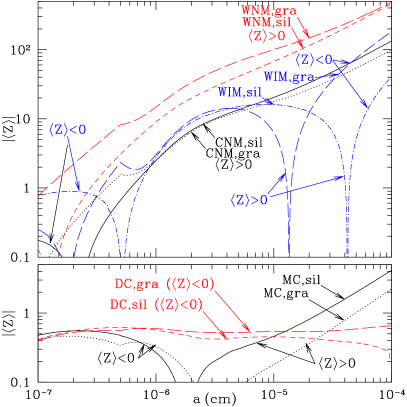
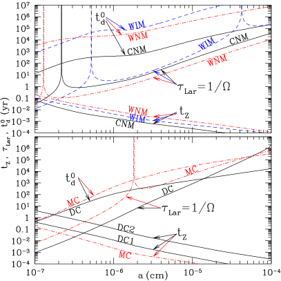
Figure 1: left: $|\langle Z\rangle|$ as a function of grain radius for carbon and silicate grains in 6 different environments: CNM,WNM,WIM,MC, DC1 and DC2. $|\langle Z\rangle|$ distribution is the same for DC1 and DC2, which are referred to as DC in the plot. right: the gas-drag time $t_{d}^{0}$ for subsonic grains, the Larmor time $\tau_{\rm Lar}$, and the charge relaxation time scale, $t_{Z}$, all as a function of grain size for silicate grains in the 6 different environments.

4 Grain Motions arising from hydro-drag

In hydrodynamic turbulence, the grain motions are caused by the frictional interaction with the gas. On large scales grains are coupled with the ambient gas, and the fluctuating gas motions mostly cause an overall advection of the grains with the gas (Draine 1985). At small scales grains are decoupled. The largest velocity difference occurs on the largest scale where grains are still decoupled. Thus the characteristic velocity of a grain with respect to the gas corresponds to the velocity dispersion of the turbulence on the time scale $t_{d}$. In the MHD case, the charged grains are subject to electromagnetic forces. If $\tau_{\rm Lar}>t_{d}$, the grain does not feel the magnetic field. Otherwise, if $\tau_{\rm Lar}<t_{d}$, grain perpendicular motions are constrained by the magnetic field.

As Alfvénic turbulence is anisotropic, it is convenient to consider separately grain motions parallel and perpendicular to the magnetic field. The motions perpendicular to the magnetic field are influenced by Alfvén modes, while those parallel to the magnetic field are subjected to the magnetosonic modes. According to $\S 2$, the perpendicular velocity field scales as $v_{k}\approx V\left(\tau_{k}/\tau_{max}\right)^{1/2},$ where $\tau_{max}=L/V$ is the time-scale on the injection scale.

If the Larmor time $\tau_{\rm Lar}<\tau_{d}$, grain perpendicular motions are constrained by the magnetic field. In this case, grains have a velocity dispersion determined by the turbulence eddy whose turnover period is $\sim\tau_{\rm Lar}$, while grains move with the magnetic field on longer time scales. Since the turbulence velocity grows with the eddy size, the largest velocity difference occurs on the largest scale where grains are still decoupled. Thus, following the approach in Draine (1985), we can estimate the characteristic grain velocity relative to the fluid as the velocity of the eddy with a turnover time equal to $\tau_{\rm Lar}$,

$$v_{\perp}(a) = {\frac{V^{3/2}}{L^{1/2}}}(\rho_{gr})^{1/2}\left({\frac{8\pi^{2}c}{3qB}}\right)^{1/2}a^{3/2}$$ (2)

$$= 0.9\times 10^{5}\,{\rm cm}\,{\rm s}^{-1}(V_{5}a_{5})^{3/2}/(ZL_{10}B_{\mu})^{1/2},$$

in which $V_{5}=V/10^{5}\,{\rm cm}\,{\rm s}^{-1}$, $a_{5}=a/10^{-5}$cm, $Z=q/e$, $L_{10}=L/10$pc, $B_{\mu}=B/1\mu$G, and $\rho_{gr}$ is the mass density of grain. We adopt $\rho_{gr}=3.8$g cm^-3 for silicate grains and $\rho_{gr}=2$gcm^-3 for carbonaceous grains.

Grain motions parallel to the magnetic field are induced by the compressive component of the slow mode with $v_{\parallel}\approx V\times\tau_{k}/\tau_{max}$. For grain motions parallel to the magnetic field the Larmor precession is unimportant and the gas-grain coupling takes place on the translational drag time $t_{d}$. The drag time due to collisions with atoms $t^{\prime}_{d}=(a\rho_{gr}/n_{n})(\pi/8m_{n}k_{B}T)^{1/2}$, where $a$ is the grain size, $m_{n}$ is the mass of gas species, $T$ is the temperature, is essentially the time for collision with the mass of gas equal to the mass of grain. The ion-grain cross-section due to long-range Coulomb force is larger than the atom-grain cross-section . For subsonic motions, the effective drag time $t_{d}^{0}=t^{\prime}_{d}/\alpha$, where (Draine & Salpeter 1979)

$$\alpha = \left[1+\frac{n_{\rm H}}{2n_{n}}\sum_{i}x_{i}\left(\frac{m_{i}}{m_{n}}\right)^{1/2}\sum_{Z}f_{Z}\left(\frac{Ze^{2}}{ak_{B}T}\right)^{2}\right.$$ (3)

$$\left.\ln\left[\frac{3(k_{B}T)^{3/2}}{2e^{3}|Z|(\pi xn_{\rm H})^{1/2}}\right]\right]^{-1},$$

where $x_{i}$ is the abundance, relative to hydrogen, of ion $i$ with mass $m_{i}$, $x=\sum_{i}x_{i}$, and $f_{Z}$ is the probability of the grain being in charge state $Z$.

The characteristic velocity of grain motions along the magnetic field is approximately equal to the parallel turbulent velocity of eddies with turnover time equal to $t_{d}$

$$v_{\parallel}(a) = \alpha^{-1}{\frac{V^{2}}{L}}\left(\frac{\rho_{gr}}{4n_{n}}\right)({\frac{2\pi}{m_{n}k_{B}T}})^{1/2}a$$ (4)

$$= (3.8\times 10^{5}\,{\rm cm}/s)\alpha^{-1}V_{5}^{2}a_{5}/(nL_{10}T_{100}^{1/2}),$$

where $T_{100}=T/100$K. Eq. (4) is valid for subsonic motion, $v<(k_{B}T/m_{n})^{1/2}$.

When the grain velocity $v$ relative to the gas becomes supersonic (Purcell 1969), the gas drag time $t_{d}\approx t_{d}^{0}/(1+(9\pi/128)v^{2}/C_{s}^{2})^{1/2}$.

When $\tau_{\rm Lar}>t_{d}$, grains are no longer tied to the magnetic field. Since at a given scale, the largest velocity dispersion is perpendicular to the magnetic field direction, the velocity gradient over the grain mean free path is maximal in the direction perpendicular to the magnetic field direction. The corresponding scaling is analogous to the hydrodynamic case, which was discussed in Draine (1985):

$$v(a) = {\frac{V^{3/2}}{L^{1/2}}}t_{d}^{1/2}$$ (5)

$$= \alpha^{-1/2}{\frac{V^{3/2}}{L^{1/2}}}\left(\frac{\rho_{gr}}{4n_{n}}\right)^{1/2}\left({\frac{2\pi}{m_{n}k_{B}T}}\right)^{1/4}a^{1/2}.$$

It is easy to see that the grain motions get modified when the damping time scale of the turbulence $\tau_{c}$ is longer than either $t_{d}$ or $\tau_{\rm Lar}$. In this case, a grain samples only a part of the eddy before gaining the velocity of the ambient gas. In a turbulent medium, the shear rate $dv/dl$ increases with the decrease of eddy size. Thus for $\tau_{c}>\max\{t_{d},\tau_{\rm Lar}\}$, these smallest available eddies are the most important for grain acceleration. Consider first the perpendicular motions. If $v_{c}$ is the velocity of the critically damped eddy, the distance traveled by the grain is $\bigtriangleup l\sim v_{c}\times\min\{t_{d},\tau_{\rm Lar}\}$. The shear rate $dv/dl$ perpendicular to the magnetic field is $\tau_{k}^{-1}$. Thus the grain experiences the velocity difference in the direction perpendicular to the magnetic field

$$v_{\perp}\sim\bigtriangleup l\times\frac{dv}{dl}\sim\frac{v_{c}}{\tau_{c}}\times\min\{t_{d},\tau_{\rm Lar}\}.$$ (6)

For the parallel motions, $\bigtriangleup l\sim v_{c}\times t_{d}$. From the critical balance in the GS95 model $k_{\parallel}V_{A}\sim k_{\perp}v_{\perp}=\tau_{k}^{-1}$, the largest shear rate along the magnetic field should be $dv/dl=v_{c}k_{\parallel}\sim v_{c}/(V_{A}\tau_{c})$. Therefore, in the parallel direction, the grain experiences a velocity difference $V_{A}/v_{c}$ times smaller, i.e.,

$$v_{\parallel}\sim\frac{v_{c}^{2}}{V_{A}}\times\frac{t_{d}}{\tau_{c}}.$$

The velocity dispersion induced by the compressional motion associated with the fast modes also causes motion relative to the ambient gas. The velocity fluctuation for fast modes scales as $v_{k}\propto k^{-1/4}\propto\omega^{-1/4}$, where $\omega$ is the frequency of fast modes. From similar considerations, we know that grains get velocity dispersions during $\min\{\tau_{\rm Lar},t_{d}\}$,i.e. , $v\simeq V(\min\{\tau_{\rm Lar},t_{d}\}/\tau_{max})^{1/4}$. Grains with $\min\{\tau_{\rm Lar},t_{d}\}<\tau_{c}$, have reduced velocities $v\sim v_{c}\times\tau_{\rm Lar}/\tau_{c}\sim V(\tau_{\rm Lar}/\tau_{max})^{1/4}(\tau_{\rm Lar}/\tau_{c})^{3/4}$, where $v_{c}$ is the velocity of turbulence at the damping scale. From the scaling, we see that the decoupling from fast modes always brings larger velocity dispersions to grains than Alfvén modes ($v_{k}\propto k^{-1/3}$) except for the situation when Alfvén modes dominate MHD turbulence. The velocity fluctuations associated with fast modes are always in the direction perpendicular to $\mathbf{B}$ in low $\beta$ media (see Appendix D). Thus the grain velocities are also perpendicular to $\mathbf{B}$. In high $\beta$ media, grains can have velocity dispersion in any direction as the velocity dispersions of fast modes are longitudinal, i.e., along $\mathbf{k}$.

5 Acceleration of Grains by Gyroresonance

Gyroresonance acceleration of charged grains by a spectrum of MHD waves decomposed into incompressive Alfvénic, and compressive fast and slow modes (see CL02) was first described in YL02. The resonance happens when $\omega-k_{\parallel}v\mu=n\Omega$, ($n=0,\pm 1,\pm 2...$), where $\omega$ is the wave frequency, $k_{\parallel}$ is the parallel component of wave vector k along the magnetic field, $v$ is the grain velocity, $\mu$ is the cosine of the grain pitch angle relative to the magnetic field, and $\Omega$ is the Larmor frequency of the grain. There are two main types of resonant interactions: gyroresonance acceleration and transit acceleration. Transit acceleration ($n=0$) requires longitudinal motions and only operates with compressive modes. It happens when $k_{\parallel}v\mu=\omega$, which requires particle speed to be super-Alfvénic $v>V_{f}\geq V_{A}$. Although this condition is partially relieved owing to resonance broadening (see Yan & Lazarian 2004), transit acceleration of low speed grains is marginal because sub-Alfvénic particles can hardly catch up with the moving magnetic mirror.

How can we understand grain gyroresonance? Gyroresonance occurs when the Doppler shifted frequency of the wave in the grain’s guiding center rest frame $\omega_{gc}=\omega-k_{\parallel}v\mu$ is a multiple of the grain gyrofrequency. For low speed grains, we only need to consider the resonance at $n=1.$ The gyroresonance changes both the direction and absolute value of the grain’s momentum (i.e., scatters and accelerates the grain). The efficiency of the two processes for charged grains can be described by the Fokker-Planck coefficients $D_{\mu\mu}$ and $D_{pp}/p^{2}$, where $p$ is the grain momentum. The ratio of the two rates depends on the ratio of the grain velocity and the Alfvén speed and pitch angle, $p^{2}D_{\mu\mu}/D_{pp}=[(v\zeta/V_{A})+\mu]^{2}$, where $\zeta=1$ for Alfvén waves and $\zeta=k_{\parallel}/k$ for fast modes (see Appendix B). We see that the scattering is less efficient for sub-Alfvénic grains unless most grains move parallel to the magnetic field. We shall show later that as the result of acceleration, $\mu$ will tend to 0. Therefore in the zeroth order approximation, we ignore the effect of scattering and assume that the pitch angle cosine $\mu$ does not change while a grain is accelerated. In this case, the Fokker-Planck equation, which describes the diffusion of grains in momentum space, can be simplified (see Pryadko & Petrosian 1997):

$$\frac{\partial f^{\mu}}{\partial t}+v\mu\frac{\partial f^{\mu}}{\partial z}=\frac{1}{p^{2}}\frac{\partial}{\partial p}p^{2}D_{pp}(\mu)\frac{\partial f^{\mu}}{\partial p},$$ (7)

where $f$ is the distribution function. Apart from acceleration, a grain is subjected to gaseous friction. Thus we describe the stochastic acceleration by the Brownian motion equation:

$$m\frac{dv}{dt}=-\frac{v}{S}+Y,$$ (8)

where $m$ is the grain mass, $Y$ is the stochastic acceleration force, $S=t_{d}/m$ is the mobility coefficient.

If we multiply equation(8) by $v$, and take the ensemble average, we obtain

$$m\frac{d\langle v^{2}\rangle}{dt}=-\frac{\langle v^{2}\rangle}{S}+\langle\dot{\epsilon}^{\mu}\rangle.$$ (9)

The steady solution is achieved when the derivative on the left-hand is zero. Following an approach similar to that in Melrose (1980), we can get from Eq.(7) the energy gain rate for the grain with pitch angle $\mu$

$$\langle\dot{\epsilon}^{\mu}\rangle=\frac{1}{p^{2}}\frac{\partial}{\partial p}(vp^{2}D_{pp}(\mu)).$$ (10)

The Fokker-Planck coefficient $D_{pp}(\mu)$ is calculated below.

YL03 employed quasi-linear theory (QLT) to obtain $D_{pp}(\mu)$ (see also YL02 and Appendix B) :

$$D_{pp}(\mu) = {\frac{\pi\Omega^{2}(1-\mu^{2})p^{2}V_{A}^{2}}{2v^{2}}}\Big{\{}\int dk^{3}\frac{\tau_{k}^{-1}}{\tau_{k}^{-2}+(\omega-k_{\parallel}v\mu-\Omega)^{2}}$$ (11)

$$\Big{[}(J_{2}^{2}({\frac{k_{\perp}v_{\perp}}{\Omega}})M_{\mathcal{RR}}({\mathbf{k}}))+J_{0}^{2}({\frac{k_{\perp}v_{\perp}}{\Omega}})M_{\mathcal{LL}}({\mathbf{k}}))$$

$$- J_{2}({\frac{k_{\perp}v_{\perp}}{\Omega}})J_{0}({\frac{k_{\perp}v_{\perp}}{\Omega}})$$

$$(e^{i2\phi}M_{\mathcal{RL}}({\mathbf{k}})+e^{-i2\phi}M_{\mathcal{LR}}({\mathbf{k}}))\Big{]}\Big{\}}.$$

However, we should not integrate over all $k$ because the contribution from large scales is spurious (see discussion in YL02). This contribution stems from the fact that in QLT, an unperturbed grain orbit is assumed, which results in non-conservation of the adiabatic invariant $\xi=mv_{\perp}^{2}/2B_{0}$. Noticing that the adiabatic invariant is conserved when the electromagnetic field varies on a time scale longer than $\Omega^{-1}$, we truncate our integral range, namely, integrate from $k_{res}$ instead of the injection scale $L^{-1}$. For Alfvénic turbulence $\omega=|k_{\parallel}|V_{A}$, the resonant scale corresponds to $|k_{\parallel,res}|=\Omega/|V_{A}-v\mu|.$ For fast modes, the resonant scale is $k_{res}=\Omega/|V_{f}-v\mu\cos\theta|$, where $\cos\theta=k_{\parallel}/k$. The upper limit of the integral $k_{c}$ is set by the dissipation of the MHD turbulence, which varies with the medium.

Integrating from $k_{res}$ to $k_{c}$, we obtain from Eq.(11) and (10) the energy gain rate $\dot{\epsilon}$ as a function of $v$ and $\mu$. Then with $\dot{\epsilon}$ known, we estimate the grain acceleration. Solving Eq.(9) iteratively, we obtain the grain velocity as a function of time. We check that the grain velocities converge to a constant value after the drag time. As $\dot{\epsilon}$ increases with pitch angle, grains gain the maximum velocities perpendicular to the magnetic field and therefore the averaged $\mu$ decreases. This is understandable since the electric field, which accelerates the grain, is in the direction perpendicular to the magnetic field.

6 Grain motions in the ISM

Here we apply our results to various idealized phases of the interstellar medium.

ISM	CNM	WNM	WIM	MC	DC1	DC2
T(K)	100	6000	8000	25	10
$n_{\rm H}$(cm-3)	30	0.3	0.1	300	$10^{4}$
$n_{e}$(cm-3)	0.03	0.03	0.0991	0.03	0.01	0.001
$G_{UV}$	1	1	1	0.1	0.01	0.001
B($\mu$G)	6	5.8	3.35	11	80
L(pc)	0.64*	100	100	1	1
$V=V_{A}$(km/s)	2*	20	20	1.2	1.5
damping	neutral-ion	neutral-ion	collisional	neutral-ion	ion-neutral decoupling
$k_{c}(\,{\rm cm}^{-1})$	$7\times 10^{-15}$	$4\times 10^{-17}$	$NA$	$4.5\times 10^{-14}$	$5.3\times 10^{-15}$	$5.3\times 10^{-17}$

Table 1: The parameters of idealized ISM phases and relevant damping. Among them, $n_{\rm H}$ is the number density of H, $n_{e}$ is the number density of electron, $G_{UV}$ is the UV intensity scale factor, L is the injection scale of fast modes, V is the injection velocity. The dominant damping mechanisms for fast modes are given with the corresponding damping timescale $\tau_{c}$. CNM=cold neutral medium, WNM=warm neutral medium, WIM=warm ionized medium, MC=molecular cloud, DC=dark cloud. * See text for the explanation of smaller L and V for CNM.

First consider a typical cold neutral medium (CNM), $T=100$K, $n_{\rm H}=30$cm${}^{-3},$ $n_{e}=0.045$cm^-3, $B=6\mu$G, with corresponding $v_{A}=2$ km/s and $\beta\sim 0.4$.

Our treatment of MHD turbulence requires that fluid velocities are smaller than the Alfvén speed. Therefore we assume that the injection of energy happens at an effective injection scale $L$ where equipartition between magnetic and kinetic energies, i.e., $V=V_{A}$, occurs. This effective injection scale can be different from the actual scale at which energy is injected. For instance, if we assume that the velocity dispersion at the scale $l=10$pc is 5km/s, this means that turbulence in the CNM is super-Alfvénic at this scale. The turbulence then follows a hydrodynamic cascade down to a scale $L\approx 0.64$pc where the turbulent velocity becomes equal to $V_{A}=2$km/s; we identify this as the effective “injection scale” $L$with injection velocity $V=V_{A}=2$km/s. Alternatively, it is possible that the turbulence at large scales proceeds in tenuous warm media with Alfvén speed larger or equal to 5km/s. Nevertheless, the statistics of fast modes will not be changed in the CNM.

In partially ionized media, the damping is dominated by the viscosity arising from neutrals. The turbulence is assumed damped when its cascading time scale $\tau_{k}=t_{damp}$; this defines the cutoff scale $k_{\parallel,c}=4\times 10^{-16}$cm^-1 for Alfvén modes and $k_{c}=7\times 10^{-15}$cm^-1 for fast modes (see Appendix A). Assuming that the grain velocities are smaller than the phase speed of fast modes, we find that the prerequisite for gyroresonance $k_{c}>k_{res}$ is the same as $\tau_{\rm Lar}>\tau_{c},$ the condition for effective hydro drag (see Fig.1). For a silicate grain, the critical grain size $a_{c}\approx 4\times 10^{-6}$cm for fast modes and $a_{c}\approx 10^{-5}$cm for Alfvén modes. Grains smaller than the critical size are not effectively accelerated by the corresponding turbulent mode.

The CNM is a low $\beta$ medium, so the correlation tensors for the low $\beta$ case are applied. As has been discussed in YL02, the interactions with Alfvén modes are less efficient than those with fast modes because of the anisotropy of Alfvén modes. Thus we shall consider only fast modes for later calculations. The gyroresonance with fast modes in the CNM can accelerate grains to supersonic velocities. $\dot{\epsilon}^{\mu}$ increases with pitch angle. If we average $\dot{\epsilon}$ over $\mu$, we will get mean velocities which are smaller than the maximum values by less than $20\%$. In Fig.1 we plot the velocity of grains with pitch angle equal to $90^{o}$ as a function of grain size since all the mechanisms preferentially accelerate grains in this direction.

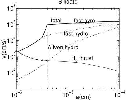
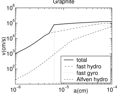
Figure 2: Relative velocities as a function of radii (solid line) in CNM, left: for silicate grains, right: for graphite grains. The dotted lines represent the gyroresonance with fast modes. Gyroresonance works only for large grains owing to the cutoff by viscous damping. The cutoff scales for fast and Alfvén modes are different due to their different scalings and the anisotropy of Alfvén modes. The dashed lines are the result from hydro drag by Alfvén modes (see LY02), the dashdot lines represent the hydro drag by fast modes. Contributions from different mechanisms are approximately additive in squares, i.e., $v_{tot}^{2}=\Sigma_{i}v_{i}^{2}$ (heavy solid lines). The grain velocity driven by H₂ formation (dashdot line) is plotted to illustrate the issue of grain segregation in CNM (see text). The part marked by open circles is nonphysical because thermal flipping is not taken into account.

For the warm neutral medium (WNM), $T=6000$K, $n_{H}=0.3$cm^-3, $n_{e}=0.03$cm^-3, $B=5.8\mu$G. Assume the velocity dispersion $V=V_{A}=20$km/s at the injection scale $L=100$pc. Turbulence is mainly subjected to neutral-ion damping. The fast modes are cut off at $k_{c}=4\times 10^{-17}\,{\rm cm}^{-1}$ (see Appendix A). Comparing $k_{c}$ with $k_{res}$, we find $a_{c}\approx 2\times 10^{-5}$cm for silicate grains. The WNM has $\beta\approx 0.25$, so we use the tensor given in Eq.(B28) for fast modes. Integrating from $k_{res}$ to $k_{c}$ and solving Eq.(9), we obtain grain velocities. The maximum values are shown in Fig.2. We see large grains can be accelerated to supersonic speeds. The fact that these grains approach the Alfvén speed makes our approximation that acceleration dominates scattering less accurate, but the result is correct within a factor of unity. Smaller grains are accelerated only by the hydro drag, which is far less effective.

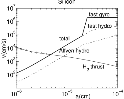
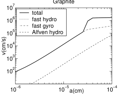
Figure 3: Same as Fig2, but in the WNM.

The warm ionized medium (WIM) has $T=8000$K, $n_{e}=0.1\,{\rm cm}^{-3}$, $B=3.35\mu$G, with corresponding $\beta\sim 0.33$. The injection scale and speed are the same as in the WNM. The WIM is fully ionized and in low $\beta$ regime. Fast modes, in this case, are mainly affected by collisional damping. This damping increases with $\theta$, and doesn’t exist for parallel modes (see Appendix A). Thus there are always modes interacting with grains though the energy available is less at smaller scales. Following the same routine as above, we get the grain velocities. We see from Fig.4 the nonmonotonic variation of grain velocity with the size. This arises from the fact that the charging for grains in the WIM has a complex dependence on grain size (see also Fig.1a).

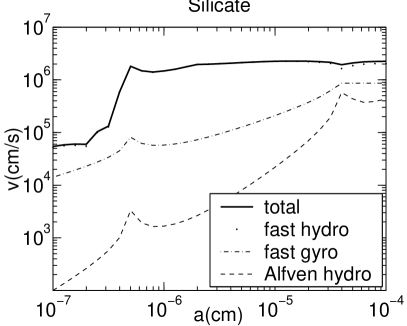
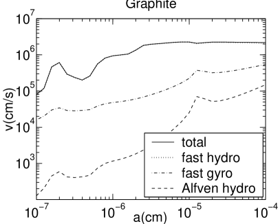
Figure 4: Same as Fig.2, but in the WIM. The oscillations in these curves are due to the variation in charging of grains.

Molecular cloud (MC) gas has $T=25$K, $n_{\rm H}=300$cm^-3, and we adopt a magnetic field strength $B=11\mu$G as suggested by observations (Crutcher 1999), corresponding to Alfvén speed $V_{A}=1.2{\rm\,kms\,}^{-1}$. The injection scale is taken to be $L=1$pc and the injection velocity is $V=V_{A}$. The damping scale (see Appendix A) of the turbulence is $k_{c}=4.5\times 10^{-14}{\rm\,cm\,}^{-1}$, corresponding to resonant scales of silicate grains with $a=8\times 10^{-7}$cm. By following the same procedure, we obtain the grain velocity distribution as shown in Fig.5.

We consider a typical dark cloud (DC) with $T=10$K, $n_{\rm{H}}=10^{4}$cm^-3, and $B\sim 80\mu$G, corresponding to $V_{A}=1.5{\rm km\,s}^{-1}$. The injection scale $L=1$pc and velocity $V=V_{A}$. The ionization in DC is so low that the fluid becomes decoupled in the middle of the cascade, where the ion-neutral collision rate $t_{ni}^{-1}$ per neutral is equal to the turbulence decay rate $\tau_{k}^{-1}$. Below this decoupling scale, neutrals will not follow ions and magnetic fields, and the turbulence becomes hydrodynamic. In view of the uncertainty of the cosmic-ray ionization rate, we adopt two models DC1 and DC2 with electron densities $n_{e}=0.01\,{\rm cm}^{-3}$ and $n_{e}=0.001\,{\rm cm}^{-3}$. The grain charge distribution is the same for both DC1 and DC2, because we assume the same $G_{UV}/n_{e}$. The main difference is the decoupling scale of the MHD cascade. Combining Eq.(1) and Eq.(A2), we can obtain the decoupling scales $k_{c}=5.3\times 10^{-15}\,{\rm cm}^{-1}$ for DC1 and $k_{c}=5.3\times 10^{-17}\,{\rm cm}^{-1}$ for DC2, corresponding to silicate grain size $a_{c}\approx 3\times 10^{-6}$cm for DC1 and $a_{c}\approx 2\times 10^{-5}\,{\rm cm}$ for DC2. By following the same procedure, we obtain the grain velocity distribution as shown in Fig. 6 and Fig. 7.

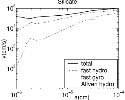
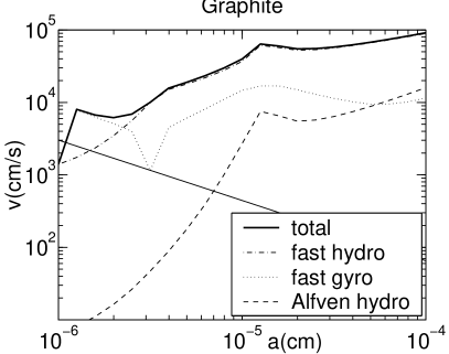
Figure 5: Same as Fig.4, but in the MC.

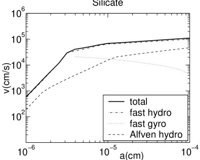
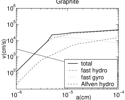
Figure 6: Same as Fig.2, but in DC1.

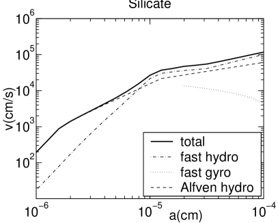
Figure 7: Same as Fig.2, but in DC2.

It is shown in Fig. 5,6&7 that the acceleration by gyroresonance in both MC and DC is not as effective as in the lower density media, for two reasons. First, the low levels of UV and low temperatures result in reduced grain charge (see Fig. 1a). Secondly, because of the increased density, the drag time $t_{d}$ is reduced.

The grain velocities in CNM found here are smaller than in an earlier calculation (see YL03) because we adopt smaller values for magnetic field $B$ and injection velocity $V$.

It should be noted that the strength of magnetic fields in the ISM is still somewhat uncertain and may vary from place to place. We adopted a particular set of values in above calculations. How would the results vary as the magnetic field strength varies? First of all, we know that the critical condition for acceleration is $k_{res}>k_{d}$: grains with $k_{res}<k_{d}$ cannot be accelerated. Thus the cutoff grain radius $a_{c}$ varies with the medium, $a_{c}\approx[3q(a_{c})\tau_{c}B/4\pi\rho]^{1/3}$; grains with $a<a_{c}$ are not subject to gyroresonant acceleration.

The magnitude of the velocity is a complex function of the magnetic field. For illustration, in Fig.7 we show the grain velocities calculated for magnetic fields a factor of 3 stronger or weaker than the values in Table 1 for the CNM and DC1 environment. Since the hydro drag by fast modes decreases with the magnetic field, the relative importance of gyroresonance and hydro drag depends on the magnitude of the magnetic field. In magnetically dominant regions, gyroresonance is dominant. In weakly magnetized regions, the frictional drag provides the highest acceleration rate. The injection scale is another uncertain parameter, but the grain velocity is not so sensitive to it provided that the injection scale is much larger than the damping scale.

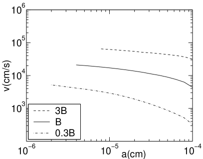
Figure 8: Relative velocities gained from gyroresonance as a function of radii for different magnetic field strength, left: in CNM, right: in DC1. Solid lines are the results for the precedent values of magnetic field. Dashed lines refer to the results with 3 times stronger magnetic field. Dash-dot lines represent the cases with 3 times weaker magnetic field.

7 Discussion

Shattering and Coagulation

With the grain relative velocities known, we can make predictions for grain shattering and coagulation. For shattering, we adopt the Jones et al. (1996) results, namely, for equal-sized particles the shattering threshold is 2.7km/s for silicate grains and 1.2km/s for carbonaceous grains. The critical sticking velocity was given by Chokshi et al. (1993) (see also Dominik & Tielens 1997):

$$v_{cr}=2.14F_{\rm stick}\left[\frac{a_{1}^{3}+a_{2}^{3}}{(a_{1}+a_{2})^{3}}\right]^{1/2}\frac{\gamma^{5/6}}{E^{1/3}R^{5/6}\rho^{1/2}},$$

is the maximum relative velocity for coagulation of equal-size spherical grains, where $\gamma$ is the surface energy per unit area, $R=a_{1}a_{2}/(a_{1}+a_{2})$ is the reduced radius of the grains and $E$ is related to Poisson’s ratio $\nu_{i}$ and Young’s modulus $E_{i}$ by $1/E=[(1-\nu_{1})^{2}/E_{1}+(1-\nu_{2})^{2}/E_{2}]$ and we have introduced a factor $F_{stick}\approx 10$ since the experimental work by Blum (2000) shows that the critical velocity is an order of magnitude higher than the theoretical estimate of Chokshi et al. We use $\gamma$, $E$ and $\nu$ for SiO₂ and graphite from Table 1 of Dominik & Tielens (1997), and consider collisions between equal-size grains ($a_{1}\approx a_{2}$). Comparing these critical velocities with the velocity curve we obtained for various media, we can get the corresponding critical size for each of them (see Table 2).

ISM	CNM		WNM		WIM		DC1		DC2
Material	sil.	C	sil.	C	sil.	C	sil.	C	sil.	C
Shattering ($\mu$m)	NA	NA	$>0.2$	$>0.2$	$>0.003$	$>0.001$	NA	NA	NA	NA
Coagulation ($\mu$m)	$<0.01$	$<0.02$	$<0.02$	$<0.04$	NA	NA	$\lesssim 0.01$	$<0.02$	$<0.02$	$<0.04$

Table 2: Size ranges for shattering and coagulation in different medium. NA=not applicable.

Correlation between turbulence and grain sizes

The grain velocities are strongly dependent on the maximal velocity of turbulence $V$ at the injection scale, which is highly uncertain. The critical coagulation and shattering sizes thus also depend on the amplitude of the turbulence. Variations in the level of turbulence could lead to regional differences in the grain size distribution.

Elements in cosmic rays

It has been shown that the composition of galactic cosmic rays appears to be correlated with elemental volatility (Ellison, Drury & Meyer 1997). The more refractory elements are systematically overabundant relative to the more volatile ones. This suggests that the material locked in grains must be accelerated more efficiently than gas-phase ions (Epstein 1980; Ellison, Drury & Meyer 1997). The stochastic acceleration of grains, in this case, can act as a preacceleration mechanism. The ions released from the grains in the shock by sputtering or in grain-grain collisions can then be further accelerated in the shock, and explain the overabundance of refractory elements in galactic cosmic rays.

Heavy Element Depletion and Grain Alignment

Our results indicate that grains can become supersonic through interaction with fast modes. Grains moving with velocities larger that those of heavy ions could sweep up heavy elements which may be advantageous from the point of explaining observations (Wakker & Mathis 2000). Our calculations show that while such velocities are readily achievable, the sign of charging may present a problem for such “vacuum cleaning” of the ISM. For instance, silicate grains in MC can be accelerated to $\gtrsim 4\times 10^{4}$ cm/s, which is larger than the thermal speed of heavy ion. Therefore the capture rate for ions by positively charged grains ($\lesssim 2\times 10^{-6}$ cm) would be increased. Grains smaller than $2\times 10^{-6}$ cm will be negatively charged in the MC. For such grains the cross section for Coulomb capture of ions will decrease. If such small grains retain captured ions, this would result in a decrease of the rate of depletion of metals on grains. The actual rates of depletion on fast moving grains are important and will be identified elsewhere for particular phases of the ISM.

Grains moving supersonically can be aligned mechanically (see a review by Lazarian 2003 and references therein). As pointed out earlier, the scattering is not efficient for slowly moving grains so that we may ignore the effect of scattering on the pitch angle. Since the acceleration of grains increases with the pitch angle of the grain(see Eq.(10) and (11)), the supersonic grains will tend to have large pitch angles. As first discussed by Gold (1952), gas drag acting on these grains will tend to cause them to spin with angular momenta perpendicular to their motion, and therefore tending to be parallel to the magnetic field direction. Dissipational processes will tend to orient the spinning grains with their long axes perpendicular to their angular momentum, resulting in grain alignment with long axes perpendicular to the magnetic direction.

Grain Segregation and Turbulent Mixing

Our results are also relevant to grain segregation. Grains are the major carrier of heavy elements in the ISM. The issue of grain segregation may have significant influence on the ISM metalicity. Subjected to external forcing (WD01, Ciolek and Mouschovias 1996), grains gain size-dependent velocities with respect to gas. WD01 considered the forces on dust grains exposed to anisotropic interstellar radiation fields, including photoelectric emission, photodesorption, and radiation pressure, and calculated the drift velocity for grains of different sizes. The velocities they got for silicate grains in the CNM range from $0.1$cm/s to $10^{3}$cm/s. Grains can move along magnetic field lines due to the uncompensated forces, e.g. due to active sites of H₂ formation (see P79; Lazarian & Yan 2002b) Fig. 2a shows that the turbulence produces larger velocity dispersions. Those velocities are preferentially perpendicular to magnetic field, but in many cases the dispersion of velocities parallel to magnetic field will be comparable to the regular velocities above. This dispersion stems from both the fact that the transpositions of matter by fast modes are not exactly perpendicular to magnetic field (see plot in Lazarian & Yan 2002b) and due to randomization of directions of grain velocities by magnetized turbulence (YL03).

More important is that if reconnection in turbulent medium is fast (see Lazarian & Vishniac 1999, Lazarian et al. 2004), the mixing of grains over large scales is provided by turbulent diffusivity $\sim VL/4$. Usually it was assumed that the magnetic fields strongly suppress the diffusion of charged species perpendicular to their directions. However, this assumption is questionable if we notice that motions perpendicular to the local magnetic field are hydrodynamic to high order as suggested by Cho, Lazarian & Vishniac (2002). Recent work by Cho et al. (2003) found that the diffusion processes in MHD turbulence are almost as effective as in the hydrodynamic case if the mean magnetic field is weak or moderately strong (i.e., $B\leq$ the equipartition value) which would imply that grains can be mixed by the MHD turbulence. Lazarian & Yan (2003) therefore concluded that the segregation of very small and large grains speculated in de Oliveira-Costa et al. (2002) is unlikely to happen for typical interstellar conditions.

8 Summary

We have calculated the relative motions of dust grains in a magnetized turbulent fluid. It has been known for decades that turbulence can give rise to significant grain-grain velocities. However, earlier treatments disregarded the magnetic field and used Kolmogorov turbulence. Magnetohydrodynamic (MHD) turbulence includes both fluid motions and magnetic fluctuations. While the fluid motions bring about decoupled motions to grains, the electromagnetic fluctuations can accelerate grains through resonant interactions.

Calculations of grain relative motion are made for different phases of the ISM with realistic grain charging, and with turbulence that is consistent with the velocity dispersions observed in interstellar gas. We account for the cutoff of the turbulence from various damping processes. We show that fast modes dominate grain acceleration, and can drive grains to supersonic velocities. Grains are also scattered by gyroresonance interactions. The scattering rate is less efficient than acceleration for grains moving with sub-Alfvénic velocities.

Since the grains are preferentially accelerated with large pitch angles, the supersonic grains tend to be aligned with long axes perpendicular to the magnetic field.

Gyroresonant acceleration is bound to preaccelerate grains that will then be further accelerated by shocks. Grain-grain collisions and sputtering in the shocks will inject suprathermal ions which can then undergo further acceleration in the shock, potentially accounting for the observed excess of refractory elements in the composition of galactic cosmic rays (e.g., Epstein 1980; Ellison et al. 1997)

Appendix A Damping of MHD waves

Below we summarize the damping processes that we consider in the paper.

Neutral-ion damping

In partially ionized medium, a combination of neutral viscosity and ion-neutral collisional coupling provides damping (see LY02). If the mean free path for a neutral, $l_{n}$, in a partially ionized gas with density $n_{tot}=n_{n}+n_{i}$ is much less than the size of the eddies under consideration, i.e. $l_{n}k\ll 1$, the damping time

$$t_{damp}\sim\nu_{n}^{-1}k^{-2}\sim\left(\frac{n_{tot}}{n_{n}}\right)(l_{n}v_{n})^{-1}k^{-2},$$ (A1)

where $\nu_{n}$ is effective viscosity produced by neutrals, $v_{n}$ is the thermal velocity of the neutrals, and the mean free path of a neutral $l_{n}$ is influenced both by collisions with neutrals and with ions. The rate at which neutrals collide with ions is proportional to the density of ions, while the rate at which neutrals collide with other neutrals is proportional to the density of neutrals. The momentum transfer rate coefficient for neutral-neutral collisions is $\sim 1.7\times 10^{-10}(T/{\rm K})^{0.3}$ cm³ s^-1 (Spitzer 1978), while for neutral-ion collisions it is $\sim{\langle v_{r}\sigma_{in}\rangle}\approx 1.9\times 10^{-9}$ cm³ s^-1 (Draine, Roberge & Dalgarno 1983). Thus collisions with other neutrals dominate for $n_{i}/n_{n}$ less than $\sim 0.09T^{0.3}$.

Effects of charged grains

Magnetic perturbations can get decoupled from the fluid motions because neutrals are imperfectly coupled to the ions in partially ionized medium. The coupling between ions and neutrals is determined by the ion-neutral collisional rate:

$$t_{ni}^{-1}=\frac{m_{i}}{m_{n}+m_{i}}n_{i}\langle v_{r}\sigma_{in}\rangle$$ (A2)

where $v_{r}$ is the ion-neutral relative velocity, $\sigma_{in}$ is the ion-neutral collisional cross section, $m_{i}$ and $m_{n}$ are the typical ion and neutral masses, $n_{i}$ is the ion number density. When the collisional time $t_{ni}$ is equal to the wave period, neutrals are decoupled from magnetic field, and turbulence becomes hydrodynamic. In molecular clouds, grains can take substantial portion of the total charge. The contribution of charged grains to coupling neutrals to magnetic fields depends on grain size spectrum. The ratio of the ion-neutral collisional rate to the grain-neutral collisional rate is (Nishi & Nakano 1991, Elmegreen & Fiebig 1993):

$$\frac{t_{ni}^{-1}}{\langle n_{g}\sigma_{g}\rangle v_{n}}\simeq\cases{0.25n_{4}^{-1/2};&(MRN)\cr 3.3n_{4}^{-1/2};&(MW)\cr},$$ (A3)

where MRN refers to the grain size distribution proposed by Mathis et al. (1977) and MW stands for the distribution suggested by Mathis & Whiffen (1989). From this expression, we can see that ions are always the dominant contribution for the coupling in MC. In DC, the situation will depend on grain size distribution. DC is a denser region where observations favor MW distribution (Elmegreen & Fiebig 1993). Thus presumably the contribution from grains in DC is also subdominant and we neglect it in the main text.

Collisionless damping

The nature of collisionless damping is closely related to the radiation of charged particles in magnetic field. Since the charged particles can emit plasma waves through acceleration (cyclotron radiation) and Cherenkov effect, they also absorb the radiation under the same condition (Ginzburg 1961). The damping rate $\gamma_{d}=\tau_{d}^{-1}$ of the fast modes of frequency $\omega$ for $\beta\ll 1$ and $\theta\sim 1$ (Ginzburg 1961) is

$$\Gamma_{d} = \frac{\sqrt{\pi\beta}}{4}\omega\frac{\sin^{2}\theta}{\cos\theta}\times\left[\sqrt{\frac{m_{e}}{m_{\rm H}}}\exp(-\frac{m_{e}}{m_{\rm H}\beta\cos^{2}\theta})+5\exp(-\frac{1}{\beta\cos^{2}\theta})\right],$$ (A4)

where $m_{e}$ is the electron mass. The exact expression for the damping of fast waves at small $\theta$ was obtained in Stepanov (1958)

$$\Gamma_{d}=\frac{\sqrt{\pi\beta}}{4}\omega\theta^{2}\times\left(1+\frac{\theta^{2}}{\sqrt{\theta^{4}+4\Omega_{i}^{2}/\omega^{2}}}\right)\sqrt{\frac{m_{e}}{m_{\rm H}}}\exp(-\frac{m_{e}}{m_{\rm H}\beta\cos^{2}\theta}).$$

When $\beta\gg 1$ (see Foote & Kulsrud 1979),

$$\Gamma_{L}=\cases{2\omega^{2}/\Omega_{i}&for $k<\Omega_{i}/\beta V_{A}$\cr 2\Omega_{i}/\beta&for $k>\Omega_{i}/\beta V_{A}$\cr}$$ (A5)

where $\Omega_{i}$ is the ion gyrofrequency.

Ion viscosity

In a strong magnetic field ($\Omega_{i}\tau_{i}\gg 1$) the transport of transverse momentum is prohibited by the magnetic field (along $\hat{z}$). Thus transverse viscosity $\eta_{\perp}$ is much smaller than longitudinal viscosity $\eta_{0}$, $\eta_{\perp}\sim\eta_{0}/(\Omega_{i}\tau_{i})^{2}$. Following Braginskii (1965), we can find the damping rate is(see Yan & Lazarian 2004):

$$\Gamma_{ion}=\cases{k_{\perp}^{2}\eta_{0}/6\rho_{i}&for $\beta\ll 1$\cr k^{2}\eta_{0}(1-3\cos^{2}\theta)^{2}/6\rho_{i}&for $\beta\gg 1$\cr}$$ (A6)

For more discussion, see Yan & Lazarian (2004).

Appendix B Fokker-Planck coefficients

In quasi-linear theory (QLT), the effect of MHD waves is studied by calculating the first order corrections to the particle orbit in the uniform magnetic field, and the ensemble-averaging over the statistical properties of the MHD waves (Jokipii 1966, Schlickeiser & Miller 1998). Obtained by applying the QLT to the collisionless Boltzmann-Vlasov equation, the Fokker-Planck equation is generally used to describe the evolvement of the gyrophase-averaged particle distribution,

$$\frac{\partial f}{\partial t}=\frac{\partial}{\partial\mu}\left(D_{\mu\mu}\frac{\partial f}{\partial\mu}+D_{\mu p}\frac{\partial f}{\partial p}\right)+\frac{1}{p^{2}}\frac{\partial}{\partial p}\left[p^{2}\left(D_{\mu p}\frac{\partial f}{\partial\mu}+D_{pp}\frac{\partial f}{\partial p}\right)\right],$$

where $p$ is the particle momentum. The Fokker-Planck coefficients $D_{\mu\mu},D_{\mu p},D_{pp}$ are the fundamental physical parameter for measuring the stochastic interactions,

$$\left(\begin{array}[]{c}D_{\mu\mu}\\ D_{\mu p}\\ D_{pp}\end{array}\right) = {\frac{\pi\Omega^{2}(1-\mu^{2})}{2}}\int_{\bf k_{min}}^{\bf k_{max}}dk^{3}\frac{\tau_{k}^{-1}}{\tau_{k}^{-2}+(\omega-k_{\parallel}v\mu-\Omega)^{2}}\left(\begin{array}[]{c}\left(1+\frac{\mu V_{ph}}{v\zeta}\right)^{2}\\ \left(1+\frac{\mu V_{ph}}{v\zeta}\right)mV_{A}\\ m^{2}V_{A}^{2}\end{array}\right)$$ (B11)

$$\left\{(J_{2}^{2}({\frac{k_{\perp}v_{\perp}}{\Omega}})+J_{0}^{2}({\frac{k_{\perp}v_{\perp}}{\Omega}}))\left[\begin{array}[]{c}M_{{\mathcal{RR}}}({\mathbf{k}})+M_{{\mathcal{LL}}}({\mathbf{k}})\\ -C_{{\mathcal{RR}}}({\mathbf{k}})-C_{{\mathcal{LL}}}({\mathbf{k}})\\ K_{{\mathcal{RR}}}({\mathbf{k}})+K_{{\mathcal{LL}}}({\mathbf{k}})\end{array}\right]\right.$$

$$- 2J_{2}({\frac{k_{\perp}v_{\perp}}{\Omega}})J_{0}({\frac{k_{\perp}v_{\perp}}{\Omega}})\left.\left[e^{i2\phi}\left[\begin{array}[]{c}M_{{\mathcal{RL}}}({\mathbf{k}})\\ -C_{{\mathcal{RL}}}({\mathbf{k}})\\ K_{{\mathcal{RL}}}({\mathbf{k}})\end{array}\right]+e^{-i2\phi}\left[\begin{array}[]{c}M_{{\mathcal{LR}}}({\mathbf{k}})\\ -C_{{\mathcal{LR}}}({\mathbf{k}})\\ K_{{\mathcal{LR}}}({\mathbf{k}})\end{array}\right]\right]\right\},$$ (B18)

where $|{\bf k_{min}}|=k_{\min}=L^{-1}$, $|{\bf k_{max}}|=k_{\max}$ corresponds to the dissipation scale, $\mathcal{R,L}$ refer to left- and right-circularly polarized modes, and $\phi=\tan^{-1}k_{x}/k_{y}$.

The correlation tensors are defined as following:

$$\begin{array}[]{c}<B_{\alpha}(\mathbf{k},t)B_{\beta}^{*}(\mathbf{k^{\prime}},t+\tau)>/B_{0}^{2}=\delta(\mathbf{k}-\mathbf{k^{\prime}})M_{\alpha\beta}(\mathbf{k})e^{-\tau/\tau_{k}}\\ <v_{\alpha}(\mathbf{k},t)B_{\beta}^{*}(\mathbf{k^{\prime}},t+\tau)>/V_{A}B_{0}=\delta(\mathbf{k}-\mathbf{k^{\prime}})C_{\alpha\beta}(\mathbf{k})e^{-\tau/\tau_{k}}\\ <v_{\alpha}(\mathbf{k},t)v_{\beta}^{*}(\mathbf{k^{\prime}},t+\tau)>/V_{A}^{2}=\delta(\mathbf{k}-\mathbf{k^{\prime}})K_{\alpha\beta}(\mathbf{k})e^{-\tau/\tau_{k}},\end{array}$$ (B19)

where $B_{\alpha,\beta}$, $v_{\alpha,\beta}$ are respectively the magnetic and velocity perturbation associated with the turbulence,$\tau_{k}$ is the nonlinear decorrelation time and essentially the cascading time of the turbulence. For the balanced cascade we consider (see discussion of our imbalanced cascade in CLV02), i.e., equal intensity of forward and backward waves, $C_{ij}(\mathbf{k})=0$.

The magnetic correlation tensor for Alfvénic turbulence is (CLV02),

$$\left[\begin{array}[]{c}M_{ij}({\mathbf{k}})\\ K_{ij}({\mathbf{k}})\end{array}\right] = \frac{L^{-1/3}}{12\pi}I_{ij}k_{\perp}^{-10/3}\exp(-L^{1/3}|k_{\parallel}|/k_{\perp}^{2/3}),$$ (B22)

$$\tau_{k} = (L/V_{A})(k_{\perp}L)^{-2/3}\sim k_{\parallel}V_{A}$$ (B23)

where $I_{ij}=\{\delta_{ij}-k_{i}k_{j}/k^{2}\}$ is a 2D tensor in $x-y$ plane which is perpendicular to the magnetic field, $L$ is the injection scale, $V$ is the velocity at the injection scale. Slow modes are passive and similar to Alfvén modes. The normalization constant is obtained by assuming equipartition $\epsilon_{k}=\int dk^{3}\sum_{i=1}^{3}M_{ii}B_{0}^{2}/8\pi\sim B_{0}^{2}/8\pi$. The normalization for the following tensors below are obtained in the same way.

According to CL02, fast modes are isotropic and have one dimensional energy spectrum $E(k)\propto k^{-3/2}$. In low $\beta$ medium, the corresponding correlation is (YL03)

$$\left[\begin{array}[]{c}M_{ij}({\mathbf{k}})\\ K_{ij}({\mathbf{k}})\end{array}\right]={\frac{L^{-1/2}}{8\pi}}H_{ij}k^{-7/2}\left[\begin{array}[]{c}\cos^{2}\theta\\ 1\end{array}\right],~{}~{}\tau_{k}=(k/L)^{-1/2}\times V_{A}/V^{2},$$ (B28)

where $\theta$ is the angle between $\mathbf{k}$ and $\mathbf{B}$, $H_{ij}=k_{i}k_{j}/k_{\perp}^{2}$ is also a 2D tensor in $x-y$ plane. The factor $\cos^{2}\theta$ represents the projection as magnetic perturbation is perpendicular to $\mathbf{k}$. This tensor is different from that in Schlickeiser & Miller (1998). For isotropic turbulence, the tensor of the form $\propto E_{k}(\delta_{ij}-k_{i}k_{j}/k^{2})$ was obtained to satisfy the divergence free condition $\mathbf{k}\cdot\delta\mathbf{B}=0$ (see Schlickeiser 2002). Nevertheless, the fact that $\delta\mathbf{B}$ in fast modes is in the $\mathbf{k}$-$\mathbf{B}$ plane places another constraint on the tensor so that the term $\delta_{ij}$ doesn’t exist.

In high $\beta$ medium, fast modes in this regime are essentially sound waves compressing the magnetic field (Goldreich & Sridhar 1995, Lithwick & Goldreich 2001, CL03). The compression of magnetic field depends on plasma $\beta$. The corresponding x-y components of the tensors are

$$\left[\begin{array}[]{c}M_{ij}({\mathbf{k}})\\ K_{ij}({\mathbf{k}})\end{array}\right]={\frac{L^{-1/2}}{2\pi}}\sin^{2}\theta H_{ij}k^{-7/2}\left[\begin{array}[]{c}\cos^{2}\theta/\beta\\ 1/\end{array}\right],~{}~{}\tau_{k}=(k\times k_{min})^{-1/2}\times C_{s}/V^{2},$$ (B33)

where $C_{s}$ is the sound speed. The velocity perturbations in high $\beta$ medium are longitudinal, i.e., along $\mathbf{k}$, thus we have the factor $\sin^{2}\theta$ and also a factor $V_{A}^{2}/C_{s}^{2}=2/\beta$ from the magnetic frozen condition $\omega\delta\mathbf{B}\sim\mathbf{k}\times(\mathbf{v}_{k}\times\mathbf{B})$. We use these statistics to calculate grain acceleration arising from MHD turbulence.

The spherical components of the correlation tensors are obtained below.

For Alfvén modes, their tensors are proportional to

$$I_{ij}=\left(\begin{array}[]{cc}\sin^{2}\phi&-\cos\phi\sin\phi\\ -\cos\phi\sin\phi&\cos^{2}\phi\end{array}\right).$$ (B34)

Thus we get

$$I_{{\mathcal{RR}}}=I_{{\mathcal{LL}}}={\frac{(I_{x}-iI_{y})}{\sqrt{2}}}{\frac{(I_{x}^{*}+iI_{y}^{*})}{\sqrt{2}}}={\frac{1}{2}}(I_{xx}+I_{yy})={\frac{1}{2}},$$

and

$$e^{i2\phi}I_{{\mathcal{RL}}}+e^{-i2\phi}I_{{\mathcal{LR}}}={\frac{(I_{x}-iI_{y})^{2}}{2}}\times e^{i2\phi}+{\frac{(I_{x}+iI_{y})^{2}}{2}}\times e^{-i2\phi}=(I_{xx}-I_{yy})\cos 2\phi+(I_{xy}+I_{yx})\sin 2\phi=-1.$$

For fast modes, their tensors have such a component

$$H_{ij}=Ak^{-3.5}\left(\begin{array}[]{cc}\cos^{2}\phi&\cos\phi\sin\phi\\ \cos\phi\sin\phi&\sin^{2}\phi\end{array}\right).$$ (B37)

Thus we have

$$H_{{\mathcal{RR}}}=H_{{\mathcal{LL}}} = {\frac{1}{2}}(H_{xx}+H_{yy})=\frac{1}{2},$$

and

$$e^{i2\phi}H_{{\mathcal{RL}}}+e^{-i2\phi}H_{{\mathcal{LR}}} = (H_{xx}-H_{yy})\cos 2\phi+(H_{xy}+H_{yx})\sin 2\phi=1.$$

Appendix C Drag due to the dipole moment of grain

The plasma drag to the rotational motion for stationary grains has been considered earlier (Anderson & Watson 1993, Draine & Lazarian 1998, henceforth DL98). Similarly, for a grain with electric dipole moment $\mu$, there also exist forces between the grain and nearby ions. Consider the effects in the comoving frame of grain. In this frame ions move at speed $\mathbf{v}$ with impact parameter b. To simplify the problem, we define a stopping cross section $\sigma_{s}=\pi b_{0}^{2}$, where $b_{0}$ is defined by $Z_{i}e\mu/b_{0}^{2}=m_{i}v^{2}.$ For impact parameters $b<\max(a,b_{0})$, the interaction is strong. We will assume

$$a<b_{0}=\left(\frac{Z_{i}e\mu}{m_{i}v^{2}}\right)^{1/2}=5.4\times 10^{-7}\,{\rm cm}~{}Z_{i}^{1/2}\mu_{1}\left(\frac{m_{\rm H}}{m_{i}}\right)^{1/2}\frac{{\rm km~{}s}^{-1}}{v}$$ (C1)

where $\mu_{1}\equiv\mu/10~{}{\rm debye}$. If we assume the ions to be scattered isotropically, then the drag force due to strong scattering events is

$$F_{s}\approx n_{i}Z_{i}e\mu\frac{4\sqrt{\pi}}{3}\frac{v_{gr}}{\max\left[v_{m},(4/3\sqrt{\pi})v_{gr}\right]}$$ (C2)

where $v_{m}=(2kT/m)^{1/2}$ is the most probable speed of ions at temperature $T$. For ions with impact parameter $>b_{0}$, we assume their trajectories are barely changed during the collisions with the grain. Define the direction of $\mathbf{v}$ as the polar axis $\hat{e}_{z}$, let pericenter be at $(b,0,0)$, and let t be the time from pericenter. The force on the ion from the dipole moment is

$$\textrm{F}_{di}=\frac{Z_{i}e}{(b^{2}+v^{2}t^{2})^{2.5}}(\hat{e}_{x}\mu_{x}(2b^{2}+3vtb-v^{2}t^{2})+\hat{e}_{z}\mu_{z}(2v^{2}t^{2}+3vtb-b^{2})-\hat{e}_{y}\mu_{y}(b^{2}+v^{2}t^{2})).$$ (C3)

Integrated over time from $-\infty$ to $\infty$, this expression yields the total momentum delivered to the grain:

$$\triangle\mathbf{p}=\frac{2Z_{i}e}{b^{2}v}(-\hat{e}_{x}\mu_{x}+\hat{e}_{y}\mu_{y}).$$ (C4)

$\mathbf{p}$ increases in a random walk fashion, therefore the impulses of individual collisions should be added in quadrature. If we now average over random orientation of $\mu$ and then integrate over impact parameters and thermal distribution of ion velocities, we find

$$\frac{dp^{2}}{dt}=n_{i}\int_{0}^{\infty}dv4\pi v^{2}f_{i}(v)v\int_{b_{0}}^{b_{2}}2\pi bdb\frac{2}{3}\left(\frac{2\mu Z_{i}e}{b^{2}v}\right)^{2}=\frac{16\sqrt{\pi}}{3}n_{i}Z_{i}e\mu m_{i}v_{m}~{}~{}~{},$$ (C5)

where for the upper cutoff we take the Debye length $b_{2}=(kT/4\pi n_{e}e^{2})^{1/2}\gg b_{0}$. Using the fluctuation-dissipation theorem, we then can get the damping force for subsonic grains,

$$F=F_{s}+\frac{v_{gr}}{6kT}\frac{dp^{2}}{dt}=\frac{28\sqrt{\pi}}{9}n_{i}Z_{i}e\mu\frac{v_{gr}}{v_{m}}~{}~{}~{}.$$ (C6)

If the grains becomes supersonic, the fluctuation-dissipation theorem is no longer applicable. Since the interaction is elastic, the loss of the momentum in the direction parallel to the moving direction can be obtained by assuming energy conservation: $p_{z}^{2}+p_{\perp}^{2}=const$. The dipole interaction is weak interaction so that $\triangle p/p\ll 1$ during one encounter. Thus we can estimate the momentum loss in the $z$ direction as $\Delta p_{z}=\triangle p_{\perp}^{2}/2p$, where $\Delta p_{\perp}$ is given by Eq.(C4). Then integrating over impact parameter, we get the damping force

$$F=\pi n_{i}Z_{i}e\mu+\frac{n_{i}}{m_{i}}\int_{b_{0}}^{b_{2}}2\pi bdb~{}\frac{4}{3}\left(\frac{Z_{i}e\mu}{b^{2}}\right)^{2}\frac{1}{v_{gr}^{2}}=\frac{7\pi}{3}n_{i}Z_{i}e\mu~{}~{}~{}.$$ (C7)

To determine the importance of this force, we compare it with other drag forces. Using the dipole moment estimated by DL98, we find the dipole drag is smaller than collisional drag. However, for very small neutral grains with a dipole moment in ionized gas, dipole plasma drag may play a more important role.

We note that the estimate by DL98 of rotational excitation by “plasma drag” acting on the grain dipole moment overestimated the transfer of angular momentum by using the weak interaction approximation for all trajectories with $b>a$. Assuming random scattering, the mean square angular momentum transfer from strong scattering events will be $\sim 2(m_{i}vb)^{2}$, and thus the contribution of impact parameters $a<b<b_{0}$ to $dL^{2}/dt$ is

$$\frac{dL^{2}}{dt} \approx n_{i}\int_{0}^{\infty}dv4\pi v^{2}f_{i}(v)v\int_{a}^{b_{0}}2\pi bdb~{}2(mvb)^{2}=4\pi^{2}n_{i}m^{2}\int_{0}^{\infty}dvv^{5}f_{i}(v)(b_{0}^{4}-a^{4})$$ (C8)

$$= 2\sqrt{\pi}n_{i}\frac{Z_{i}^{2}e^{2}\mu^{2}}{v_{m}}\left[1-\frac{2m^{2}v_{m}^{4}a^{4}}{Z^{2}e^{2}\mu^{2}}\right]\approx 5.71\times 10^{-4}\hbar^{2}{~{}\rm s}^{-1}\left(\frac{n_{i}}{\,{\rm cm}^{-3}}\right)\left(\frac{m_{i}}{m_{\rm H}}\right)^{1/2}T_{2}^{-1/2}Z_{i}^{2}\mu_{1}^{2}$$

where $T_{2}\equiv T/100$K, $a_{-7}\equiv a/10^{-7}$cm. For comparison, for impact parameters $a<b<b_{0}$ DL98 found

$$\frac{dL^{2}}{dt}=\frac{32\sqrt{\pi}}{3}n_{i}\frac{Z_{i}^{2}e^{2}\mu^{2}}{v_{m}}\ln\left(\frac{b_{0}}{a}\right)=3.05\times 10^{-3}\hbar^{2}{~{}\rm s}^{-1}\left(\frac{n_{i}}{\,{\rm cm}^{-3}}\right)\left(\frac{m_{i}}{m_{\rm H}}\right)^{1/2}T_{2}^{-1/2}Z_{i}^{2}\mu_{1}^{2}\ln\left[\frac{4.07}{a_{-7}^{1/4}T_{2}^{1/2}}\right].$$ (C9)

This part of contribution is comparable with the total if $a_{-7}\lesssim 1$ and $T_{2}\lesssim 1$ or if the angle between the dipole moment and the rotation velocity is close to $90^{\circ}$ (see eq.(B35) in DL98). For instance, at $T=100$K, for grains with $a_{-7}=0.5$, the part given by eq.(C9) is $\sim 35\%$ of the total for $\cos^{2}\Psi=1/3$. In such cases, the correction owing to the strong scattering as given in Eq.(C8) should be taken into account.

Appendix D Angle between B and v

A fundamental question arises from the fact that in MHD turbulence wave vectors are not aligned along magnetic field lines, as is the case for pure Alfvénic waves. We need to analyze the relative position of three vectors: magnetic field vector B, wave vector k, and the displacement velocity vector v. In what follows, we shall study how the angle $\gamma$ between v and B changes with plasma $\beta$ .

It is shown in Alfvén & Fälthmmar (1963) that the angle $\Psi$ between v and k can be expressed as follows:

$$\tan\Psi=\frac{\sin\theta\cos\theta}{\cos^{2}\theta-v_{p}^{2}/V_{A}^{2}},$$ (D1)

where $\theta$ is the angle between ${\bf k}$ and ${\bf B}$, and the phase velocity $v_{p}$, is related to the Alfvénic velocity $V_{A}$ and the sound velocity $C_{s}$ through the dispersion relation

$$v_{p}^{4}-(V_{A}^{2}+C_{s}^{2})v_{p}^{2}+C_{s}^{2}V_{A}^{2}\cos^{2}\theta=0.$$ (D2)

Solving this equation for $\epsilon=v_{f}^{2}/v_{A}^{2}$,

$$\epsilon(\beta)=\frac{1}{2}\left(1+\beta/2\pm\sqrt{(1-\beta/2)^{2}+2\beta\sin^{2}\theta}\right),$$ (D3)

where ’$+$’ gives the result for fast mode and ’$-$’ represents slow mode. Thus the angle $\gamma$ can be calculated as

$$\gamma=\theta-\arctan\frac{\sin\theta\cos\theta}{\cos^{2}\theta-\epsilon(\xi)}$$ (D4)

and the corresponding plot is shown in Fig. 9. It is evident that for low $\beta$ plasma the velocity $v$ of the fast mode is directed nearly perpendicular to B whatever the direction of k, while the velocity of the slow mode is nearly parallel to the magnetic field. So the parallel motions we got from slow mode are essentially correct, while the perpendicular motions are also subjected to fast mode. A more general discussion of the issue is given in CLV02.

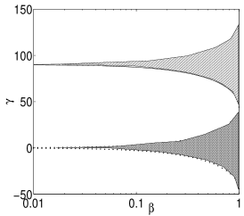
Figure 9: The range of angles between B and v. The dashed area refers to the fast modes, the meshed area represents the range where slow modes fall in. The ranges are produced when the angle between k and B changes from $0$ to $\pi$.

References

- (1) Alfvén, H. & Flthmmar, C.G. 1963, Cosmical Electrodynamics, Oxford, Clarendon Press
- (2) Anderson, N., & Watson, W. D. 1993, A & A, 270, 477
- (3) Armstrong, J. W., Rickett, B. J. & Spangler, S. R. 1995, ApJ, 443, 209
- (4) Arons, J. & Max, C.E. 1975, ApJ, 196, L77
- (5) Biermann, L., & Harwit, M. 1980, ApJ, 241, L105
- (6) Black, J.H., & van Dishoeck, E.F. 1991, ApJ, 369, L9
- (7) Blum, J. 2000, Space Sci. Rev., 92, 265B
- (8) Boldyrev, S., Nordlund, A. & Padoan, P. 2002, ApJ, 573, 678
- (9) Braginskii, S.I. 1965, Rev. Plasma Phys. 1, 205
- (10) Cho, J. & Lazarian, A. 2002, Phys. Rev. Lett., 88, 245001 (CL02)
- (11) Cho, J. & Lazarian, A. 2003a, to appear in Acoustic emission and scattering by turbulent flows, ed. M. Rast (Springer LNP), astro-ph/0301462
- (12) Cho, J. & Lazarian, A. 2003b, Rev. Mex. A&A, Vol. 15, pp. 293 (CL03)
- (13) Cho, J. & Lazarian, A. 2003c, MNRAS, 345, 325
- (14) Cho, J, Lazarian, A., Honein, A., Knaepen B., Kassinos, S. & Moin P. 2003, ApJ, 589, L77
- (15) Cho, J., Lazarian, A. & Vishniac, E.T. 2002a, in “Turbulence and Magnetic field in Astrophys”, eds. T. Passot & E. Falgorone (Springer LNP), p.56
- (16) Cho, J., Lazarian, A. & Vishniac, E.T. 2002b, ApJ, 564, 291 (CLV02)
- (17) Cho, J., Lazarian, A. & Vishniac, E.T. 2002c, ApJL, 566, 49L
- (18) Chokshi, A., Tielens, A.G.G.A. & Hollenbach, D. 1993, ApJ, 407, 806
- (19) Ciolek and Mouschovias 1996, ApJ, 468, 749
- (20) Crutcher, 1999, ApJ, 520, 706
- (21) de Oliveira-Costa, A., Tegmark, M., Devies, R.D., Gutierrez, C.M., Mark J., Haffner, L.M., Jones, A.W., Lasenby, A.N., Rebolo, R., Reynolds, R.J., & Tufte, S.L., Watson, R.A. 2002, ApJ, 567, 363
- (22) Dolginov, A. Z. & Mitrofanov, I. G. 1975, Astronomicheskii Zhurnal, vol. 52, Nov.-Dec. 1975, p. 1268-1278. In Russian.
- (23) Dominik, C. & Tielens, A.G.G.A. 1997, ApJ, 480, 647
- (24) Draine, B.T. 1985, in Protostars and Planets II, ed. D.C. Black & M.S. Matthews (Tucson: Univ. Arizona Press), p.621
- (25) Draine, B. T., & Lazarian, A. 1998, ApJ, 508, 157 (DL98)
- (26) Draine, B. T., Roberge, W. G. & Dalgarno, A. 1983, ApJ, 264, 485
- (27) Draine, B.T., & Salpeter, E.E. 1979, ApJ, 231, 77
- (28) Draine, B.T., & Weingartner, J.C. 1996, ApJ 470, 551
- (29) Ellison, D.C., Drury, L. O’C. & Meyer, J.-P. 1997, ApJ, 487, 197
- (30) Elmegreen, & Fiebig 1993, A&A, 270, 397
- (31) Epstein, R. I. 1980, MNRAS, 193, 723
- (32) Foote, E. A. & Kulsrud, R. M. 1979, ApJ, 233, 302
- (33) Gold, T. 1952, MNRAS, 112, 215
- (34) Goldreich, P. & Sridhar, S. 1995, ApJ, 438, 763
- (35) Greenberg, J. M. & Yencha, A. J. 1973, in IAU Symp 52, p. 369
- (36) Higdon, J. C. 1984, ApJ, 285, 109
- (37) Jokipii, J. R. 1966, ApJ, 146, 480
- (38) Jones, A.P., Tielens, A.G.G.M. & Hollenbach, D.J. 1996, ApJ, 469, 740
- (39) Kim, S. H., Martin, P. G., & Hendry, P. D. 1994, ApJ, 422, 164
- (40) Kulsrud, R. M., & Pearce, W. P., 1969, ApJ, 156, 445
- (41) Kusaka, T., Nakano, T., & Hayashi, C., 1970, Prog. Theor. Phys., 44, 1580
- (42) Hildebrand, R. H., Davidson, J. A., Dotson, J. L., Dowell, C. D., Novak, G. & Vailancourt, J. E. 2000, ASP, 112, 1215
- (43) Lazarian, A. 1994, MNRAS, 268, 713
- (44) Lazarian, A. 1995a, ApJ, 453, 229
- (45) Lazarian, A. 1995b, MNRAS, 274, 679
- (46) Lazarian, A. 1996, in ASP Conf. Proc. 97, Polarimetry of the Interstellar Medium, eds. W. G. Roberge & D. C. B. Whittet (San Francisco: ASP), 425
- (47) Lazarian, A. 1997, ApJ, 483, 296
- (48) Lazarian, A. 1999, Plasma Turbulence and Energetic Particles in Astrophysics, Proceedings of the International Conference, Eds.: Michal Ostrowski, Reinhard Schlickeiser, p. 28
- (49) Lazarian, A. 2000, in “Cosmic Evolution and Galaxy Formation”, ASP, v.215, eds. Jose Franco, Elena Terlevich, Omar Lopez-Cruz, Itziar Aretxaga, p. 69
- (50) Lazarian, A. 2003, Journal of Quantitative Spectroscopy and Radiative Transfer, 79, 881
- (51) Lazarian, A. & Efroimsky, M. 1996, ApJ, 466, 274
- (52) Lazarian, A. & Efroimsky, M. 1999, MNRAS, 303, 673L
- (53) Lazarian, A. & Draine, B.T. 1997, ApJ, 487, 248
- (54) Lazarian, A. & Draine, B.T. 1999a, ApJ, 516, L37
- (55) Lazarian, A. & Draine, B.T. 1999b, ApJ, 520, L67
- (56) Lazarian, A. & Pogosyan, D. 2000, ApJ, 537, 720
- (57) Lazarian, A., Vishniac, E., 1999, ApJ, 517, 700
- (58) Lazarian, A., Vishniac, E. & Cho, J. 2004, ApJ, 603, 180
- (59) Lazarian, A. & Yan, H., 2002a, ApJ, 566, 105L (LY02)
- (60) Lazarian, A. & Yan, H., 2002b, Best of Science, astro-ph/0205283
- (61) Lazarian, A. & Yan, H. 2003, to appear in the proceedings of Astrophysics Dust, astro-ph/0311370
- (62) Lepp, S. 1992, in Astrochemistry of Cosmic Phenomena, IAU Symp. 150, ed. P. Singh (Dordrecht: Kluwer), p. 471
- (63) Lithwick, Y. & Goldreich, P. 2001, ApJ, 562, 279
- (64) Maron, J. & Goldreich, P. 2001, ApJ, 554, 1175
- (65) McCall, B.J., Huneycutt, A.J., Saykally, R.J., Geballe, T.R., Djuric, N., Dunn, G.H., et al. 2003, Nature, 422, 500
- (66) Melrose, D.B. 1980, Plasma Astrophysics (New York: Gordon & Breach).
- (67) Montgomery, D. & Matthaeus, W. 1981, Phys. Fluids, 24 825
- (68) Mukherjee, P., Jones, A.W., Kneissl, R., Lasenby, A.N. 2001, MNRAS, 320, 224
- (69) Nishi, R., Nakano, T., & Umebayashi, T. 1991, ApJ, 368, 181
- (70) Ossenkopf, V. 1993, A&A 280, 617
- (71) Pryadko, J.M. & Petrosian, V. 1997, ApJ, 482, 774
- (72) Purcell, E.M. 1969, Physica 41, 100
- (73) Purcell, E.M. 1979, ApJ, 231, 404
- (74) Ruffle, D.P., Hartquist, T.W., Rawlings, J.M.C., & Williams, D.A. 1998, A&A, 334, 678
- (75) Scalo, J. M. 1987, In Interstellar processes, Proceedings of the Symposium, eds. D.J. Hollenback and Harley A. Thronson, Jr., p. 349
- (76) Schlickeiser, R. & Achatz, U. 1993, J. Plasma Phy. 49, 63
- (77) Schlickeiser, R. & Miller, J. A. 1998, ApJ, 492, 352
- (78) Schlickeiser, R. 2002, Cosmic Ray Astrophysics (Springer-Verlag Berlin Heidelberg)
- (79) Schutte, W. A. & Greenberg, J. M. 1991, A & A 244, 190
- (80) Shebalin, J. V., Matthaeus, W. H., & Montgomery, D. 1983, J. Plasma Phys., 29, 525
- (81) Spitzer, L. & McGlynn, T.A. 1979, ApJ, 231, 417
- (82) Spitzer, L., 1978, Physical Processes in the Interstellar Medium (New York:Wiley)
- (83) Stanimirovic, S. & Lazarian, A. 2001, ApJ, 551, L53
- (84) Völk, H.J., Jones, F.C., Morfill, G.E., & Roser, S. 1980 A&A, 85, 316
- (85) Wakker, B. P. & Mathis, J. S. 2000, ApJ, 544, 107L
- (86) Weidenschilling, S.J. & Ruzmaikina, T.V. 1994, ApJ, 430, 713
- (87) Weingartner, J.C. & Draine, B.T. 2001a, ApJ, 553, 581 (WD01a)
- (88) Weingartner, J.C. & Draine, B.T. 2001b, ApJS, 134, 263 (WD01b)
- (89) Weingartner, J.C., & Draine, B.T. 2002, ApJ, 563, 842
- (90) Welty, D.E., Hobbs, L.M., Lauroesch, J.T., Morton, D.C., Spitzer, L., & York, D.G. 1999, ApJS, 124, 465
- (91) Yan, H. & Lazarian, A. 2002, Phy. Rev. Lett, 89, 281102 (YL02)
- (92) Yan, H. & Lazarian, A. 2003, ApJ, 592, 33L (YL03)
- (93) Yan, H. & Lazarian, A. 2004, accepted to ApJ
- (94) Zank, G.P. & Mattaeus, W.H. 1992, J. Plasma Phys. 48, 85