COSMIC RAY SCATTERING AND STREAMING IN COMPRESSIBLE MAGNETOHYDRODYNAMIC TURBULENCE

Abstract

Recent advances in understanding of magnetohydrodynamic (MHD) turbulence call for revisions in the picture of cosmic ray transport. In this paper we use recently obtained scaling laws for MHD modes to obtain the scattering frequency for cosmic rays. Using quasilinear theory we calculate gyroresonance with MHD modes (Alfvénic, slow and fast) and transit-time damping (TTD) by fast modes. We provide calculations of cosmic ray scattering for various phases of interstellar medium with realistic interstellar turbulence driving that is consistent with the velocity dispersions observed in diffuse gas. We account for the turbulence cutoff arising from both collisional and collisionless damping. We obtain analytical expressions for diffusion coefficients that enter Fokker-Planck equation describing cosmic ray evolution. We obtain the scattering rate and show that fast modes provide the dominant contribution to cosmic ray scattering for the typical interstellar conditions in spite of the fact that fast modes are subjected to damping. We determine how the efficiency of the scattering depends on the characteristics of ionized media, e.g. plasma $\beta$. We calculate the range of energies for which the streaming instability is suppressed by the ambient MHD turbulence.

1 Introduction

Most astrophysical systems, e.g. accretion disks, stellar winds, the interstellar medium (ISM) and intercluster medium are turbulent with an embedded magnetic field that influences almost all of their properties. High conductivity of the astrophysical fluids makes the magnetic fields “frozen in”, and influence fluid motions. The coupled motion of magnetic field and conducting fluid holds the key to many astrophysical processes.

The propagation of cosmic rays (CRs) is affected by their interaction with magnetic field. This field is turbulent and therefore, the resonant interaction of cosmic rays with MHD turbulence has been discussed by many authors as the principal mechanism to scatter and isotropize cosmic rays (Schlickeiser 2002). Although cosmic ray diffusion can happen while cosmic rays follow wandering magnetic fields (Jokipii 1966), the acceleration of cosmic rays requires efficient scattering. For instance, scattering of cosmic rays back into the shock is a vital component of the first order Fermi acceleration (see Longair 1997).

While most investigations are restricted to Alfvén modes propagating along an external magnetic field (the so-called slab model of Alfvénic turbulence), obliquely propagating MHD modes have been included in Fisk et al. (1974) and later studies ( Pryadko & Petrosian 1999). A more complex models were obtained by combining the results of the Reduced MHD with parallel slab-like modes have been also considered (Bieber et al. 1988). Here we attempt to use models that are motivated by the recent studies of MHD turbulence (Goldreich& Sridhar 1995, see Cho, Lazarian & Yan 2002 for a review and references therein).

A recent study (Lerche & Schlickeiser 2001) found a strong dependence of scattering on turbulence anisotropy. Therefore the calculations of CR scattering must be done using a realistic MHD turbulence model. An important attempt in this direction was carried out in Chandran (2000). However, only incompressible motions were considered. On the contrary, ISM is highly compressible. Compressible MHD turbulence has been studied recently (see review by Cho & Lazarian 2003a and references therein). Schlickeiser & Miller (1998) addressed the scattering by fast modes. But they did not consider the damping, which is essential for fast modes. In this paper we discuss in detail various damping processes which can affect the fast modes. To characterize the turbulence we use the statistics of Alfvénic modes obtained in Cho, Lazarian & Vishniac (2002, henceforth CLV02) and compressible modes obtained in Cho & Lazarian (2002, henceforth CL02, 2003b, henceforth CL03).

As MHD turbulence is an extremely complex process, all theoretical constructions should be tested thoroughly. Until very recently matching of observations with theoretical constructions used to be the only way of testing. Indeed, it is very dangerous to do MHD turbulence testing without fully 3D MHD simulations with a distinct inertial range. Theoretical advances related to the anisotropy of MHD turbulence and its scalings (see Shebalin et al. 1983, Higdon 1984, Montgomery, Brawn & Matthaeus 1987, Shebalin & Montgomery 1988, Zank & Matthaeus 1992) were mostly done in relation with the observations of fluctuations in outer heliosphere and solar wind. Computers allowed an alternative important way of dealing with the problem. While still presenting a limited inertial range, they allow to control the input parameters well making it easier to test theoretical ideas. For instance, one of us involved in the compressible turbulence research, failed so far to observe in the simulations the characteristic features, e.g. the production of a substantial amount of the quasi-parallel modes that are predicted by some of earlier MHD turbulence theories and were used to justify the slab geometry approximation for cosmic ray scattering. In this respect, the observational evidence in favor of such modes could be interpreted as the result of angle-dependent damping that we touch upon in this paper.

While actual MHD turbulence is and will be in the near future the subject of intensive research and scientific disputes, in the present paper we adopt a simple model of turbulence that seems to be consistent with present day numerical MHD simulations.

Yan & Lazarian (2002, henceforth YL02) used recent advances in understanding of MHD turbulence (CL02) to describe cosmic ray propagation in the galactic halo. In this paper we undertake a detailed study of cosmic ray scattering rates in different idealized phases of the interstellar medium. In $\S$2, we describe our model of turbulence, introduce the statistics of Alfvénic and compressible turbulence in various conditions, including both high $\beta$ and low $\beta$ cases. In $\S$3, we describe the resonant interactions between the MHD modes and CRs. The scattering by Alfvén modes and fast modes is presented in $\S$4. We apply our results to different phases of ISM, including Galactic halo, warm ionized medium (WIM), hot ionized medium (HIM), and also partially ionized medium. In $\S$5, we describe the streaming instability in the presence of background turbulence. Discussion of our results is provided in $\S$6 while the summary is given in $\S$7.

2 MHD cascade and its damping

2.1 Adopted model of MHD turbulence cascade

A shortcoming of many earlier studies was that the crucial element for cosmic ray scattering, namely, MHD turbulence briefly describe the model of turbulent cascade adopted and refer the reader to the original papers for a detailed explanation.

Understanding of the properties of MHD turbulence is a challenging problem dealt with by many researchers. This work is not the appropriate place to cite all the important papers that shaped the field. For instance, a very incomplete list of such references in a review by Cho, Lazarian & Vishniac (2003) contains more than a hundred entries.

It is well known that linear MHD perturbations can be decomposed into Alfvénic, slow and fast waves with well-defined dispersion relations (see Alfvén & Fälthammar 1963). Important questions arise. Can the MHD perturbations that characterize turbulence be separated into distinct modes? Can the linear modes be used for this purpose? Is it possible to talk about, for instance, an Alfvénic cascade in a compressible medium? The answer to these non trivial questions is critical to studying cosmic ray scattering.

The separation into Alfvén and pseudo-Alfvén modes, which are the incompressible limit of Alfvén modes, is an essential element of the Goldreich-Sridhar (1995, henceforth GS95) model of turbulence. The arguments there were provided in favor of Alfvén modes developing a cascade on their own, while the pseudo-Alfvén modes would passively follow the cascade. The drain of Alfvénic mode energy to pseudo-Alfvén modes was shown to be marginal along the cascade.

This model and the legitimacy of the separation into modes were tested successfully with incompressible MHD numerical simulations (Cho & Vishniac 2000; Maron & Goldreich 2001, CLV02). This motivated a further study of the issue within the compressible medium.

The separation of MHD perturbations in compressible media into different modes was discussed further in Lithwick & Goldreich 2001 and CL02. There arguments were provided why one does not expect the modes to get entangled into an inseparable mess even in spite of the fact that MHD turbulence is a highly non-linear phenomenon.

The actual decomposition of MHD turbulence into Alfvén, slow and fast modes was a challenge that was addressed in CL02, CL03. There a particular realization of turbulence with mean magnetic field comparable to the fluctuating magnetic field was studied. This setting is probably typical of the Galactic magnetic field and would allow us to use a statistical procedure of decomposition in the Fourier space, where the basis of the Alfvén, slow and fast perturbations was defined. For some particular cases, e. g. for the case of low $\beta$ medium, the procedure was benchmarked successfully and therefore argued to be reliable (see CL03 for more details).

We also want to stress that the numerical studies in CL02 and CL03 were not blind empirical studies. They were aimed to test theoretical expectations. The very fact that for all the tested cases the theory was confirmed, makes us confident about the theory.

Unlike hydrodynamic turbulence, Alfvénic one is anisotropic, with eddies elongated along the magnetic field (see Higdon 1984, Shebalin et al 1983). On the intuitive level it can be explained as the result of the following fact: it is easier to mix the magnetic field lines perpendicular to the direction of the magnetic field rather than to bend them. However, one cannot do mixing in the perpendicular direction to very small scales without affecting the parallel scales. This is probably the major difference between the adopted model of Alfvénic perturbations and the Reduced MHD (see Bieber et al. 1994). In the GS95 model as well as in its generalizations for compressible medium mixing motions induce the reductions of the scales of the parallel perturbations.

The corresponding scaling can be easily obtained. For instance, calculations in CLV02 prove that motions perpendicular to magnetic field lines are essentially hydrodynamic. As the result, energy transfer rate due to those motions is constant $\dot{E_{k}}\sim v_{k}^{2}/\tau_{k}$, where $\tau_{k}$ is the energy eddy turnover time $\sim(v_{k}k_{\perp})^{-1}$, where $k_{\perp}$ is the perpendicular component of the wave vector $\mathbf{k}$. The mixing motions couple to the wave-like motions parallel to magnetic field giving a critical balance condition, i.e., $k_{\bot}v_{k}\sim k_{\parallel}V_{A}$, where $k_{\parallel}$ is the parallel component of the wave vector $\mathbf{k}$, $V_{A}$ is the Alfvén speed. From these arguments, the scale dependent anisotropy $k_{\parallel}\propto k_{\perp}^{2/3}$and a Kolmogorov-like spectrum for the perpendicular motions $v_{k}\propto k^{-1/3}$ can be obtained (see Lazarian & Vishniac 1999).

It was conjectured in Lithwick & Goldreich (2001) that GS95 scaling should be approximately true for Alfvén and slow modes in moderately compressible plasma. For magnetically dominated, the so-called low $\beta$ plasma, CL02 showed that the coupling of Alfvénic and compressible modes is weak and that the Alfvénic and slow modes follow the GS95 spectrum. This is consistent with the analysis of HI velocity statistics (Lazarian & Pogosyan 2000, Stanimirovic & Lazarian 2001) as well as with the electron density statistics (see Armstrong, Rickett & Spangler 1995). Calculations in CL03 demonstrated that fast modes are marginally affected by Alfvén modes and follow acoustic cascade in both high and low $\beta$ medium. In what follows, we consider both Alfvén modes and compressible modes and use the description of those modes obtained in CL02, CL03 to study CR scattering by MHD turbulence.

The distribution of energy between compressible and incompressible modes depends, in general, on the way turbulence is driven. Both the scale of driving and how the driving is performed matter. CL02 and CL03 studied generation of compressible perturbations using random incompressible driving with the energy coming from the largest scales of the system. While in the interstellar medium the energy can be injected at different scales, the bulk of the injected energy comes from the large scales (see Mac Low 2002) which explains the power spectra of turbulence observed (see discussion in Lazarian & Cho 2003). If the injection of energy happens at velocity higher that the Alfvén velocity up to the scale at which $V_{l}\approx V_{A}$ the turbulence has hydrodynamic character. At smaller scales Alfvénic, fast and slow modes cascades develop. At the large scale the turbulence is isotropic in this case for all modes. The opposite case of injection velocity less than $V_{A}$ results in the Alfvén and slow cascade being anisotropic even at the injection scale, provided that the driving is isotropic.

How much energy is injected into fast modes if the driving takes place at large scales? If energy is initially injected in terms of Alfvénic perturbation, then the energy in fast $\sim\delta V_{f}^{2}$ and Alfvén $\sim\delta V_{A}^{2}$ modes are related by (CL02),

$$(\delta V_{f}/\delta V_{A})^{2}\sim\delta V_{A}\times V_{A}/(V_{A}^{2}+C_{S}^{2}),$$ (1)

where $C_{S}$ is the sound speed. This relation testifies that at large scales incompressible driving can transfer an appreciable part of energy into fast modes. However, at smaller scales the drain of energy from Alfvén to fast modes is marginal. Therefore the cascades evolve without much of cross talk. In high $\beta$ medium, however, the velocity perturbation $\delta V$ at injection scale may be larger than Alfvén speed. The injection speed of fast modes in this case can be approximated as $\delta V_{f}/\delta V\sim(\delta V/C_{S})^{2}$. Naturally a more systematic study of different types of driving is required. In the absence of this, in what follows we assume that equal amounts of energy are transfered into fast and Alfvén modes when driving is at large scales.

2.2 Plasma effects and damping of turbulence

In many earlier papers Alfvénic turbulence was considered by many authors as the default model of interstellar magnetic turbulence. This was partially motivated by the fact that unlike compressible modes, the Alfvén ones are essentially free of damping in fully ionized medium (see Ginzburg 1961, Kulsrud & Pearce 1969). In the paper below we will show that compressible fast modes are particularly important for cosmic ray scattering. For them damping is essential.

At small scales turbulence spectrum is altered by damping. Various processes can damp the MHD motions (see Appendix A for details). In partially ionized plasma, the ion-neutral collisions are the dominant damping process. In fully ionized plasma, there are basically two kinds of damping: collisional or collisionless damping. Their relative importance depends on the mean free path in the medium (Braginskii 1965),

$$l_{mfp}=v_{th}\tau=6\times 10^{11}{\rm cm}(T/8000{\rm K})^{2}/(n/{\rm cm}^{-3}).$$ (2)

If the wavelength is larger than the mean free path, viscous damping dominates. If, on the other hand, the wavelength is smaller than mean free path, then the plasma is in the collisionless regime and collisionless damping is dominant.

To obtain the truncation scale, the damping time $\Gamma_{d}^{-1}$ should be compared to the cascading time $\tau_{k}$. As we mentioned earlier, the Alfvénic turbulence cascades over one eddy turn over time $(k_{\perp}v_{k})^{-1}\sim(k_{\parallel}V_{A})^{-1}$. The cascade of fast modes takes a bit longer:

$$\tau_{k}=\omega/k^{2}v_{k}^{2}=(k/L)^{-1/2}\times V_{ph}/V^{2},$$ (3)

where $V$ is the turbulence velocity at the injection scale, $V_{ph}$ is is the phase speed of fast modes and equal to Alfvén and sound velocity for high and low $\beta$ plasma, respectively (CL02). If the damping is faster than the turbulence cascade, the turbulence gets truncated. Otherwise, for the sake of simplicity, we ignore the damping and assume that the turbulence cascade is unaffected. As the transfer of energy between Alfvén, slow and fast modes of MHD turbulence is suppressed at the scales less than the injection scale, we consider different components of MHD cascade independently.

We get the cutoff scale $k_{c}$ by equating the damping rate and cascading rate $\tau_{k}\Gamma_{d}\simeq 1$. Then we check whether it is self-consistent by comparing the $k_{c}$ with the relevant scales, e.g., injection scale, mean free path and the ion gyro-scale.

Damping is, in general, anisotropic, i.e., the linear damping (see Appendix A) depends on the angle $\theta$ between the wave vector ${\bf k}$ and local direction of magnetic field ${\bf B}$. Unless randomization of $\theta$ is comparable to the cascading rate the damping scale gets angle-dependent. The angle $\theta$ varies because of both the randomization of wave vector $\bf k$ and the wandering of magnetic field lines. Consider fast modes, that will be shown to be the most important for cosmic ray scattering. Their non-linear cascading can be characterized by interacting wave vectors ${\bf k}$ that are nearly collinear (see review by Cho, Lazarian & Vishniac 2003). The possible transversal deviation $\delta k$ can be estimated from the uncertainty condition $\delta\omega t_{cas}\sim 1$, where $\delta\omega\sim V_{ph}\delta k(\delta k/k)$. Combining with Eq.(3), we can get

$$\delta k/k\simeq\frac{1}{(kL)^{1/4}}\left(\frac{V}{V_{ph}}\right)^{1/2}.$$ (4)

The field line wandering is mainly caused by shearing via Alfvén modes. The deviation of field lines during one cascading period of fast modes can be estimated as:

$$\frac{\delta B}{B}\simeq\left(\frac{V}{L}\right)^{1/2}\tau_{k}^{1/2}=\frac{1}{(kL)^{1/4}}\left(\frac{V_{ph}}{V}\right)^{1/2}.$$ (5)

Thus the variation of the angle between ${\bf k}$ and $\bf B$ $\delta\theta\sim(1/kL)^{1/4}$ is marginal at large $k$. In the presence of anisotropic damping this results in anisotropic distribution of fast mode energy at large $k$.

With this input at hand, it is possible to determine the turbulence damping scales for a given medium. For waves in fully ionized medium one should compare the wavelength and mean free path before determining which damping should be applied. However, when we deal with the turbulence cascade the situation is more complicated: If the mean free path is larger than the turbulence injection scale, we can simply apply the collisionless damping to the whole inertial range of turbulence. In general one should compare the viscous cut off and the mean free path. If the cutoff scale is larger than the mean free path, it shows that the turbulence is indeed cut off by the viscous damping. Otherwise, we neglect the viscous damping and just apply the collisionless damping to the turbulence below the mean free path. By comparing different damping, we find the dominant damping processes for the idealized ISM phases (see Table1).

ISM	galactic halo	HIM	WIM	WNM	CNM	DC
T(K)	$2\times 10^{6}$	$1\times 10^{6}$	8000	6000	100	15
$C_{S}$(km/s)	130	91	8.1	7	0.91	0.35
n(cm-3)	$10^{-3}$	$4\times 10^{-3}$	0.1	0.4	30	200
$l_{mfp}$(cm)	$4\times 10^{19}$	$2\times 10^{18}$	$6\times 10^{12}$	$8\times 10^{11}$	$3\times 10^{6}$	$10^{4}$
L(pc)	100	100	50	50	50	50
B($\mu$G)	5	2	5	5	5	15
$\beta$	0.28	3.5	0.11	0.33	0.42	0.046
damping	collisionless	collisional	collisional	neutral-ion	neutral-ion	neutral-ion

Table 1: The parameters of idealized ISM phases and relevant damping. The dominant damping mechanism for turbulence is given in the last line. HIM=hot ionized medium, CNM=cold neutral medium, WNM=warm neutral medium, WIM=warm ionized medium, DC=dark cloud.

2.3 Statistics of fluctuations

Within random-phase approximation, the correlation tensor in Fourier space is (see Schlickeiser & Achatz 1993)

$$<B_{i}(\mathbf{k})B_{j}^{*}(\mathbf{k^{\prime}})>/B_{0}^{2}=\delta(\mathbf{k}-\mathbf{k^{\prime}})M_{ij}(\mathbf{k}),$$

$$<v_{i}(\mathbf{k})B_{j}^{*}(\mathbf{k^{\prime}})>/V_{A}B_{0}=\delta(\mathbf{k}-\mathbf{k^{\prime}})C_{ij}(\mathbf{k}),$$

$$<v_{i}(\mathbf{k})v_{j}^{*}(\mathbf{k^{\prime}})>/V_{A}^{2}=\delta(\mathbf{k}-\mathbf{k^{\prime}})K_{ij}(\mathbf{k}),$$ (6)

where $B_{i}$, $v_{i}$ are respectively the magnetic and velocity perturbation associated with the turbulence. For the balanced cascade we consider, i.e., equal intensity of forward and backward modes, $C_{ij}(\mathbf{k})=0$.

The isotropic tensor usually used in the literature is

$$M_{ij}(\mathbf{k})=C_{0}\{\delta_{ij}-k_{i}k_{j}/k^{2}\}k^{-11/3},$$ (7)

The normalization constant $C_{0}$ here can be obtained if the energy input at the scale $L$ is defined. Assuming equipartition $u_{k}=\int dk^{3}\sum_{i=1}^{3}M_{ii}B_{0}^{2}/8\pi\sim B_{0}^{2}/8\pi$, we get $C_{0}=L^{-2/3}/12\pi$. The normalization for the tensors below are obtained in the same way.

The analytical fit to the anisotropic tensor for Alfvén modes, obtained in CLV02 is,

$$\left[\begin{array}[]{c}M_{ij}({\mathbf{k}})\\ K_{ij}({\mathbf{k}})\end{array}\right]=\frac{L^{-1/3}}{6\pi}I_{ij}k_{\perp}^{-10/3}\exp(-L^{1/3}|k_{\parallel}|/k_{\perp}^{2/3}),$$ (8)

where $I_{ij}=\{\delta_{ij}-k_{i}k_{j}/k^{2}\}$ is a 2D tensor in $x-y$ plane which is perpendicular to the magnetic field, $L$ is the injection scale, $V$ is the velocity at the injection scale. Slow modes are passive and similar to Alfvén modes.

According to CL02, fast modes are isotropic and have one dimensional energy spectrum $E(k)\propto k^{-3/2}$. In low $\beta$ medium, the corresponding correlation is (YL02)

$$\left[\begin{array}[]{c}M_{ij}({\mathbf{k}})\\ K_{ij}({\mathbf{k}})\end{array}\right]={\frac{L^{-1/2}}{8\pi}}H_{ij}k^{-7/2}\left[\begin{array}[]{c}\cos^{2}\theta\\ 1\end{array}\right],$$ (9)

where $\theta$ is the angle between $\mathbf{k}$ and $\mathbf{B}$, $H_{ij}=k_{i}k_{j}/k_{\perp}^{2}$ is also a 2D tensor in $x-y$ plane. The factor $\cos^{2}\theta$ represents the projection as magnetic perturbations are perpendicular to $\mathbf{k}$.

In high $\beta$ medium, fast modes in this regime are essentially sound modes compressing magnetic field (GS95, Lithwick & Goldreich 2001, CL03). The compression of magnetic field depends on plasma $\beta$. The corresponding x-y components of the tensors are

$$\left[\begin{array}[]{c}M_{ij}({\mathbf{k}})\\ K_{ij}({\mathbf{k}})\end{array}\right]={\frac{L^{-1/2}}{2\pi}}\sin^{2}\theta H_{ij}k^{-7/2}\left[\begin{array}[]{c}\cos^{2}\theta/\beta\\ 1\end{array}\right].$$ (10)

The velocity perturbations in high $\beta$ medium are radial, i.e., along $\mathbf{k}$, thus we have the factor $\sin^{2}\theta$ and also $V_{A}^{2}/C_{s}^{2}=2/\beta$ from the magnetic field being frozen $\omega\delta\mathbf{B}\sim\mathbf{k}\times(\mathbf{v}_{k}\times\mathbf{B})$. We use these statistics to calculate cosmic ray scattering arising from MHD turbulence.

3 Interactions between turbulence and particles

Basically there are two types of resonant interactions: gyroresonance acceleration and transit acceleration (henceforth TTD). The resonant condition is $\omega-k_{\parallel}v\mu=n\Omega$ ($n=0,\pm 1,2...$), where $\omega$ is the wave frequency, $\Omega=\Omega_{0}/\gamma$ is the gyrofrequency of relativistic particle, $\mu=\cos\xi$, where $\xi$ is the pitch angle of particles. TTD formally corresponds to $n=0$ and it requires compressible perturbations.

We employ quasi-linear theory (QLT) to obtain our estimates. If mean magnetic field is larger than the fluctuations at the injection scale, we may say that the QLT treatment we employ defines parallel diffusion. Obtained by applying the QLT to the collisionless Boltzmann-Vlasov equation, the Fokker-Planck equation is generally used to describe the evolvement of the gyrophase-averaged distribution function $f$,

$$\frac{\partial f}{\partial t}=\frac{\partial}{\partial\mu}\left(D_{\mu\mu}\frac{\partial f}{\partial\mu}+D_{\mu p}\frac{\partial f}{\partial p}\right)+\frac{1}{p^{2}}\frac{\partial}{\partial p}\left[p^{2}\left(D_{\mu p}\frac{\partial f}{\partial\mu}+D_{pp}\frac{\partial f}{\partial p}\right)\right],$$

where $p$ is the particle momentum. The Fokker-Planck coefficients $D_{\mu\mu},D_{\mu p},D_{pp}$ are the fundamental physical parameter for measuring the stochastic interactions, which are determined by the electromagnetic fluctuations (Schlickeiser & Achatz1993):

Adopting the approach in (Schlickeiser & Achatz 1993) and taking into account only the dominant interaction at $n=\pm 1$, we can get the Fokker-Planck coefficients (see Appendix B),

$$\left(\begin{array}[]{c}D_{\mu\mu}\\ D_{pp}\end{array}\right)={\frac{\pi\Omega^{2}(1-\mu^{2})}{2}}\int_{\bf k_{min}}^{\bf k_{max}}dk^{3}\delta(k_{\parallel}v_{\parallel}-\omega\pm\Omega)$$ (13)

$$\left(\begin{array}[]{c}\left(1+\frac{\mu V_{ph}}{v\zeta}\right)^{2}\\ m^{2}V_{A}^{2}\end{array}\right)\left\{(J_{2}^{2}({\frac{k_{\perp}v_{\perp}}{\Omega}})+J_{0}^{2}({\frac{k_{\perp}v_{\perp}}{\Omega}}))\right.$$ (16)

$$\left[\begin{array}[]{c}M_{{\mathcal{RR}}}({\mathbf{k}})+M_{{\mathcal{LL}}}({\mathbf{k}})\\ K_{{\mathcal{RR}}}({\mathbf{k}})+K_{{\mathcal{LL}}}({\mathbf{k}})\end{array}\right]-2J_{2}({\frac{k_{\perp}v_{\perp}}{\Omega}})J_{0}({\frac{k_{\perp}v_{\perp}}{\Omega}})$$ (19)

$$\left.\left[e^{i2\phi}\left[\begin{array}[]{c}M_{{\mathcal{RL}}}({\mathbf{k}})\\ K_{{\mathcal{RL}}}({\mathbf{k}})\end{array}\right]+e^{-i2\phi}\left[\begin{array}[]{c}M_{{\mathcal{LR}}}({\mathbf{k}})\\ K_{{\mathcal{LR}}}({\mathbf{k}})\end{array}\right]\right]\right\},$$ (24)

where $\zeta=1$ for Alfvén modes and $\zeta=k_{\parallel}/k$ for fast modes, $k_{min}=L^{-1}$, $k_{max}=\Omega_{0}/v_{th}$ corresponds to the dissipation scale, $m=\gamma m_{H}$ is the relativistic mass of the proton, $v_{\perp}$ is the particle’s velocity component perpendicular to $\mathbf{B}_{0}$, $\phi=\arctan(k_{y}/k_{x}),$ ${\mathcal{L}},{\mathcal{R}}=(x\pm iy)/\sqrt{2}$ represent left and right hand polarization.

The delta function $\delta(k_{\parallel}v_{\parallel}-\omega+n\Omega)$ approximation to real interaction is true when magnetic perturbations can be considered static (Schlickeiser 1993). For cosmic rays, $k_{\parallel}v_{\parallel}\gg\omega$ so that the resonant condition is essentially $k_{\parallel}v\mu-n\Omega=0$. From this resonance condition, we know that the most important interaction occurs at $k_{\parallel}=k_{\parallel,res}=\Omega/v_{\parallel}$. This is generally true except for small $\mu$ (or scattering near $90^{o}$).

4 Scattering of cosmic rays

4.1 Scattering by Alfvénic turbulence

As we discussed in $\S$2, Alfvén modes are anisotropic, eddies are elongated along the magnetic field, i.e., $k_{\perp}>k_{\parallel}$. The scattering of CRs by Alfvén modes is suppressed first because most turbulent energy goes to $k_{\perp}$ due to the anisotropy of the Alfvénic turbulence so that there is much less energy left in the resonance point $k_{\parallel,res}=\Omega/v_{\parallel}\sim r_{L}^{-1}$. Furthermore, $k_{\perp}\gg k_{\parallel}$ means $k_{\perp}\gg r_{L}^{-1}$ so that cosmic ray particles have to be interacting with lots of eddies in one gyro period. This random walk substantially decreases the scattering efficiency. The scattering by Alfvén modes was studied in YL02, (see Appendix B). In case that the pitch angle $\xi$ not close to 0, the analytical result is

$$\left[\begin{array}[]{c}D_{\mu\mu}\\ D_{pp}\end{array}\right]=\frac{v^{2.5}\mu^{5.5}}{\Omega^{1.5}L^{2.5}(1-\mu^{2})^{0}.5}\Gamma[6.5,k_{max}^{-\frac{2}{3}}k_{\parallel,res}L^{\frac{1}{3}}]\left[\begin{array}[]{c}1\\ m^{2}V_{A}^{2}\end{array}\right],$$ (25)

where $\Gamma[a,z]$ is the incomplete gamma function. The presence of this gamma function in our solution makes our results orders of magnitude larger than those in Chandran (2000) for the most of energies considered. However, the scattering frequency,

$$\nu=2D_{\mu\mu}/(1-\mu^{2}),$$ (26)

are still much smaller than the estimates for isotropic and slab model (see YL02). As the anisotropy of the Alfvén modes is increasing with the decrease of scales, the interaction with Alfvén modes becomes more efficient for higher energy cosmic rays. When the Larmor radius of the particle becomes comparable to the injection scale, which is likely to be true in the shock region as well as for very high energy cosmic rays in diffuse ISM, Alfvén modes get important.

It’s worthwhile to mention the imbalanced cascade of Alfvén modes (CLV02). Our basic assumption above was that Alfvén modes were balanced, meaning that the energy of modes propagating one way was equal to that in opposite direction. In reality, many turbulence sources are localized so that the modes leaving the sources are more energetic than those coming toward the sources. The energy transfer in the imbalanced cascade occurs at a slower rate, and the Alfvén modes behave more like waves. The scattering by these imbalanced Alfvén modes could be more efficient. However, as the actual degree of anisotropy of imbalanced cascade is currently uncertain, and the process will be discussed elsewhere.

4.2 Scattering by fast modes

The contribution from slow modes is no more than that by Alfvén modes since the slow modes have the similar anisotropies and scalings. More promising are fast modes, which are isotropic (CL02). With fast modes there can be both gyroresonance and transit-time damping (TTD) (Schlickeiser & Miller 1998).

TTD happens due to the resonant interaction with parallel magnetic mirror force. The advantage of TTD is that it doesn’t have a distinct resonant scale associated with it. TTD is thus an alternative to scattering of low energy CRs which Larmor radii are below the damping scale of the fast modes. Moreover, we shall show later that TTD can contribute substantially to cosmic ray acceleration (also known as the second order Fermi acceleration). This can be crucial in some circumstances, e.g., for $\gamma$ ray burst (Lazarian et al. 2003), and acceleration of charged particles (Yan & Lazarian 2003). Different from gyroresonance, the resonance function of TTD is broadened even for CRs with small pitch angles. The formal resonance peak $k_{\parallel}/k=V_{ph}/v_{\parallel}$ favors quasi-perpendicular modes. However, these quasi-perpendicular modes cannot form an effective mirror to confine CRs because the gradient of magnetic perturbations along the mean field direction $\nabla_{\parallel}\mathbf{B}$ is small. Thus the resonance peak is weighted out and the Breit-Wigner-type resonance function should be adopted (see eq.B49 and Schlickeiser & Achatz 1993).

Here we apply our analysis to the various phases of ISM.

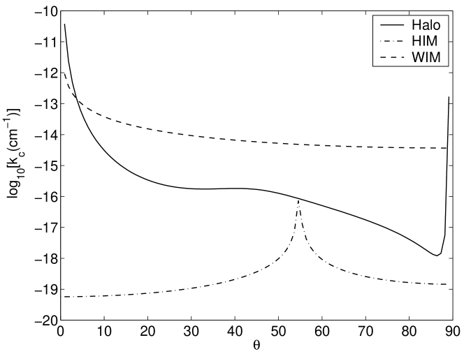
Figure 1: Damping scale vs. the angle $\theta$ between ${\bf k}$ and $\bf B$ in halo, HIM and WIM.

Halo

Recent observations (Beck 2001) suggest that the galactic halos are magnetically dominant, corresponding to low $\beta$ medium. For low $\beta$ medium, we use the tensors given by Eq.(9). For the halo, since damping at the scale of mean free path is slower than cascading, fast modes cascade further to collisionless regime and are subjected to collisionless damping. As we see from Eq.(A2), the damping increases with $\theta$ unless $\theta$ is close to $\pi/2$. This means that those fast modes in the two narrow cones with axis parallel and perpendicular to the magnetic field are less damped. For those quasi-parallel modes the argument for the Bessel function in Eq.(B20) is $k_{\perp}\tan\xi/k_{\parallel,res}<1$ unless $\xi$ is close to $90^{o}$. So we can take advantage of the anisotropy of the damped fast modes and use the asymptotic form of Bessel function for small argument $J_{n}(x)\simeq(x/2)^{n}/n!$ to obtain the corresponding analytical result for this case (see Appendix B):

$$\left[\begin{array}[]{c}D_{\mu\mu}\\ D_{pp}\end{array}\right]=\frac{\pi(\Omega v\mu)^{0.5}(1-\mu^{2})}{2L^{0.5}}$$ (29)

$$\left[\begin{array}[]{c}(1-(\left(\frac{k_{\perp,c}}{k_{\parallel,res}}\right)^{2}+1)^{-\frac{7}{4}})/7\\ (1-(\left(\frac{k_{\perp,c}}{k_{\parallel,res}}\right)^{2}+1)^{-\frac{3}{4}})m^{2}V_{A}^{2}/3\end{array}\right]$$ (32)

The contribution from those quasi-perpendicular modes is

$$\left[\begin{array}[]{c}\Delta D_{\mu\mu}\\ \Delta D_{pp}\end{array}\right]\simeq\frac{\pi(\Omega v\mu(1-\mu^{2}))^{0.5}}{3L^{0.5}}$$ (35)

$$\left[\begin{array}[]{c}\left(\frac{k_{\parallel,res}}{k^{\prime}_{\perp,c}}\right)^{4.5}/4.5\\ \left(\frac{k_{\parallel,res}}{k^{\prime}_{\perp,c}}\right)^{2.5}m^{2}V_{A}^{2}/2.5\end{array}\right].$$ (38)

As we can see in Fig.1, the quasi-perpendicular modes are confined in a much narrower cone than quasi-parallel modes, which indicates that $\frac{k_{\perp,c}}{k_{\parallel,res}}\gg\frac{k_{\parallel,res}}{k^{\prime}_{\perp,c}}$. Thus $\Delta D_{\mu\mu}\ll D_{\mu\mu}$. This is understandable because quasi-perpendicular modes have the similar anisotropy as Alfvén modes, which has been shown negligible for CR scattering.

From Eq.(32), we see the key factor is $(k_{\perp,c}/k_{\parallel,res})=\tan\theta_{c}$. Using Eq.(A2) and the relation $\tau_{k}\Gamma_{L}\simeq 1$, we see the critical angle $\theta_{c}$ decreases with the energy of CRs $\tan\theta_{c}>2(m_{i}/\pi m_{e}\beta kL)^{1/4}\propto r_{L}^{1/4}$. Therefore scattering frequency in the halo increases slowly with energy. Since the variation of $\theta$ during cascade $\delta\theta\simeq 1/(kL)^{1/4}\ll\theta_{c}$ at the corresponding scales, we assume the only effect of this variation is to reduce $\theta_{c}$ by $\delta\theta$. Fig.2a. shows the result corresponding to a pitch angle $\xi=45^{o}$ and we will adopt this value for the following calculations. The contribution from TTD can be obtained by evaluating Eq.(B49) numerically. The contribution is mostly from quasi-perpendicular propagating modes for which the collisionless damping is minimal (see Eq.A2). Limited by the variation of $\theta$, the smallest scale the cascade can reach is a scale corresponding to $k_{c}(\pi/2-\delta\theta)$. Combining with Eq.(4) and (5), we can solve Eq.(A2) iteratively and get $k_{c}(\pi/2-\delta\theta)\simeq 4.3\times 10^{-14}\rm cm^{-1}$. The contribution of TTD to scattering is smaller than that of gyroresonance (see Fig.2a and 3a) except for small $\mu$.

WIM

According to the results in $\S$2, the warm ionized medium (WIM) is also in low $\beta$ but collisional regime. The mean free path $l_{mfp}=6\times 10^{12}$cm (table1), which corresponds to the resonant scale of CRs with energy $\sim 10$GeV. Thus For CRs harder than 10GeV the resonant modes with $k_{\parallel}=\Omega/v_{\parallel}$ are subjected to collisional damping. Since the viscous damping increases with $\theta$, we can apply Eq.(32) to the gyroresonance in WIM as well. By equating the damping rate Eq.(A4) with the cascading rate Eq.(3), we can obtain $\tan\theta_{c}>V_{A}/(k^{3/4}l^{1/4})\sqrt{6\rho_{i}/\eta_{0})}\propto r_{L}^{3/4}$. Thus according to Eq.(32) the scattering frequency curve in WIM gets steeper (see Fig.2b). The angle variation $\delta\theta\simeq 1/(kL)^{1/4}<\theta_{c}$ for CRs $>10$GeV, so we adopt the same treatment as above, namely, subtracting $\delta\theta$ from $\theta_{c}$. For lower energy CRs, the only available modes are those with ${\bf k}$ in a small cone as the residual of the collisional damping at large scales. Certainly, these modes are also affected by collisionless damping. However, the pitch angle of these modes is so small that the collisionless process is marginal. For scattering of CRs with low energy or large pitch angles, TTD is an alternative and can be evaluated by Eq.(B49) (see Fig.2b & 3b).

Hot Ionized Medium

Hot ionized medium (HIM) is in high $\beta$ regime and we adopt the tensors given by Eq.(10). The mean free path of the HIM is of the order of parsec and thus the fast modes in this medium are subjected to collisional damping (see table1). We use Eq.(A4) to acquire the formal damping scale as a function of $\theta$. As shown in Fig.1), the peak around $\theta\sim 53^{o}$ indicates that damping is the weakest here. However, since the angle variation $\delta\theta\sim 1/(kL)^{1/4}\sim 20^{o}$ is large at the scale of mean free path $2\times 10^{18}$cm, the cascade doesn’t get though mean free path. Therefore, there is no gyroresonance interaction for moderate energy CRs. The only available interaction is TTD. The scattering frequency is $\sim 1.2\times 10^{-13}\rm s^{-1}$ for the energy range considered.

Partially ionized media

Partially ionized media are similar to HIM in the sense that fast modes are severely damped by the ion-neutral damping. The cascade is cut off before the resonant scales of most of the CRs we consider. Indeed, for the parameters chosen, we find that gyroresonance only contribute to the transport of CRs of energy $\geq 0.8$TeV in DC and $>1$TeV for WNM and CNM. Therefore only TTD contributes to the scattering of moderate energy CRs in these media. As expected, the scattering is less efficient in partially ionized media. The scattering frequencies for moderate energy CRs are $2.5\times 10^{-14}\rm s^{-1}$ in WNM, $\sim 4.0\times 10^{-15}\rm s^{-1}$ in CNM and $5.7\times 10^{-15}\rm s^{-1}$ in MC.

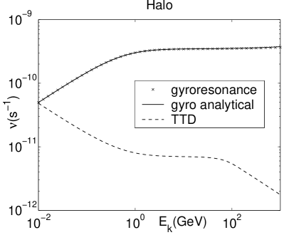
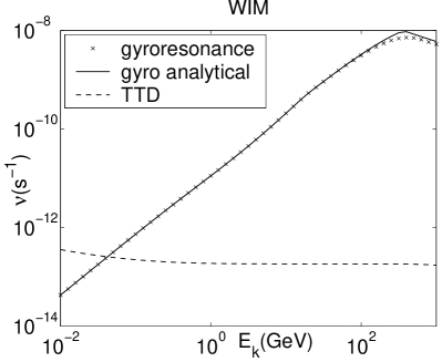
Figure 2: Scattering frequency $\nu$ given by Eq.(26) vs. the kinetic energy $E_{k}$ of cosmic rays (a) in halo, (b) in WIM. The ’x’ lines refer to scattering by gyroresonance and solid lines are the corresponding analytical results given by Eq.(32). The dashed line are the results from Eq.(B49) for TTD.

From the above results, we see that the fast modes dominate CRs’ scattering in spite of the damping. From Eq.(B49), we see the ratio of scattering and momentum diffusion rates $p^{2}D_{\mu\mu}/D_{pp}\sim 1/\mu^{2}$, which means that the scattering and acceleration by TTD are comparable. However, for gyroresonance, we know that $p^{2}D_{\mu\mu}/D_{pp}\sim v^{2}/(min\{\beta,1\}V_{A}^{2})$ (see Eq.(32)). Consequently for momentum diffusion (or acceleration) TTD is dominant .

A special case is that the cosmic rays propagate nearly perpendicular to the magnetic field, so called the $90^{o}$ scattering problem. It should be noted that with resonance broadening associated with the turbulence, the requirement $v_{\parallel}=V_{ph}/\cos\theta>V_{ph}$ is relieved. The contribution from TTD thus becomes dominant for sufficiently small $\mu$. However, since quasi-linear approximation is not accurate in this regime, proper calculation should be carried out with non-linear effects taken into account (Owen 1974, Goldstein 1976).

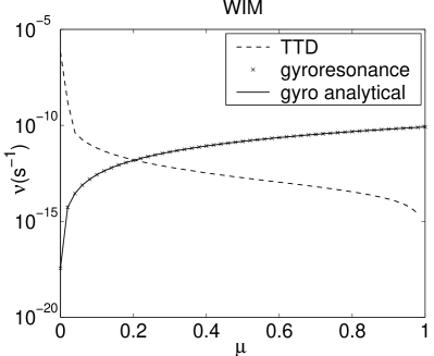
Figure 3: The scattering frequency $\nu$ vs. cosine of pitch angle $\mu$ of 1GeV CR (a) in halo, (b) in WIM. The ’x’ lines refer to scattering by gyroresonance and solid lines are the corresponding analytical results given by Eq.(32). The dashed lines are the results from Eq.(B49) for TTD. In (a), $\delta$ function and Breit-Weigner function match well except for the part marked by diamond symbols showing that $\delta$ function underestimate the contribution (see text).

It should be pointed out that all the results above are very much dependent on the plasma $\beta$, which is somewhat uncertain. But the basic conclusion is definite: fast modes dominate cosmic ray scattering except in very high $\beta$ medium where fast modes are severely damped. This demands a substantial revision of cosmic ray acceleration/propagation theories, and many related problems should be revisited.

5 Cosmic ray self confinement by streaming instability

When cosmic rays stream at a velocity much larger than Alfvén velocity, they can excite by gyroresonance MHD modes which in turn scatter cosmic rays back, thus increasing the amplitude of the resonant mode. This runaway process is known as streaming instability. It was claimed that the instability could provide confinement for cosmic rays with energy less than $\sim 10^{2}$GeV (Cesarsky 1980). However, this was calculated in an ideal regime, namely, there was no background MHD turbulence. In other words, it was thought that the self-excited modes would not be appreciably damped in fully ionized gas.

This is not true for turbulent medium, however. YL02 pointed out that the streaming instability is partially suppressed in the presence of background turbulence (see more in Lazarian, Cho & Yan 2003). More recently, detailed calculations of the streaming instability in the presence of background Alfvénic turbulence were presented in Farmer & Goldreich (2003), where the growth rate of the modes of wave number $k$ was assumed to be (Longair 1997)

$$\Gamma(k)=\Omega_{0}\frac{N(\geq E)}{n_{p}}(-1+\frac{v_{stream}}{V_{A}}),$$ (39a)

where $$N(\geq E) \geq E n_{p} N(\geq E)\simeq 2\times 10^{-10}(E/ )^{-1.6}$$ is the number density of cosmic rays with energy which resonate with the wave, is the number density of charged particles in the medium. The number density of cosmic rays near the sun is GeVcm^-3sr^-1 (Wentzel 1974).

Consider interaction with fast modes, which were shown earlier to dominate scattering. Such an interaction happens at the rate $\tau_{k}\sim(k/L)^{-1/2}V_{ph}/V^{2}$ (see Eq.(3)). By equating the growth rate Eq.((39a)) and the damping rate Eq.(3), we can find that the streaming instability is only applicable for particles with energy less than

$$\gamma_{max}\simeq 1.5\times 10^{-9}[n_{p}^{-1}(V_{ph}/V)(Lv\Omega_{0}/V^{2})^{0.5}]^{1/1.1},$$ (39b)

which for HIM, provides $\sim 20$GeV if taking the injection speed to be $V\simeq 25$km/s.

One of the most vital cases for streaming instability is that of cosmic ray acceleration in strong MHD shocks. Such shocks produced by supernovae explosions scatter cosmic rays by the postshock turbulence and by preshock magnetic perturbations created by cosmic ray streaming. The perturbations of the magnetic field may be substantially larger than the regular magnetic field. In this situation a different expression for the growth rate is applicable (Ptuskin & Zirakashvili 2003):

$$\Gamma(k)\simeq\frac{ak\epsilon U^{3}}{cV_{A}(\gamma_{max}^{a}-(1+a)^{-1})(kr_{g0})^{a}(1+A_{tot}^{2})^{(1-a)/2}},$$ (39c)

where $\epsilon$ is the ratio of the pressure of CRs at the shock and the upstream momentum flux entering the shock front, $U$ is the shock front speed, $a-4$ is the spectrum index of CRs at the shock front, $r_{g0}=c/\Omega_{0}$, $A_{tot}$ is the dimensionless amplitude of the random field $A_{tot}^{2}=\delta B^{2}/B_{0}^{2}$.

Magnetic field itself is likely to be amplified through an inverse cascade of magnetic energy at which perturbations created at a particular $k$ diffuse in $k$ space to smaller $k$ thus inducing inverse cascade. As the result the magnetic perturbations at smaller $k$ get larger than the regular field. As the result, even if the instability is suppressed for the growth rate given by eq. (39a) it gets efficient due to the increase of perturbations of magnetic field stemming from the inverse cascade.

Whether or not the streaming instability is efficient in scattering accelerated cosmic rays back depends on whether the growth rate of the streaming instability is larger or smaller than the damping rate. The precise picture of the process depends on yet not completely clear details of the inverse cascade of magnetic field. If, however, we assume that the small scale driving provides at the scales of interest isotropic turbulence the nonlinear damping happens on the scale of one eddy turnover time. If assuming the shock front speed $U$ is low enough, then the advection of the turbulence by shock flow is negligible and the perturbation $A_{tot}\ll 1$. In this case, we can get the maximum energy of particles accelerated in the shock by equating the growth rate of the instability Eq.(39c) to the damping rate due to turbulence cascade Eq.(3):

$$\gamma_{max}\simeq(\frac{a\epsilon(LeB_{0})^{0.5}U^{3}}{m^{0.5}V^{2}c^{2}})^{1/(0.5+a)}.$$ (39d)

From this we can estimate $\gamma_{max}\simeq 2\times 10^{7}(t/kyr)^{-9/4}$ in HIM.

As shown in the Eq.(39a) and (39c), the growth rate depends on the CRs’ density. In those regions where high energy particles are produced, e.g., shock fronts in ISM, $\gamma$ ray burst, SN, the streaming instability is more important.

6 Discussion

6.1 Applicability of our results

We have attempted to apply a new scaling relations obtained for MHD turbulence to the problem of cosmic ray scattering taking into account the turbulence cutoff arising from both collisional and collisionless damping. We considered both gyroresonance and transit-time damping (TTD).

In earlier papers it was frequently assumed that Alfvénic turbulence follows Kolmogorov spectrum while the problem of CR scattering was considered. This is incorrect because MHD turbulence is different from hydrodynamic turbulence if magnetic field is dynamically important. We appeal to the earlier research (see review by Cho & Lazarian 2003a) which showed that MHD turbulence can be decomposed into Alfvén, slow and fast modes. They have different statistics (see CL02). The Alfvén and slow modes follow GS95 scalings and show scale-dependent anisotropy.

Fast modes, however, are promising as a means of scattering due to their isotropy. Even in spite of the damping fast modes dominate scattering if turbulent energy is injected at large scales. We provided calculations for various phases of ISM, including galactic halo, WIM, HIM and partially ionized media. As the fast modes are subjected to different damping processes, the CR scattering varies. In galactic halo, the fast modes are subjected to collisionless damping. In WIM and HIM ion viscosity dominates the damping. All these damping increase with $\theta$ and marginal for parallel modes. As the result, the fast modes at small scales become anisotropic with $k_{\parallel}\gg k_{\perp}$. In this sense, fast modes have slab geometry but with less energies. These modes can efficiently scatter CRs through gyroresonance. TTD is more important for large pitch angle scattering and for the regime where fast modes are severely damped. We find that use of $\delta$ function entails errors and resonance broadening ought to be taken into account. The formal resonance peak $\cos\theta=V_{ph}/v_{\parallel}$ is smeared out because perturbations along the mean field $\nabla_{\parallel}\mathbf{B}$ is small for the quasi-perpendicular modes. In all the cases, the scattering efficiency decreases with plasma $\beta$ because the damping increases with $\beta$.

As every other model, the model adopted has its own limitations. For instance, within our model we did not consider wavelike component (see Montgomery & Turner 1981, Kinney & McWilliams 1998). Such parallel propagating fluctuations are observed in the solar wind (Matthaeus et al. 1990) and included in some of the existing models of cosmic ray transport (see Bieber et al. 1994). One could argue that such fluctuations could potentially be described by the weak turbulence model (see Galtier et al. 2000) or the weak turbulence model with imbalance (see a special case in Lithwick & Goldreich 2003).

However, weak balanced turbulence is known to have a limited inertial range: turbulence get strong very soon (see discussions of this point in Cho, Lazarian & Vishniac 2003). A work by one of us also shows that the same is true for the weak imbalanced turbulence. Therefore, while such type of turbulence could indeed be important near the sources of turbulence, its implications over vast spaces of interstellar gas are limited.

The same is true about our model of energy injection. We assume that the turbulent energy is being injected at large scales. While observations of power spectra are consistent with such a picture, it is clear that some energy is being injected at small scales. If the intensity of fluctuations produced by this local injection is higher than those created by the global turbulent cascade, such regions can be important places for scattering of cosmic rays. If Alfvénic turbulence which provides rather weak scattering when injected from large scales (Chandran 2000, YL02) were the only mechanism for scattering of cosmic rays, such localized regions of weak turbulence or intensive local injection of turbulent energy would be the dominant places of scattering. As we identified fast modes as an efficient source of scattering, in the zeroth approximation in our treatment we disregarded those localized sources of scattering.

We disregarded shocks as sources of scattering. We believe that shocks are more important means of cosmic ray acceleration than scattering. To simplify our model further we also disregarded magnetic mirrors created by molecular clouds (Chandran 2001), which statistics is uncertain and seem to be important most if other scattering means fail.

There are other simplifications that were adopted in the paper. For instance, our model disregarded complications associated with the large scale Alfvén perturbations. For the range of cosmic rays that we are dealing the Alfvén fluctuations are well within the inertial range and therefore various non-linearities are not important. Due to the same reasoning, we do not deal with the effects of ”bendover” associated with the energy injection scale (see Zank et al 1998).

Similarly, we do not deal with the gyroresonance scattering of the particles moving to magnetic field at angles close to 90 degrees. This allows us not to consider complex kinetic effects that are important for the small scale turbulence (compare Leamon et al. 1999). In addition, we did not consider effects of turbulence in partially ionized gas below the scale at which kinetic energy fluctuations are damped by the viscosity. This new regime of MHD turbulence arises in the partially ionized gas (Cho, Lazarian & Vishniac 2002) and is characterized by the high degree of magnetic field intermittency. While our simple estimates do not show that this regime is important for cosmic ray scattering, effects of magnetic intermittency on cosmic ray transport do require more work.

How good is the decomposition when the mean magnetic field is not strong is the issue that must still be tested. The decomposition procedure used in CL02 and CL03 requires existence of the mean magnetic field. However, one may argue (see CL03) that when mean magnetic field is weak, locally the nonzero magnetic field of larger eddies acts as the mean magnetic field for the smaller ones. Therefore physically the results obtained for the particular model could be argued to be valid even in the absence of the mean magnetic field. Testing this numerically is possible by taking volumes in the real space, defining there the local direction of the local mean field that changes from one volume to another (see Cho, Lazarian & Vishniac 2003 for a detailed discussion) and then using a decomposition in the Fourier space as this is done in CL02. For a present numerical studies this is extremely challenging, however. Nevertheless, the correspondence of properties of MHD turbulence with and without mean magnetic field reported in Cho & Lazarian (2003b) supports the theoretical expectations about the modes. One way or another, there are theoretical expectations that have been tested for the case most important for scattering of Galactic cosmic rays. These were being used for the present study.

Although scattering via fast modes is isotropic at large scales and becomes slab-type at small scales at which damping gets important, our model is radically different from earlier discussed 2D+slab and 3D+slab models (Bieber et al. 1994, Schlickeiser & Miller 1998).We used theoretically motivated models of turbulence that have been tested numerically. Therefore the transitions from one regime to another as well as the values of the intensity of perturbations have good justification within our approach.

We adopted a particular set of parameters of ISM while doing the calculation. The basic conclusion, namely, fast modes dominate the cosmic ray scattering, will remain the same even if the parameters are altered. However, since the $\beta$ value in ISM remains uncertain from observation, the damping scale $k_{c}$ is somewhat uncertain. And this determines the energy limit down to which gyroresonance is applicable.

6.2 Comparison with recent attempts in the same direction

An earlier attempt to study the effects of the GS95 scaling on the propagation of cosmic rays is made in Chandran (2000) and YL02 . These studies showed that Alfvén modes are not be efficient for cosmic ray scattering. Moreover, YL02 identified fast modes as the driver for cosmic ray scattering. As fast modes are subjected to damping it was not clear whether fast mode induced scattering is always efficient. This problem was dealt with in the present paper, which provides detailed calculations of the expected scattering rate by fast modes for various phases of the ISM and takes into account both gyroresonance and TTD scattering.

Another issue that this paper deals with is the suppression of the cosmic ray streaming instability by turbulence. This effect was first noticed in YL02 (see Lazarian, Cho & Yan (2003), Yan & Lazarian (2003) for more detail). The calculations of the effect were presented by Farmer & Goldreich (2004) for the weakly perturbed magnetic field. As the magnetic field may get strongly perturbed due to the inverse cascade of energy as the streaming instability develops first at smaller scales, in this paper we provide calculations of the suppression of the streaming instability for the strongly perturbed magnetic field.

7 Summary

In the paper above we characterized interaction of cosmic rays with balanced interstellar turbulence driven at a large scale. Our results can be summarized as follows:

1. Our calculations show that fast modes provide the dominant contribution to scattering of cosmic rays in different phases of interstellar medium provided that the turbulent energy is injected at large scales. This happens in spite of the fact that the fast modes are more subjected to damping compared to Alfvén modes.

2. As damping of fast modes depends on the angle between the magnetic field and the wave direction of propagation, we find that field wondering determined by Alfvén modes affects the damping of fast modes. At small scales the anisotropy of fast mode damping makes gyroresonant scattering within slab approximation applicable. At larger scales where damping is negligible the isotropic gyroresonant scattering approximation is applicable.

3. Transient time damping (TTD) provides an important means of how cosmic rays can be accelerated by fast modes. Use of $\delta$ function resonance entails errors, and therefore, resonance broadening is essential for TTD. Our study shows that it is vital for low energy and large pitch angle scattering. And it dominates scattering of cosmic rays in HIM and the partially ionized interstellar gas where fast modes are severely damped.

4. Streaming instability is subjected to non-linear damping due to the interaction of the emerging magnetic perturbations with the surrounding turbulence. The energy at which the streaming instability is suppressed depends on whether on the inverse cascade of magnetic energy as the instability gets more easily excited for low energy particles.

Appendix A A. Damping of MHD turbulence

Below we summarize the damping processes that we consider in the paper.

Ion-neutral damping

In partially ionized medium, viscosity of neutrals provides damping (see LY02). If the mean free path for a neutral atom, $l_{n}$, in a partially ionized gas with density $n_{tot}=n_{n}+n_{i}$ is much less than the size of the eddies under consideration, i.e. $l_{n}k\ll 1$, the damping time

$$\Gamma_{in}\sim\nu_{n}k^{2}\sim\left(\frac{n_{tot}}{n_{n}}\right)(l_{n}c_{n})k^{2},$$ (A1)

where $\nu_{n}$ is effective viscosity produced by neutrals. The mean free path of a neutral atom $l_{n}$ is influenced both by collisions with neutrals and with ions. The rate at which neutrals collide with ions is proportional to the density of ions, while the rate at which neutrals collide with other neutrals is proportional to the density of neutrals. The drag coefficient for neutral-neutral collisions is $\sim 1.7\times 10^{-10}T$(K)^0.3 cm³ s^-1 (Spitzer 1978), while for neutral-ion collisions it is $\sim{\langle v_{r}\sigma_{in}\rangle}\approx 1.9\times 10^{-9}$ cm³ s^-1 (Draine, Roberge & Dalgarno 1983). Thus collisions with other neutrals dominate for $n_{i}/n_{n}$ less than $\sim 0.09T^{0.3}$. Turbulent motions cascade down till the cascading time is of the order of $t_{damp}$. The maximal damping corresponds to $k^{-1}\sim l_{n}$. If the neutrals constitute less than approximately $5\%$, the cascade goes below $l_{n}$ and is damped at smaller scale (see below).

Collisionless damping

The nature of collisionless damping is closely related to the radiation of charged particles in magnetic field. Since the charged particles can emit plasma modes through acceleration (cyclotron radiation) and Cherenkov effect, they also absorb the radiation under the same condition (Ginzburg 1961). The thermal particles can be accelerated either by the parallel electric field which can also be called Landau damping or the magnetic mirror (TTD) associated with the comoving modes (or under the Cherenkov condition $k_{\parallel}v_{\parallel}=\omega$). The gyroresonance with thermal ions also causes the damping of those modes with frequency close to the ion-cyclotron frequency (Leamon et al. 1998), though it is irrelevant to the low frequency modes since we deal with GeV CRs here. The collisionless damping depends on the plasma $\beta\equiv P_{gas}/P_{mag}$ and the propagation direction of the modes. In general, the damping increases with the plasma $\beta$. And the damping is much more severe for fast modes than for Alfvén modes. For instance, the Alfvén modes are weakly damped even in a high $\beta$ medium, where fast modes are strongly damped. The damping rate $\gamma_{d}=\tau_{d}^{-1}$ of the fast modes of frequency $\omega$ for $\beta\ll 1$ and $\theta\sim 1$ (Ginzburg 1961) is

$$\Gamma_{L} = \frac{\sqrt{\pi\beta}}{4}\omega\frac{\sin^{2}\theta}{\cos\theta}\times[\sqrt{\frac{m_{e}}{m_{H}}}\exp(-\frac{m_{e}}{m_{H}\beta\cos^{2}\theta})+5\exp(-\frac{1}{\beta\cos^{2}\theta})],$$ (A2)

where $m_{e}$ is the electron mass. The exact expression for the damping of fast modes at small $\theta$ was obtained in Stepanov (1958)

$$\Gamma_{L}=\frac{\sqrt{\pi\beta}}{4}\omega\theta^{2}\times\left(1+\frac{\theta^{2}}{\sqrt{\theta^{4}+4\Omega_{i}^{2}/\omega^{2}}}\right)\sqrt{\frac{m_{e}}{m_{H}}}\exp(-\frac{m_{e}}{m_{H}\beta\cos^{2}\theta}).$$

When $\beta\gg 1$, we obtain the damping rate as a function of $\theta$ from Foote & Kulsrud 1979,

$$\Gamma_{L}=\frac{\sin^{2}\theta}{\cos^{3}\theta}\times\cases{2\omega^{2}/\Omega_{i}&for $k<\Omega_{i}/\beta V_{A}$\cr 2\Omega_{i}/\beta&for $k>\Omega_{i}/\beta V_{A}$\cr}$$ (A3)

where $\Omega_{i}$ is the ion gyrofrequency.

Ion viscosity

In a strong magnetic field ($\Omega_{i}\tau_{i}\gg 1$) the transport of transverse momentum is prohibited by the magnetic field. Thus transverse viscosity $\eta_{\perp}$ is much smaller than longitudinal viscosity $\eta_{0}=0.96n(T/eV)\tau_{i}$, $\eta_{\perp}\sim\eta_{0}/(\Omega_{i}\tau_{i})^{2}$. The heat generated by this damping is $Q_{vis}=\eta_{0}(\partial v_{x}/\partial x+\partial v_{y}/\partial y-2\partial v_{z}/\partial z)^{2}/3$, where $v_{x}$, $v_{y}$, $v_{z}$ are the velocity components of the wave perturbation (Braginskii 1965). From the expression, we see that the viscous damping is not important unless there is compression. Therefore Alfvén modes is marginally affected by the ion viscosity.

While the damping due to compression along the magnetic fields can be easily understood, it is counterintuitive that the compression perpendicular to the magnetic also results in damping through longitudinal viscosity. Following Braginskii (1965), the damping of perpendicular motion may be illustrated in the following way. To understand the physics of such a damping, consider fast modes in low $\beta$ medium. In this case, the motions are primarily perpendicular to the magnetic field so that $\partial v_{x}/\partial x=\dot{n}/n\sim\dot{B}/B$. The transverse energy of the ions increases because of the conservation of adiabatic invariant $v_{\perp}^{2}/B$. If the rate of compression is faster than that of collisions, the ion distribution in the momentum space is bound to be distorted from the Maxwellian isotropic sphere to an oblate spheroid with the long axis perpendicular to the magnetic field. As a result, the transverse pressure gets greater than the longitudinal pressure by a factor $\tau_{i}\sim\dot{n}/n$, resulting in a stress $\sim p\tau_{i}\dot{n}/n\sim\eta_{0}\partial v_{x}/\partial x$. The restoration of the equilibrium increases the entropy and causes the dissipation of energy with a damping rate $\Gamma_{ion}=k_{\perp}^{2}\eta_{0}/6\rho_{i}$ (Braginskii 1965).

In high $\beta$ medium, the velocity perturbations are radial as pointed out in $\S 2$. Thus $Q_{vis}=\eta_{0}(k_{x}v_{x}+k_{y}v_{y}-2k_{z}v_{z})^{2}/3=\eta_{0}k^{2}v^{2}(\sin^{2}\theta-2\cos^{2}\theta)^{2}/3$. Dividing this by the total energy associated with the fast modes $E_{k}=\rho_{i}v^{2}$, we can obtain the damping rate $\Gamma_{ion}=k^{2}\eta_{0}(1-3\cos^{2}\theta)^{2}/6\rho_{i}$.

All in all,

$$\Gamma_{ion}=\cases{k_{\perp}^{2}\eta_{0}/6\rho_{i}&for $\beta\ll 1$\cr k^{2}\eta_{0}(1-3\cos^{2}\theta)^{2}/6\rho_{i}&for $\beta\gg 1$\cr}$$ (A4)

Resistive damping

In the paper we ignore the resistive damping because of the following reason. The resistivity is much smaller than the longitudinal ion viscosity for fast modes. For parallel propagating fast modes which are not subjected to the viscous damping from the longitudinal viscosity, the resistive damping scale can be obtained by equating the damping rate $c^{2}k^{2}/8\pi\sigma_{\perp}$ with the cascading rate of the fast modes, where $\sigma_{\perp}\simeq 10^{13}(T/eV)^{3/2}$ (see Kulsrud & Pearce 1969) is the conductivity perpendicular to the magnetic field: $k_{res}^{-1}=1.8\times 10^{7}(L/pc)^{1/3}(T/10^{4}K)^{-1}(V_{A}/kms^{-1})^{-2/3}$cm. This scale turns out to be much smaller than the mean free path, where collisionless damping takes over. For Alfvén modes, the resistive damping rate is $\Gamma_{res}=c^{2}k_{\perp}^{2}/8\pi\sigma_{\parallel}$ (the term associated with $k_{\parallel}$is negligible because of anisotropy), where $\sigma_{\parallel}=1.96\sigma_{\perp}$is the conductivity parallel to the magnetic field. By equating it with the cascading rate of Alfvén modes, we can get the resistive damping scale $k_{res}^{-1}\simeq L(c^{2}/8\pi\sigma_{\parallel}V_{A}L)^{3/4}$. Comparing with the proton Larmor radius, we find $k_{res}^{-1}/r_{L}=3.6\times 10^{-3}(L/pc)^{1/4}(T/10^{4}K)^{-3/2}n^{1/2}(V_{A}/C_{s})^{1/4}$. It’s clear that in many astrophysical plasmas the resistive scale is less than proton Larmor radius. At this scale the energy can be transfered either to protons or to electron whistler modes. According to Cho & Lazarian (2004) whistler modes are even more anisotropic that the Alfvén ones. Therefore their heating of protons is unlikely. In terms of cosmic ray scattering they are of marginal importance.

Appendix B B. Fokker-Planck coefficients

In quasi-linear theory (QLT), the effect of MHD modes is studied by calculating the first order corrections to the particle orbit in the uniform magnetic field, and the ensemble-averaging over the statistical properties of the MHD modes (Jokipii 1966, Schlickeiser & Miller 1998). Obtained by applying the QLT to the collisionless Boltzmann-Vlasov equation, the Fokker-Planck equation is generally used to describe the evolvement of the gyrophase-averaged particle distribution. The Fokker-Planck coefficients $D_{\mu\mu},D_{\mu p},D_{pp}$ are the fundamental physical parameter for measuring the stochastic interactions, which are determined by the electromagnetic fluctuations:

$\begin{array}[]{cc}<B_{\alpha}(\mathbf{k})B_{\beta}^{*}(\mathbf{k^{\prime}})>=\delta(\mathbf{k}-\mathbf{k^{\prime}})P_{\alpha\beta}(\mathbf{k})&<B_{\alpha}(\mathbf{k})E_{\beta}^{*}(\mathbf{k^{\prime}})>=\delta(\mathbf{k}-\mathbf{k^{\prime}})T_{\alpha\beta}(\mathbf{k})\\ <E_{\alpha}(\mathbf{k})B_{\beta}^{*}(\mathbf{k^{\prime}})>=\delta(\mathbf{k}-\mathbf{k^{\prime}})Q_{\alpha\beta}(\mathbf{k})&<E_{\alpha}(\mathbf{k})E_{\beta}^{*}(\mathbf{k^{\prime}})>=\delta(\mathbf{k}-\mathbf{k^{\prime}})R_{\alpha\beta}(\mathbf{k}),\end{array}$

Adopting the approach in Schlickeiser & Achatz (1993), we can get the Fokker-Planck coefficients,

$$\left[\begin{array}[]{c}D_{\mu\mu}\\ D_{\mu p}\\ D_{pp}\end{array}\right] = {\frac{\Omega^{2}(1-\mu^{2})}{2B_{0}^{2}}}{\mathcal{R}}e\sum_{n=-\infty}^{n=\infty}\int_{\bf k_{min}}^{\bf k_{max}}dk^{3}\left[i\begin{array}[]{c}\left(1+\frac{\mu V_{A}}{v\zeta}\right)^{2}\\ \left(1+\frac{\mu V_{A}}{v\zeta}\right)mc\\ m^{2}c^{2}\end{array}\right]\int_{0}^{\infty}dte^{-i(k_{\parallel}v_{\parallel}-\omega+n\Omega)t}\left\{J_{n+1}^{2}({\frac{k_{\perp}v_{\perp}}{\Omega}})\left[\begin{array}[]{c}P_{{\mathcal{RR}}}({\mathbf{k}})\\ T_{{\mathcal{RR}}}({\mathbf{k}})\\ R_{{\mathcal{RR}}}({\mathbf{k}})\end{array}\right]\right.$$ (B10)

$$+ J_{n-1}^{2}({\frac{k_{\perp}v_{\perp}}{\Omega}})\left[\begin{array}[]{c}P_{{\mathcal{LL}}}({\mathbf{k}})\\ -T_{{\mathcal{LL}}}({\mathbf{k}})\\ R_{{\mathcal{LL}}}({\mathbf{k}})\end{array}\right]+J_{n+1}({\frac{k_{\perp}v_{\perp}}{\Omega}})J_{n-1}({\frac{k_{\perp}v_{\perp}}{\Omega}})\left.\left[e^{i2\phi}\left[\begin{array}[]{c}-P_{{\mathcal{RL}}}({\mathbf{k}})\\ T_{{\mathcal{RL}}}({\mathbf{k}})\\ R_{{\mathcal{RL}}}({\mathbf{k}})\end{array}\right]+e^{-i2\phi}\left[\begin{array}[]{c}-P_{{\mathcal{LR}}}({\mathbf{k}})\\ -T_{{\mathcal{LR}}}({\mathbf{k}})\\ R_{{\mathcal{LR}}}({\mathbf{k}})\end{array}\right]\right]\right\}$$ (B20)

where $|{\bf k_{min}}|=k_{min}=L^{-1}$, $|{\bf k_{max}}|=k_{max}$ corresponds to the dissipation scale, where $\zeta=1$ for Alfvén modes and $\zeta=k_{\parallel}/k$ for fast modes, $dk^{3}=2\pi k_{\perp}dk_{\perp}dk_{\parallel}$, $m=\gamma m_{H}$ is the relativistic mass of the proton, $v_{\perp}$ is the particle’s velocity component perpendicular to $\mathbf{B}_{0}$, $\phi=\arctan(k_{y}/k_{x}),$ ${\mathcal{L}},{\mathcal{R}}=(x\pm iy)/\sqrt{2}$ represent left and right hand polarization. For low frequency MHD modes, we have from Ohm’s Law $\mathbf{E}(\mathbf{k})=-(1/c)\mathbf{v}(\mathbf{k})\times\mathbf{B}_{0}$. So we can express the electromagnetic fluctuations $T_{ij},R_{ij}$ in terms of correlation tensors $K_{ij}$. For $\omega$ we use dispersion relations $\omega=k_{\parallel}V_{A}$ for Alfvén modes and $\omega=kV_{ph}$ for fast modes. Those dispersion relations were used to decompose and study the evolutions of MHD modes in CL02.

For gyroresonance, the dominant interaction is the resonance at $n=\pm 1$. By integrating over $\tau$, we obtain

$$\left(\begin{array}[]{c}D_{\mu\mu}\\ D_{\mu p}\\ D_{pp}\end{array}\right) = {\frac{\pi\Omega^{2}(1-\mu^{2})}{2}}\int_{\bf k_{min}}^{\bf k_{max}}dk^{3}\delta(k_{\parallel}v_{\parallel}-\omega+\pm\Omega)\left(\begin{array}[]{c}\left(1+\frac{\mu V_{ph}}{v\zeta}\right)^{2}\\ \left(1+\frac{\mu V_{ph}}{v\zeta}\right)mV_{A}\\ \iota^{2}m^{2}V_{A}^{2}\end{array}\right)$$ (B31)

$$\left\{(J_{2}^{2}({\frac{k_{\perp}v_{\perp}}{\Omega}})+J_{0}^{2}({\frac{k_{\perp}v_{\perp}}{\Omega}}))\left[\begin{array}[]{c}M_{{\mathcal{RR}}}({\mathbf{k}})+M_{{\mathcal{LL}}}({\mathbf{k}})\\ -C_{{\mathcal{RR}}}({\mathbf{k}})-C_{{\mathcal{LL}}}({\mathbf{k}})\\ K_{{\mathcal{RR}}}({\mathbf{k}})+K_{{\mathcal{LL}}}({\mathbf{k}})\end{array}\right]\right.$$

$$- 2J_{2}({\frac{k_{\perp}v_{\perp}}{\Omega}})J_{0}({\frac{k_{\perp}v_{\perp}}{\Omega}})\left.\left[e^{i2\phi}\left[\begin{array}[]{c}M_{{\mathcal{RL}}}({\mathbf{k}})\\ -C_{{\mathcal{RL}}}({\mathbf{k}})\\ K_{{\mathcal{RL}}}({\mathbf{k}})\end{array}\right]+e^{-i2\phi}\left[\begin{array}[]{c}M_{{\mathcal{LR}}}({\mathbf{k}})\\ -C_{{\mathcal{LR}}}({\mathbf{k}})\\ K_{{\mathcal{LR}}}({\mathbf{k}})\end{array}\right]\right]\right\},$$ (B38)

where $\iota=1$ for low $\beta$ medium and $\iota=\sin^{2}\theta$ for high beta medium.

For TTD,

$$\left(\begin{array}[]{c}D_{\mu\mu}\\ D_{\mu p}\\ D_{pp}\end{array}\right) = {\frac{\pi\Omega^{2}(1-\mu^{2})}{2}}\int_{\bf k_{min}}^{\bf k_{max}}dk^{3}\frac{\tau_{k}}{\tau_{k}^{2}+(k_{\parallel}v_{\parallel}-\omega)^{2}}\left(\begin{array}[]{c}\left(1+\frac{\mu V_{ph}}{v\zeta}\right)^{2}\\ \left(1+\frac{\mu V_{ph}}{v\zeta}\right)mV_{A}\\ \iota^{2}m^{2}V_{A}^{2}\end{array}\right)$$ (B49)

$$2J_{1}^{2}({\frac{k_{\perp}v_{\perp}}{\Omega}})\left[\begin{array}[]{c}M_{{\mathcal{RR}}}({\mathbf{k}})+M_{{\mathcal{LL}}}({\mathbf{k}})+e^{i2\phi}M_{{\mathcal{RL}}}({\mathbf{k}})+e^{-i2\phi}M_{{\mathcal{LR}}}({\mathbf{k}})\\ -C_{{\mathcal{RR}}}({\mathbf{k}})-C_{{\mathcal{LL}}}({\mathbf{k}})-e^{i2\phi}C_{{\mathcal{RL}}}({\mathbf{k}})-e^{-i2\phi}C_{{\mathcal{LR}}}({\mathbf{k}})\\ K_{{\mathcal{RR}}}({\mathbf{k}})+K_{{\mathcal{LL}}}({\mathbf{k}})+e^{i2\phi}K_{{\mathcal{RL}}}({\mathbf{k}})+e^{-i2\phi}K_{{\mathcal{LR}}}({\mathbf{k}})\end{array}\right]$$

Define the integrand

$$G(\mathbf{k}) = (J_{2}^{2}({\frac{k_{\perp}v_{\perp}}{\Omega}})+J_{0}^{2}({\frac{k_{\perp}v_{\perp}}{\Omega}}))(K_{{\mathcal{RR}}}({\mathbf{k}})+K_{{\mathcal{LL}}}({\mathbf{k}}))-2J_{2}({\frac{k_{\perp}v_{\perp}}{\Omega}})J_{0}({\frac{k_{\perp}v_{\perp}}{\Omega}})(e^{i2\phi}K_{{\mathcal{RL}}}({\mathbf{k}})+e^{-i2\phi}K_{{\mathcal{LR}}}({\mathbf{k}}))$$

$$T(\mathbf{k}) = 2J_{1}^{2}({\frac{k_{\perp}v_{\perp}}{\Omega}})((K_{{\mathcal{RR}}}({\mathbf{k}})+K_{{\mathcal{LL}}}({\mathbf{k}})+(e^{i2\phi}K_{{\mathcal{RL}}}({\mathbf{k}})+e^{-i2\phi}K_{{\mathcal{LR}}}({\mathbf{k}}))$$ (B50)

. We shall show below how they can be simplified in various cases to enable an analytical evaluation of the integral. The spherical components of the correlation tensors are obtained in the following.

For Alfvén modes, their tensors are proportional to

$$I_{ij}=\left(\begin{array}[]{cc}\sin^{2}\phi&-\cos\phi\sin\phi\\ -\cos\phi\sin\phi&\cos^{2}\phi\end{array}\right).$$

For Alfvén modes, $k_{\perp}v_{\perp}/\Omega\gg 1$ because of the anisotropy. So we can use the asymptotics of the Bessel function $J_{n}(x)=\sqrt{2/\pi x}\cos(x-n\pi/2-\pi/4)$ when $x\rightarrow\infty$. Thus from Eq.(8), we simplify the integrand in Eq.(24), $G({\mathbf{k}})\propto k_{\perp}^{-10/3}\exp(-L^{1/3}|k_{\parallel}|/k_{\perp}^{2/3}),$ the integral of which will be $\propto(|k_{\parallel}|L^{1/3})^{-6.5}\Gamma[6.5,k_{max}^{-2/3}|k_{\parallel}|L^{1/3}]$. Then from Eq.(24) we can get the analytical result for the scattering by Alfvén modes as given in Eq.(25).

For fast modes, their magnetic correlations have such forms

$$M_{ij}\propto\left(\begin{array}[]{ccc}\cos^{2}\theta\cos^{2}\phi&\cos^{2}\theta\cos\phi\sin\phi&\cos\theta\sin\theta\cos\phi\\ \cos^{2}\theta\cos\phi\sin\phi&\cos^{2}\theta\sin^{2}\phi&\cos\theta\sin\theta\sin\phi\\ \cos\theta\sin\theta\cos\phi&\cos\theta\sin\theta\sin\phi&\sin^{2}\theta\end{array}\right).$$

Their velocity correlations are

$$K_{ij}\propto\left(\begin{array}[]{ccc}\cos^{2}\phi&\cos\phi\sin\phi&0\\ \cos\phi\sin\phi&\sin^{2}\phi&0\\ 0&0&0\end{array}\right).$$ (B54)

for $\beta\ll 1$ and $K_{ij}\propto k_{i}k_{j}/k^{2}$ for $\beta\gg 1$.

In general, it’s more difficult to solve the integral in Eq.(B20) for the fast modes because they are isotropic. However, if taking into account damping, Bessel function can be evaluated using the zeroth order approximation. Thus from Eq.(24,B,B54), we see for gyroresonance the integrand can be simplified as $G(\mathbf{k})\propto(J_{2}-J_{0})^{2}k^{-7/2}\propto k^{-7/2}$. For TTD, $T(\mathbf{k})\propto J_{1}^{2}(k_{\perp}v_{\perp}/\Omega)k^{-7/2}\propto k^{-3/2}v_{\perp}^{2}\sin^{2}\theta\propto k^{-3/2}v_{\perp}^{2}(1-V_{ph}^{2}/v_{\parallel}^{2})$. Then we can solve the integral in Eq.(B49) analytically and get the scattering rate for fast modes.

References

- (1) Alfvén, H. & F’́althammar, C.G. 1963, Cosmical Electrodynamics, Oxford, Clarendon Press
- (2) Armstrong, J. W., Rickett, B. J., & Spangler, S. R. 1995, 443, 209
- (3) Beck, R., Space Sci. Rev., 99, 243 (2001)
- (4) Berezinskii, V., Bulanov, S., Dogiel, S., Ginzburg, V. & Ptuskin, V., Astrophysics of Cosmic Rays (North-Holland, New York, 1990)
- (5) Bieber, J. W., Smith, C. W., & Matthaeus, W. H. 1988, ApJ, 334, 470
- (6) Bieber, J.W., Matthaeus, W. H., & Smith, C. W. 1994, ApJ, 420, 294
- (7) Braginskii, S.I. 1965, Rev. Plasma Phys. 1, 205
- (8) Cesarsky, C. 1980, Annu. Rev. Astr. Ap., 18, 289
- (9) Chandran, B. 2000, Phys. Rev. Lett., 85(22), 4656
- (10) Cho, J., Lazarian, A. & Vishniac, E.T. 2002, ApJ, 564, 291 (CLV02)
- (11) Cho, J., Lazarian, A. & Vishniac, E.T. 2003, in Simulations of magnetohydrodynamic turbulence in astrophysics, eds. T. Passot & E. Falgarone (Springer LNP, 614, 56)
- (12) Cho, J., Lazarian, A. & Yan, H. 2002, Seeing Through the Dust: The Detection of HI and the Exploration of the ISM in Galaxies, ASP Conference Proceedings, Vol. 276. Edited by A. R. Taylor, T. L. Landecker, and A. G. Willis, p.170
- (13) Cho, J. & Lazarian, A. 2002, Phys. Rev. Lett., 88, 245001 (CL02)
- (14) Cho, J. & Lazarian, A. 2003a, astro-ph/0301462
- (15) Cho, J. & Lazarian, A. 2003b, MNRAS, 345, 325 (CL03)
- (16) Cho, J. & Lazarian, A. 2004, submitted to Phys. Rev. Lett.
- (17) Cho, J. & Vishniac, E. T. 2000, ApJ, 539, 273
- (18) Farmer, A. & Goldreich, P. 2003, astro-ph/0311400
- (19) Fisk, L. A., Goldstein, M. L., & Sandri, G. 1974, ApJ, 190, 417
- (20) Foote, E.A. & Kulsrud, R.M. 1979, ApJ, 233, 302
- (21) Garcia Munoz, M. Simpson, J.A., Guzik, T.G., Wefel, J.F. & Margollis, S.H. 1987, ApJs, 64, 269
- (22) Ginzburg, V. L. 1961, Propagation of Electromagnetic Waves in Plasma (New York: Gordon & Breach)
- (23) Goldreich, P. & Sridhar, H. 1995, ApJ, 438, 763
- (24) Goldstein, M. L. 1976, ApJ, 204, 900
- (25) Jokipii, J. R. 1966, ApJ, 146, 480
- (26) Higdon, J. C. 1984, ApJ, 285, 109
- (27) Kinney, R. M. & McWilliams, J. G. 1998, Phys. Rev. E, 57, 7111
- (28) Kulsrud, R. & Pearce, W.P. 1969, ApJ, 156, 445
- (29) Lazarian, A. & Cho, J. 2003, in Magnetic fields and Star Formation, Spain, ApSS, astro-ph/0311372
- (30) Lazarian, A., Petrosian, V., Yan, H. & Cho, J. 2002, Review at the NBSI workshop ‘Beaming and Jets in Gamma Ray Bursts‘, ed. R. Ouyed, astro-ph/0301181
- (31) Lazarian, A. & Pogosyan, D. 2000, ApJ, 537, 720
- (32) Lazarian, A. & Vishniac, E. 1999, ApJ, 517, 700L
- (33) Leamon, R,J., Matthaeus, W.H., & Smith, C.W. 1998, ApJ, 507, 181L
- (34) Lerche, I. & Schlickeiser, R. 2001, A&A, 378, 279
- (35) Lithwick, Y. and Goldreich, P. 2001, ApJ, 562, 279
- (36) Lithwick, Y. and Goldreich, P. 2003, ApJ, 582, 1220L
- (37) Longair, M.S. 1997, High Energy Astrophysics ( Cambridge University Press, 1997)
- (38) Mac Low, M.-M. 2002, Ap&SS, 390, 307
- (39) Matthaeus, W. H., Goldstein, M. L., & Roberts, D. A. 1990, J. Geophys. REs., 95, 20,673
- (40) Maron, J. & Goldreich, P. 2001, 554, 1175
- (41) Miller, J A. 1997, ApJ 491, 939 (2001)
- (42) Montgomery, D.; Turner, L. 1981, Phys. Fluids, 24, 825
- (43) Montgomery, D., Brown, M. R., & Matthaeus, W. H. 1987, J. Geophys. Res. 92, 282
- (44) Owens, A. J. 1974, ApJ, 191, 235
- (45) Pryadko, J.M. & Petrosian, V. 1999, ApJ, 515, 873
- (46) Ptuskin, V. S. & Zirakashvili, V. N. 2003, A& A, 403, 1
- (47) Schlickeiser, R. & Achatz, U. 1993, J. Plasma Phy. 49, 63
- (48) Schlickeiser, R. & Miller, J.A. 1998, ApJ, 492, 352
- (49) Schlickeiser, R. 2002, Cosmic Ray Astrophysics (Spinger-Verlag: Berlin Heidelberg)
- (50) Seo, E.S. & Ptuskin, V.S. 1994, ApJ, 431, 705
- (51) Shebalin, J. V., Matthaeus, W. H., & Montgomery, D. 1983, 29, 525
- (52) Shebalin, J. V., & Montgomery, D. 1988, J. Plasma Phys. 39, 339
- (53) Wentzel, D. G. 1974, ARA&A, 12, 71
- (54) Stanimirovic, S. & Lazarian, A. 2001, ApJ, 551, L53
- (55) Webber, W.R. 1993, ApJ, 402, 188
- (56) Yan, H. & Lazarian, A. 2002, Phys. Rev. Lett., 89, 281102 (YL02)
- (57) Yan, H. & Lazarian, A. 2003, astro-ph/0311369
- (58) Zank, G.P. & Matthaeus, W. H. 1992, J. Plasma Phys. 48,85
- (59) Zank, G.P., Matthaeus, W. H., Bieber, J. W., & Moraal, H. 1998, J. Geophys. Res. 103, 2085