A Determination of the Chemical Composition of $\alpha$ Centauri A from Strong Lines

Nimish Pradumna Hathi

Department of Physics

The University of Queensland

Brisbane, Australia.

Supervisor: Dr. B. J. O’Mara
Submitted: April 1997

Accepted: August 1997

A thesis submitted to the University of Queensland in
fulfilment of the requirements for the degree of Master of Science

Abstract

The abundance of iron, magnesium, calcium and sodium in $\alpha$ Centauri A ($\alpha$ Cen A) is determined from strong lines of these elements using the theory of collisional line broadening of alkali and other spectral lines by neutral hydrogen developed by Anstee & O’Mara [1] and the spectrum synthesis program of John Ross [2]. The derived abundance is independent of non–thermal motions in the photosphere and is in good agreement with the results obtained by Chmielewski et al. [3] and Furenlid & Meylan [4] within the uncertainties involved.

As the abundances are derived from the wings of strong lines they are independent of non–thermal motions in the photosphere of $\alpha$ Cen A. The microturbulence is then determined using medium–strong lines of iron by fixing the abundance of iron to the value determined from the strong lines of iron, and adjusting the microturbulence to match the observed equivalent width of each line. The microturbulence is the average of the values obtained for all lines. This microturbulence can then be used in determination of the abundance of other elements for which there are no strong lines in the spectrum.

The abundances of iron, magnesium, calcium and sodium in $\alpha$ Cen A are approximately 0.2 dex higher than in the Sun. Also the microturbulence in the atmosphere of $\alpha$ Cen A which is (with the aid of the improved theory of line broadening) determined independently of the abundances is 1.34 km/s i.e., 0.20 km/s greater than on the Sun.

Chapter 1 Introduction

A sound procedure for the determination of chemical composition of the Sun and stars is important if we are to understand how elements are synthesised by thermonuclear burning in stellar interiors, and how, in turn, this relates to the chemical evolution of galaxies. The Sun and stars with similar surface temperatures are important as lines of neutral and singly ionised metals are prevalent in these stars allowing abundances to be determined for a wide selection of elements. The chemical composition of the Sun is particularly important as it is used as a standard to which all other stars are referenced. The lines best suited to abundance determinations are strong lines as their wings are not affected by uncertainties in the line of sight motions (microturbulence) of the absorbing atoms and their intrinsic strengths (f–values) can be accurately determined in the laboratory.

In the past, a major impediment to the use of such lines has been the lack of an adequate theory for the broadening of these lines by collisions with neutral hydrogen atoms. Recently Anstee & O’Mara (1991) [1] developed a theory which they tested by applying it to the sodium D–lines in the solar spectrum. Anstee & O’Mara (1995) [5] used the theory to construct tables of line broadening cross–sections for s–p, p–s transitions covering a range of effective principal quantum numbers for the upper and lower levels of the transition. Anstee, O’Mara & Ross (1997) [9] used these data in the determination of the solar abundance of iron from the strong lines of Fe I. The derived abundance was in excellent agreement with the meteoritic value ending a long standing controversy about possible deviations of the solar abundance from the meteoritic value. As a result of this work abundances can now be derived with some confidence from strong lines with the resulting abundance being independent of non–thermal motions in the photosphere.

In the past medium–strong lines have often been used whose equivalent widths are sensitive to non–thermal motions in the stellar photosphere, and consequently it has been difficult to determine whether the chemical composition of a star like $\alpha$ Cen A differs from that of the Sun. For example, Bessell (1981) [10] obtained a solar composition for this star assuming a microturbulence of 1.7 km/s while more recently Furenlid & Meylan (1990) [4] and Chmielewski et al. (1992) [3] in an analysis of $\alpha$ Cen A & B using a microturbulence of 1.0 km/s find that the abundance of iron is systematically greater than in the Sun by 0.12 and 0.22 dex respectively. On the other hand, if strong lines are used an abundance of iron can be derived which is independent of any assumed microturbulence. Moreover, once the abundance of iron has been determined in this manner, the microturbulence can be uniquely determined by requiring the abundance derived from medium–strong lines match that derived from the strong lines. In this way the derived abundance and the microturbulence can be decoupled leading to independent values for both. The derived microturbulence can then be used in the determination of the abundance of elements for which there are no strong lines in the star. It is the purpose of this thesis to test this new method of analysis by application to the chemical composition of $\alpha$ Cen A.

A brief review of the thesis contents:

In Chapter 2, the literature review of work on $\alpha$ Cen is presented which includes its physical properties and results obtained for its chemical composition.

In Chapter 3, the theory of the broadening of spectral lines by collisions with atomic hydrogen is reviewed, with emphasis on the more recent work of Anstee & O’Mara (1991) [1] and Anstee & O’Mara (1995) [5].

In Chapter 4, the spectrum synthesis software used in the thesis is applied to selected medium–strong lines of Fe I in the solar spectrum to deduce the microturbulence required to bring the abundance derived from strong and medium–strong lines in the solar spectrum into agreement; a preview of the analysis to be carried out on $\alpha$ Cen A.

In Chapter 5, the $\alpha$ Cen system is described and the spectra obtained for $\alpha$ Cen A & B are described along with the process of reducing these data for analysis by the spectrum synthesis program and identification of the lines.

In Chapter 6, abundances are derived from the strong and medium–strong lines in $\alpha$ Cen A and a microturbulence is derived.

In Chapter 7, conclusions of the analysis carried out in this thesis are summarized and suggestions are made for future work.

Chapter 2 Literature Review

The nearest star to our solar system, $\alpha$ Cen, is in fact a system of three stars viz $\alpha$ Cen A, $\alpha$ Cen B and Proxima Cen. The star system $\alpha$ Cen, one of the pointers to the Southern Cross, comprises of a –0.3 magnitude visual binary consisting of $\alpha$ Cen A, a G2V star (very similar to the Sun) and $\alpha$ Cen B a K0V star. The orbital period is 80.089 years, the semi–major axis is 23.5 AU, the distance 1.33 pc, the masses are 1.11 and 0.92 ($\pm$ 0.03)$M_{\odot}$. The third star Proxima Cen is closer to the Sun than any other star. They are all about 4 light years away. They lie in the constellation Centaurus, in the Milky Way and are visible from the Southern Hemisphere.

No less than 229 bibliographic references are given for $\alpha$ Cen A in the SIMBAD (Set of Identification, Measurements and Bibliography for Astronomical Data 1991 edition) and 140 references for $\alpha$ Cen B [3]. According to SIMBAD the first detailed analyses of $\alpha$ Cen A and $\alpha$ Cen B were done only in 1970 by French and Powell [11].

Recent detailed investigations of composition, temperature and ages of $\alpha$ Cen A and B have been in agreement in their conclusion that $\alpha$ Cen A has temperature a little higher or nearly equal to the Sun, is more metal–rich and is of the same age as or older than the Sun (note that older stars usually have a lower metallicity than the Sun). Exceptions are Bessell [10], whose analysis gives $\alpha$ Cen A and B having the same abundance as the Sun and Furenlid & Meylan [4] concluded that the effective temperature of $\alpha$ Cen A is 5710 K, which is 70 K less than that of the Sun (here adopted solar effective temperature is 5780 K).

Here is a brief summary of what some investigators have to say about $\alpha$ Cen A.

Blackwell & Shallis [12] describe the infrared flux method of determining stellar angular diameters. The accuracy of the method is tested on Arcturus and twenty seven other stars including $\alpha$ Cen A. Given the angular diameter, $\theta$, the effective temperature, $T_{e}$, is derived from the integrated flux from the star at the earth, $F_{E}$ , through the defining relation

$$\sigma T^{4}_{e}=4*F_{E}/\theta^{2},$$ (2.1)

or alternatively given $F_{E}$ and the flux ($T_{e}$) from a suitable model atmosphere, $\theta$ can be obtained. Their result for $\alpha$ Cen A, using the adopted effective temperature of 5800 K, gives an angular diameter of $(86.2\pm 2.3)*10^{-4}$ arcsec. The advantage of this method is that it is applicable to cool stars, if a reasonably good model atmosphere is available.

Bessell [10], using a grid of unpublished line blanketed models of Gustafsson, Bell, Nordlund, Eriksson (1979) analysed Fe and Ti lines to obtain the abundance of these elements in $\alpha$ Cen A (and B). In his analysis Bessell [10] obtained abundance of Fe and Ti in $\alpha$ Cen A equal to the solar values. Two important parameters in this analysis were found to have higher values. One was the adopted effective temperature of 5820 K which is 40 K higher than the effective temperature of the Sun and the other was a higher microturbulence of 1.7 km/s, which Bessell [10] concluded must have contributed to above solar equivalent widths of lines in $\alpha$ Cen A. Other investigators do not agree with Bessell [10] regarding this higher microturbulence.

Soderblom and Dravins [13] measured the lithium abundance in $\alpha$ Cen A. On a scale where log N(H) = 12.00, they found a lithium abundance of log N(Li) = 1.28, which is nearly twice that of the Sun. As it is difficult to estimate the age of a star from the lithium abundance alone, they assume that the age of $\alpha$ Cen A, depending on the composition, could be as low as 4 Gyr, or as great as 8 Gyr. In this analysis Soderblom and Dravins [13] support an effective temperature of $\alpha$ Cen A which is same as the Sun. Their conclusion that $\alpha$ Cen A has twice the lithium abundance compared to the Sun is consistent with its greater mass (1.1$M_{\odot}$), despite their prediction of probable evolutionary age of $\alpha$ Cen A to be 6 Gyr.

Soderblom [14], later in 1986, concluded that there is a good agreement between the (wings of) H$\alpha$ profiles of $\alpha$ Cen A and the Sun which suggests they have the same effective temperature. Using this temperature and adopted luminosities he calculated the radius of $\alpha$ Cen A as 1.23$R_{\odot}$.

A differential abundance analysis between $\alpha$ Cen A and the Sun has been carried out by Furenlid & Meylan [4]. They have measured around 500 lines of 26 elements in very high $S/N$ ratio (500–10,000) spectra for both objects. They find that the absorption lines in $\alpha$ Cen A are on average around 10 mÅ stronger than the Sun. In their analysis Furenlid & Meylan [4] found that there is an average metal overabundance in $\alpha$ Cen A of around 0.12 dex ($\pm$ 0.02 to $\pm$ 0.04 dex) on scale of log N(H) = 12.0. The average abundance of Fe, Mg and Si relative to the Sun was found to be 0.20 dex, using an effective temperature of 5800 K, log g = 4.0 and microturbulence $\xi$ = 1.0 km/s. The effective temperature is reduced to 5710 K and the overabundance of Fe reduces from 0.20 to 0.11 dex, when effects of the abundance on continuous absorption are taken into account. It is unusual to find so low an effective temperature as no other investigator has come up with this conclusion. Furenlid & Meylan [4] determined age of $\alpha$ Cen A to be 4.2 $\pm$ 0.4 billion years which is nearly same as that of the Sun.

A detailed abundance study for $\alpha$ Cen A and $\alpha$ Cen B was carried out by Chmielewski et al. [3]. Using high quality spectra with high $S/N$ ratio and high resolution, they have estimated the effective temperature, iron abundance and lithium abundance. The values they obtained are as follows : $T_{eff}$ = 5800 K, [Fe/H] = +0.22 $\pm$ 0.02 and log N(Li) = 1.4 $\pm$ 0.3. Their observations of the Ca II infrared triplet indicate a low level of chromospheric activity for $\alpha$ Cen A and B compared to the Sun. From the abundance analysis they are able to confirm that $\alpha$ Cen A is a Metal–Rich (MR) star.

Chmielewski et al. [3] have summarised recent studies on $\alpha$ Cen A. Table 2.1 summarises important analysis results for $\alpha$ Cen A (here results of Chmielewski et al. [3] are also included).

Table 2.1: Results from Recent Analysis for $\alpha$ Cen A.

Analysis	Teff K	log g	$\xi$ km/s	[Fe/H] dex
$[11]$	5770 $\pm$ 70	–	–	+0.22 $\pm$ 0.05
$[10]$	5820	4.25	1.7	–0.01
$[13]$	5770 $\pm$ 20	–	–	–
$[4]$	5710 $\pm$ 25	4.0 $\pm$ 0.2	1.0	+0.12 $\pm$ 0.02
$[3]$	5800 $\pm$ 20	4.31 $\pm$ 0.02	1.0	+0.22 $\pm$ 0.02

The metallicity of $\alpha$ Cen A has been discussed by Noels et al. [15], Neuforge [16] and Fernandes & Neuforge [17]. All three papers have used different calibration techniques and predicted that the metallicity is high in $\alpha$ Cen A compared to the Sun by a factor of 2 (0.3 dex). Noels et al. [15] using a generalisation of the solar calibration technique computed evolutionary sequences for 1.085$M_{\odot}$ with different values of Z, Y, and $\alpha$. They found that, the fraction by mass of elements more massive than He, Z = 0.04, the helium mass fraction, Y $\sim$ 0.32 and convection parameter $\alpha$ = 1.6, where $\alpha$ is the ratio of the mixing length to the pressure scale height i.e.$(l/H_{p})$. The helium abundance is higher than that of the Sun, which is nearly equal to 0.28. They adopted mean values of effective temperature as 5765 K and Luminosity log (L/$L_{\odot}$) = 0.1853.

Neuforge [16] used the same calibration technique as that of Noels et al. [15] but used different opacities and effective temperature. She computed her own set of low temperature atmospheric opacities for different values of Z ranging from 0.02 to 0.04. She adopted the effective temperature from Chmielewski et al. [3] which is 5800 K $\pm$ 20 K. Neuforge [16] found the values for metallicity Z = 0.038, helium Y = 0.321, age t = 4.84 Gyr and convection parameter $\alpha$ = 2.10. The value of the convection parameter $\alpha$ is different from Noels et al. [15] only because of different opacities.

Fernandes and Neuforge [17] discuss two calibration techniques for fixed Z and varied Z, using models calculated with mixing length convection theory (MLT) and explain their solution through the behaviour of the convection parameter $\alpha$ with chemical composition. They also predicted a higher Z for $\alpha$ Cen A compared to the Sun from their analysis.

Chapter 3 Theory of Spectral Line Broadening

3.1 Introduction to Line Broadening

Broadening of spectral lines in stellar atmospheres is mainly due to three mechanisms. They are:

• Natural broadening, due to the finite lifetimes of the upper and lower levels.

• Collisional broadening, caused by perturbations of atomic energy levels during collisions with other particles. There are two main sources of collisional broadening in solar–type stellar atmospheres viz :

  • Stark broadening, due to collisions with electrons and

  • so called van der Waals broadening, due to collisions with atoms, mainly neutral hydrogen.

• Doppler broadening, caused by random motions of the absorbing and emitting atoms along the line of sight. These random motions may be due to:

  • thermal motions of the atoms in the gas (thermal broadening) or

  • non–thermal random motions due to some form of small scale turbulence (microturbulence).

Natural broadening and Doppler broadening are always present and dominate the shapes near the line centre at low densities. However, natural broadening is important only in the cores of strong lines formed in the upper layers of the stellar atmospheres. The line shapes are strongly influenced by interactions of the radiating atoms or ions with surrounding particles. Then the Collisional broadening (Pressure broadening) comes into the picture. The most important interactions are those between radiating systems and electrons. Because electric fields are involved, this type of broadening is called Stark broadening. In the atmospheres of hot stars, electron collisions are the most important because electrons are the dominant particle species, they move rapidly and interact strongly with the absorbing atoms. On the other hand, the outer layers of the Sun and stars of similar effective temperature are sufficiently hot to dissociate molecular hydrogen into atomic hydrogen but are insufficiently hot to ionize hydrogen. The few electrons present result from thermal ionisation of metals such as iron and as a result of the low abundance of the metals, hydrogen atoms outnumber electrons by about 10,000:1. The collisional broadening of absorption lines in these stars is therefore dominated by collisions with atomic hydrogen.

In addition to the above classification of the various pressure broadening mechanisms, there is the division into impact (collision) and quasi–static (statistical) broadening. These are two extreme approximations in the general theory of broadening. The quasi–static description is valid when the perturbers move relatively slowly, so that the perturbation is practically constant over the time of interest, which is, at most, of the order of the inverse of the line width, the latter being measured in angular frequency units. In the impact approximation, on the same time scale, the duration of individual collisions is negligibly small which is always the case for broadening by collisions with electrons and hydrogen atoms.

As collisions with hydrogen atoms dominate the collisional broadening of lines in cool stars like the Sun, it is important to have a satisfactory theory for this line broadening process if strong lines are to be used in determination of the chemical composition of these stars.

3.2 Broadening by Collisions with Hydrogen Atoms

A theory for the broadening of spectral lines by collisions with atomic hydrogen developed by Anstee & O’Mara [1] is described in a paper presented by O’Mara [18] at an IAU Conference in Sydney in January 1997. An extract from that paper is quoted below.

“In cool stars neutral hydrogen atoms outnumber electrons by four orders of magnitude, consequently the broadening of most spectral lines is dominated by collisions with neutral hydrogen atoms. Conventional vander Waals’ theory for this broadening process is known to underestimate the broadening of spectral lines in the Sun by about a factor of two. Development of a satisfactory theory is important as it would allow strong lines with well determined f–values to be used to determine abundances in cool stars in a manner which is independent of photospheric motions. Also such lines could also be used to determine surface gravities in cool stars.

Collisions with neutral hydrogen atoms are sufficiently fast for the impact approximation of spectral line broadening theory to be valid. In this approximation the line has a Lorentz profile with a half half–width which is given by:

$$w=N\int_{0}^{\infty}vf(v)\sigma(v)dv,$$ (3.1)

where $N$ is the hydrogen atom number density, v is the relative collision speed, f(v) is the speed distribution and the line broadening cross–section

$$\sigma(v)=2\pi\int_{0}^{\infty}<\Pi(b,v)>_{av}bdb,$$ (3.2)

where the integrand contains the product of the geometrical cross–section 2$\pi bdb$ and a line broadening efficiency factor $<\Pi(b,v)>_{av}$ for collisions with impact parameter b and relative speed v.

$<...>_{av}$ indicates that the efficiency factor has to be averaged over all orientations of the perturbed atom. The efficiency factor can be expressed in terms of the S–matrix elements for the collision which are functionally dependent on the interaction energy between a hydrogen atom in the ground state and the perturbed atom in its upper and lower states. The only essential difference between various theoretical treatments is in the method employed to determine this interaction energy.

In the theory developed by Anstee & O’Mara [1] the interaction energy is calculated using Rayleigh–Schrödinger perturbation theory. If exchange effects are neglected, the shift in energy of the two–atom system as a result of the electrostatic interaction V between them is given by

$$\Delta E_{i}=<i|V|i>+\sum_{j\neq i}\frac{<i|V|j><j|V|i>}{E_{i}-E_{j}},$$ (3.3)

where the unperturbed eigenstates of the two–atom system $|i>$ are products of the unperturbed eigenstates of the two atoms. As first pointed out by Unsöld the above expression can be greatly simplified if $E_{i}-E_{j}$ can be replaced by a constant value $E_{p}$ . Closure can then be used to complete the sum over j to obtain Figure 3.1: Interaction of two atom system.

$$\Delta E_{i}=<i|V|i>+\frac{1}{E_{p}}(<i|V^{2}|i>-<i|V|i>^{2}).$$ (3.4)

The second term accounts for the interatomic interaction resulting from fluctuations of both atoms simultaneously (dispersion) and the fluctuation of each atom in the static field of the other (induction). The second term dominates the interaction. To develop the theory further, the perturbed atom is described by an optical electron outside a positively charged core so that product states of the two–atom system have the form $|100>|n^{*}lm>$. With reference to the Figure 3.1, the electrostatic interaction energy V , in atomic units, is

$$V=\frac{1}{R}+\frac{1}{r_{12}}-\frac{1}{r_{2}}-\frac{1}{p_{1}}.$$ (3.5)

For the state $|i>=|100>|n^{*}lm>$, the interaction energy can be expressed in the form

$$\Delta E_{n^{*}l|m|}=<i|V|i>+\frac{1}{E_{p}}\int_{0}^{\infty}R^{2}_{n^{*}l}(p_{2})I_{l|m|}(p_{2},R)p^{2}_{2}dp_{2}$$ (3.6)

$$-\frac{1}{E_{p}}<i|V|i>^{2},$$

where $R_{n^{*}l}(p_{2})$ is the radial wave function for the optical electron in the perturbed atom and $I_{l|m|}(p_{2},R)$ are lengthy complicated analytic functions of $p_{2}$ and R, which have a logarithmic singularity at $p_{2}$ = R and which can be expressed as an asymptotic expansion in powers of $\frac{1}{R^{2}}$ when R is large. It can be shown that the leading term in this expansion leads to

$$<\Delta E_{nl|m|}>_{av}\sim\frac{1}{E_{p}}\frac{<p^{2}_{2}>}{R^{6}},$$ (3.7)

and if $E_{p}$ is chosen to be 4/9 atomic units 1/$E_{p}$ = 9/4 which is the polarizability of hydrogen in atomic units. Thus

$$<\Delta E_{nl|m|}>_{av}\sim\alpha_{H}\frac{<p^{2}_{2}>}{R^{6}},$$ (3.8)

the standard expression for the van der Waals interaction between the two atoms. However, the impact parameters important in the determination of the cross–section are always too small for this asymptotic form of the interaction to be valid. The terms in $<i|V|i>$ can be expressed in a similar but simpler form. It is an important feature of the method that the interaction energy between the two atoms can be determined analytically to within a numerical integration over the radial wave function for the perturbed atom.

For individual transitions of interest Scaled Thomas–Fermi–Dirac or Hartree–Fock radial wave functions can be used in the determination of the interaction energy. Standard methods can then be used to determine the efficiency factor $<\Pi(b,v)>_{av}$ and these can be used to calculate the cross–section, and ultimately, the line width. This is perhaps the best method for specific lines of interest such as the Na D–lines and the Mg b–lines. However, without significant loss of accuracy, Coulomb wave functions can be used to tabulate cross–sections for a range of effective principal and azimuthal quantum numbers for the upper and lower levels of the transition. This approach enables cross–sections to be obtained for a wide variety of transitions by interpolation. Anstee & O’Mara [5] adopted this approach for s–p and p–s transitions. In addition to tabulating cross–sections for a collision speed of $v_{0}=10^{4}m/s$ for a range of effective principal quantum numbers for the upper and lower level, they also determined by direct computation, velocity exponents $\alpha$, on the assumption that $\sigma(v)\sim v^{-\alpha}$.

With this dependence of the cross–section on collision speed the integration over the speed distribution can be performed to obtain the line width per unit H–atom density, which is given by

$$\frac{w}{N}=\left(\frac{4}{\pi}\right)^{\alpha/2}\Gamma\left(\frac{4-\alpha}{2}\right)v_{0}\sigma(v_{0})(\bar{v}/v_{0})^{1-\alpha},$$ (3.9)

where $\bar{v}=\left(\frac{8kT}{\pi\mu}\right)^{1/2}$, and $\mu$ is the reduced mass of the two atoms. Typically $\alpha$ is about 0.25, which leads to a temperature dependence of $T^{0.38}$ for the line width. At present, tabulated values of $\sigma$ and $\alpha$ are only available for s–p and p–s transitions but work is in progress to extend the results to p–d, d–p and d–f, f–d transitions.”

The relation between this treatment of broadening by collisions with hydrogen atoms and others is discussed by Anstee & O’Mara [1] and Anstee [19].

3.3 Conclusions

It is now no longer necessary to use the time honoured van der Waals’ theory to calculate broadening cross–sections for collisions with hydrogen atoms which are known to underestimate the broadening by a factor of two. The tabulated data of Anstee & O’Mara [5] can be used to obtain cross–sections for s–p, p–s transitions. New data for p–d, d–p transitions have been submitted for publication by Barklem & O’Mara [20] and work is in progress for d–f, f–d transitions. Anstee & O’Mara [5] have shown that these data yield solar abundances from selected strong lines which are consistent with meteoritic values and Anstee, O’Mara & Ross [9] have shown that strong lines can now be used to obtain the solar abundance of iron with some precision. The iron abundance obtained is in detailed agreement with the meteoritic value, ending a long standing controversy concerning the solar abundance of iron.

The only remaining significant approximation in this theoretical work is the Unsöld approximation. In future it is hoped to improve on this approximation by forcing the potentials to match more accurate potentials obtained by other means at the long range van der Waals limit.

These data are used in this thesis to obtain abundances, which are independent of any assumed microturbulence, in $\alpha$ Cen A from strong lines with well determined f–values.

Chapter 4 The Determination of the Microturbulence from Medium–Strong Lines of Fe I in the Solar Spectrum

4.1 Introduction

Whether $\alpha$ Cen A is predicted to be metal rich or not is critically dependent on the assumed microturbulent velocity $\xi$ in the photosphere of this star. For example Bessell [10] finds that $\alpha$ Cen A has the same composition as the Sun if $\xi$ = 1.7 km/s while Furenlid & Meylan [4] find it to be metal rich if $\xi$ = 1.0 km/s. The improved line broadening theory of Anstee & O’Mara [1] permits the determination of the composition from the wings of strong lines in a manner which is independent of the microturbulence. The microturbulence can then be independently determined by requiring that the composition derived from medium- strong lines match the abundance derived from the strong lines. We illustrate this procedure by application to the solar spectrum as a prelude to its application to $\alpha$ Cen A.

4.2 Microturbulence Analysis of Oxford Fe I Lines

Holweger [21] discusses meteoritic and solar abundances and their stability as cosmic reference data. During his discussion, Holweger [21] plots log N(Fe) versus Equivalent Width (mÅ) using a standard damping enhancement factor of 2.0 and zero microturbulence. This plot is shown in Figure 4.1.

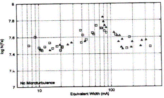
Figure 4.1: log N(Fe) versus Equivalent widths using zero microturbulence.

Omitting microturbulence altogether introduces a conspicuous hump in the abundance pattern; most sensitive are lines of intermediate strength with equivalent widths in the range 60- 100 mÅ. Figure 4.1 gives a clear picture of what happens if the presence of small scale motions in the stellar atmosphere is neglected in line formation calculations.

In this section we have used the Fe I line data from Blackwell, Lynas- Gray and Smith [22] to study the effect of microturbulence, while keeping the abundance fixed at the meteoritic value of 7.51. The results are shown in Table 4.1.

Table 4.1: Microturbulence Analysis of Oxford Fe I Lines. The line broadening cross -sections $\sigma$ and velocity parameters $\alpha$ were obtained by interpolation in the tables of Anstee and O’Mara [5]. The microturbulence required to match the observed equivalent widths were obtained using the spectrum synthesis program of Ross [2]. ’*’ indicates lines which are weaker (less than 60 mÅ) and as weaker lines are not affected by microturbulence we get very high values of microturbulence if we keep the abundance fixed at 7.51.

Wavelength	Equivalent	Broadening	Enhance-	Velocity	Microturbulence
(Å)	Width	Cross-	ment	Parameter	($\xi$ km/s) with
	(mÅ)	section $\sigma$	Factor	$\alpha$	an abundance
		(a${}^{2}_{0}$)			7.51
4389.24	71.70	218	2.13	0.250	1.010
4445.47	38.80	219	2.15	0.250	2.300*
5247.06	65.80	206	3.30	0.254	1.220
5250.21	64.90	208	3.22	0.254	1.240
5701.55	85.10	364	2.05	0.241	1.110
5956.70	50.80	229	2.54	0.252	1.695
6082.71	34.00	240	1.99	0.249	2.170*
6137.00	63.80	282	1.62	0.266	0.952
6151.62	48.20	280	1.62	0.264	1.148
6173.34	67.40	283	1.62	0.267	1.025
6200.32	75.60	354	2.20	0.240	1.148
6219.29	91.50	280	1.63	0.264	0.940
6265.14	86.80	277	1.63	0.262	1.065
6280.63	62.40	225	2.85	0.253	1.305
6297.80	75.30	280	1.63	0.264	1.012
6322.69	79.20	348	2.25	0.242	1.316
6481.88	64.20	312	2.47	0.246	1.311
6498.95	44.30	228	2.93	0.254	2.500*
6574.24	26.50	229	2.96	0.254	9.000*
6593.88	86.40	324	2.43	0.248	1.154
6609.12	65.50	337	2.37	0.246	1.267
6625.04	13.60	230	2.98	0.254	13.00*
6750.15	75.80	282	NA	0.260	1.132
6945.21	83.80	279	NA	0.261	1.076
6978.86	80.10	283	NA	0.261	1.102
7723.20	38.50	255	NA	0.260	5.300*

As stated by Holweger [21] and described above, the lines most affected by microturbulence are lines of intermediate strengths between 60- 100 mÅ, hence we have omitted weaker lines in our analysis. The variation of microturbulence for equivalent widths in range of 60- 100 mÅ is between 0.9 to 1.3 km/s. The mean value is 1.14 $\pm$ 0.12 km/s.

4.3 Conclusions

Using the lines most sensitive to microturbulence with equivalent widths in the range of 60- 100 mÅ it has been shown that a microturbulence of 1.14 $\pm$ 0.12 km/s is required if these lines are to yield the same abundance of iron as that obtained by Anstee, O’Mara & Ross [9] and in meteorites. This value is somewhat larger than 1.0 km/s, a value commonly employed in analysis of the solar spectrum. As $\alpha$ Cen A is very similar to the Sun, and as a similar method will be used to determine the microturbulence in $\alpha$ Cen A, this new value 1.14 km/s will be a useful benchmark for comparison.

Chapter 5 Data Analysis for $\alpha$ Cen A

5.1 $\alpha$ Cen – the Closest Stellar System

$\alpha$ Cen is of special interest as it is the closest stellar system to the Sun. $\alpha$ Cen lies 4.35 light- years from the Sun. It is not a single star but is actually a triple star system. Its brightest and warmest star is called $\alpha$ Cen A. It is a yellow star with spectral type of G2, exactly the same as that of the Sun. Therefore its temperature ($\sim$ 5800 K) and color are similar to those of the Sun. $\alpha$ Cen A, the brightest star in the system, is slightly more massive and luminous, its mass is 1.09 solar masses and its brightness is 54 percent greater than that of the Sun.

$\alpha$ Cen B, the second brightest star in the system, lies close to $\alpha$ Cen A. It is an orange star, cooler and smaller than the Sun. Its spectral type is K1 and its surface temperature is 5300 K, approximately 500 K lower than that of the Sun. The mass of $\alpha$ Cen B is 0.90 solar masses and this star’s brightness is just 44 percent of the solar value. The brightest components $\alpha$ Cen A and B form a binary. They orbit each other in about 80 years with a mean separation of 23 astronomical units. Figure 5.1 shows the comparative size of $\alpha$ Cen stars with the Sun, taken from Croswell [6].

The third and the faintest member of the $\alpha$ Cen system, $\alpha$ Cen C, lies a long way

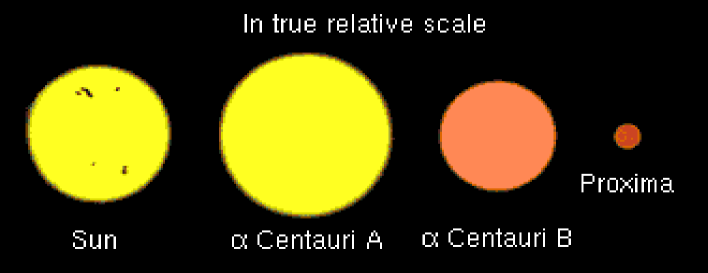
Figure 5.1: Relative Size of $\alpha$ Cen Stars compared to the Sun.

from its two brighter companions. $\alpha$ Cen C lies 13,000 AU from A and B, or 400 times the distance between the Sun and Neptune. It is not yet known whether $\alpha$ Cen C is really bound to A and B, or whether it has left the system some million of years ago. $\alpha$ Cen C lies measurably closer to the Sun than the other two: it is only 4.22 light- years away, and it is the nearest individual star to the Sun. Because of its proximity, $\alpha$ Cen C is also called Proxima Cen. Proxima Cen is a dim red dwarf, much fainter, cooler and smaller than the Sun. Its spectral type is M5, temperature is half that of the Sun, mass one- tenth that of the Sun, and brightness a mere 0.006 percent that of the Sun [6]. Proxima is so faint that astronomers did not discover it until 1915.

5.2 Observation and Data

The analysis of $\alpha$ Cen A reported here is differential to the Sun and based on an entirely new set of observational data. The observational material for $\alpha$ Cen A consists of high resolution, high $S/N$ ratio spectra obtained at Mt. Stromlo and Siding Spring Observatories (MSSSO), and the solar data are from the Kitt Peak solar flux atlas of Kurucz et al. [23].

Table 5.1: Comparison of the Sun with $\alpha$ Cen Stars [6].

The Sun and its	Sun	$\alpha$ Cen A	$\alpha$ Cen B	Proxima
Nearest
Neighbours
Color	Yellow	Yellow	Orange	Red
Spectral Type	G2	G2	K1	M5
Temperature	5770 K	5800 K	5300 K	2700 K
Mass	1.00	1.09	0.90	0.1
Radius	1.00	1.2	0.8	0.2
Brightness	1.00	1.54	0.44	0.00006
Distance (light years)	0.00	4.35	4.35	4.22
Age (billion years)	4.6	5- 6	5- 6	1?

Spectral data for $\alpha$ Cen A were taken by Dr. Mike Bessell at MSSSO. The spectra were taken on the 74 inch telescope at Mt. Stromlo Observatory in June and July 1996 with the echellé system. They were taken with the 120 inch focal length coudé camera and a 31.6 groove/mm echellé cross dispersed with a 150 lines/mm grating. The CCD was a SITe 2048x2048 CCD with 24 micron pixels. A fast rotating B star was also observed for the red settings so that the atmospheric absorption lines due to water and $O_{2}$ could be identified and removed. The $S/N$ varied with order across the CCD because of the vignetting due to the cross- disperser not being near a pupil. The actual resolution was about 3 pixels (these 1024 ”pixels” were double binned pixels of the 2048 CCD pixels) leading to an effective resolving power of about 200,000. The CCD had a gain of 2 electrons per ADU so most of the exposures were aimed at about 60000 electrons maximum. As the data were between 60000 and 180000 electrons per resolution element, the nominal $S/N$ ratio was between 200 to 400.

Around 100 spectral frames of $\alpha$ Cen A with very high resolution were obtained, giving almost continuous coverage from 4000–7000 Å. These data were used for the $\alpha$ Cen A analysis.

The data were sent in two forms. One was formatted FITS files and second was in a hard copy plot of the data. Unfortunately, the FITS files became unusable because of errors in the transmission and hence ASCII files were used directly for data analysis. The spectral frames were in blocks of nearly 16- 20 Å and strong lines were used to identify their wavelengths. A detailed analysis (formatting) of data was carried out to make data usable for the spectral line synthesis program (SYN) developed by John Ross [2]. The following sections describe how the procedure was carried out and what modifications were required in the programs.

5.3 Spectrum Synthesis Program (SYN)

The Spectrum Synthesis program (SYN) developed by John Ross [2], is an adaptation of a program first used by Ross & Aller (1976) [24]. The synthesis program, which runs on an IBM- compatible PC with an 80486 DX processor and VGA graphics, is highly interactive. The observed and computed spectra with the residual error multiplied by a factor of 5 are displayed simultaneously. Parameters such as the collisional damping constant, the abundance, the line wavelength, continuum level and so on, can be changed at will to minimize the residual error. In addition, blending lines can be added to the spectra in cases where they affect the fitting process. The software is now accessible over the Internet [2].

5.4 Identification of Spectral Lines

Identification of lines was carried out using the solar spectrum identification list of Moore et al. [7] because $\alpha$ Cen A is similar to the Sun in composition as well as effective temperature. Using the line identification list, the hard copy of the spectrum of $\alpha$ Cen A, and the solar flux atlas displayed on a computer it was easy to identify individual lines in $\alpha$ Cen A.

$\alpha$ Cen A spectra were in spectral frames of approximately 20 Å and it was not continuous. The spectral data was basically in the range of 3700 Å to 6000 Å and one additional separate range of 7000 Å to 8000 Å was also available. Identifying major lines of Fe (iron), Mg (magnesium), Ca (calcium), etc., was done and a table similar to the solar atlas was made ($\alpha$ Cen atlas).

5.5 Data Formatting for SYN

The ASCII data files contained intensity values corresponding to channel numbers. Each file had 1024 data points and had a wavelength range of about 20 Å. A cubic least squares fitting process was used to obtain the relationship between channel numbers and the wavelengths of identified lines (a process popularly known as scrunching the spectrum). The values obtained were used in a FORTRAN program to generate data files having intensity values corresponding to the wavelengths. The data files with intensity and wavelengths had irregular wavelength intervals. The data files were interpolated using MATLAB to a uniform wavelength interval of 0.01 Å. Each data set was then scaled so that the highest point in the continuum was 9999, the value used in the spectrum synthesis program. Data files were merged to form 100 Å blocks, so, the file contained data from wavelength 3700.00 Å to 3799.99 Å, 3800.00 Å to 3899.99 Å and so on. Finally these data files were converted from ASCII to binary, the format required by the synthesis program SYN.

The $\alpha$ Cen A spectrum was compared with the solar flux spectrum in the ATLAS program (a program originally developed by J. E. Ross to compare different atlases of the solar spectrum). During this comparison some spectral frames of $\alpha$ Cen A showed a ’tilt’ towards either of the blue or red side of the spectrum. The ATLAS program was modified to allow these tilts to be removed. The ATLAS program also provides the facility to shift the spectrum both horizontally (wavelength) and vertically (intensity) to help in straightening the spectra.

The above mentioned process and programming were carried out to satisfy the requirements of the SYN program. The SYN program uses these binary files to plot the observed spectrum. It also uses data files which contain parameters from the chosen atmospheric model and atomic data for the lines to compute the theoretical spectrum. The program then compares the observed and the theoretical spectra to deduce the abundance of a particular element.

SYN requires an accurate atmospheric model for the comparison of the theoretical spectrum and the observed spectrum. SYN contains a program for computing a model atmosphere using as input data, the assumed temperature distribution, surface gravity and composition. As the effective temperature of $\alpha$ Cen A is close to that of the Sun, the temperature distribution can be obtained by scaling the temperature distribution of a solar model to the effective temperature distribution of $\alpha$ Cen A. The Holweger- Müller model [25] for the Sun was used for this purpose.

Chapter 6 Results and Discussion

6.1 Importance of Strong Lines in Determining Chemical Composition

Weak, medium- strong, and very strong lines can be used to determine the chemical composition of a star. Weak lines have the advantage that their equivalent widths are independent of all forms of broadening. However, because they are faint it is difficult to measure their intrinsic strengths in the laboratory with any precision and to observe them with sufficient $S/N$ ratio in all stars other than the Sun. Also they are very susceptible to the presence of weak unknown blends.

Medium- strong lines having equivalent widths of about 80 mÅ present their own problems. As pointed out by Holweger [21], the abundance derived from such lines is particularly sensitive to non- thermal motions (microturbulence) in the stellar photosphere. This sensitivity is largely responsible for the disparity between determinations of the abundance of iron in the Sun by different groups.

Finally, the method which is used here and the method which is capable of estimating abundances to quite a degree of accuracy, is the use of very strong lines with well developed damping wings for abundance determination. The problem which weak lines face is solved here, as the strengths of these strong lines in laboratory sources makes it easier to determine their f- values with some precision. The problem of non- thermal motions is solved by the process of fitting the wings of these lines, which excludes the line core, which is affected by non- thermal motions of the atoms and is more sensitive to the deviations from the local thermodynamic equilibrium (LTE).

The major problem of using these strong lines for abundance determination in the past was the lack of suitable empirical or theoretical damping constants. Now, with the use of the tables of line- broadening cross- sections produced by Anstee & O’Mara [5] for s- p and p- s transitions, it is possible to obtain damping constants. Anstee & O’Mara [5] and Anstee, O’Mara & Ross [9] have shown that these damping constants with good f- values for a selection of strong lines produce solar abundances that are consistent with meteoritic abundances.

This method and these damping constants are used here to determine the abundance of selected elements in $\alpha$ Cen A, a solar- type star.

6.2 Parameters for an Atmospheric Model

There are four parameters of importance in determining the atmospheric model for a star. They are effective temperature ($T_{e}$), surface gravity (log g), chemical composition and microturbulence ($\xi$). All four parameters, and how they are used in this analysis, are described in brief below.

6.2.1 Effective Temperature ($T_{e}$)

The effective temperature ($T_{e}$) of $\alpha$ Cen A is considered to be nearly same as that of the Sun. Its color suggests a range from the solar effective temperature of 5780 K to 5820 K. In this analysis we have used two models with different effective temperatures, one with the solar effective temperature 5780 K and the other, 5820 K, obtained by Bessell [10]. The resultant abundance of the elements obtained in these two cases should bracket the range for $\alpha$ Cen A.

6.2.2 Surface Gravity (log g)

The surface gravity (log g) is one of the most important parameters in estimating the chemical composition of $\alpha$ Cen A. Its variation has lead to differences in the exact value of the overabundance in $\alpha$ Cen A. Chmielewski et al. [3] found log g to be 4.31 $\pm$ 0.02 while Furenlid & Meylan [4] found a low value for log g of 4.0 $\pm$ 0.2. To check the value of log g, the angular diameter $86.2*10^{-4}$ arcsec from Blackwell & Shallis [12], the parallax of 0.7506” from Furenlid & Meylan [4], leads to

$$R_{\alpha CenA}=1.234R_{\odot}.$$ (6.1)

This value of the radius is in agreement with the value of 1.23$R_{\odot}$ obtained by Soderblom [14]. If the parallax is 0.754”, as obtained from Hipparcos data [26], the radius comes out to be 1.228$R_{\odot}$ which is in agreement with both the above values to within the uncertainties involved.

Using the above value of the radius, the mass of 1.085$M_{\odot}$ from Furenlid & Meylan [4] and log $g_{\odot}$ = 4.44 in the expression

$$g/g_{\odot}=(M/M_{\odot})*1/(R/R_{\odot})^{2}$$ (6.2)

we get,

$$log(g/g_{\odot})=-0.14$$ (6.3)

which gives,

$$log(g_{\alpha CenA})=4.30\pm 0.04$$ (6.4)

The estimated uncertainty of $\pm$0.04 is based on the uncertainty in the parallax and in the radius. The lower surface gravity means the number density of hydrogen atoms is less than in the Sun and hence the line broadening is reduced. This is shown to be important later where inspite of the profiles of strong lines in the spectrum of $\alpha$ Cen A being nearly the same as the Sun, a higher abundance of the element is required to make up for the reduced line broadening.

This value of surface gravity is kept fixed throughout the analysis.

6.2.3 Microturbulence ($\xi$)

Microturbulence ($\xi$) is also a very important parameter in the determination of abundances of elements in $\alpha$ Cen A. It has been stated previously, in Chapter 4, that the microturbulence is very important for lines having intermediate strengths of 60- 100 mÅ. In the first part of this analysis, strong lines of Fe, Mg, Ca and Na are used to obtain the abundance of these elements in $\alpha$ Cen A, the strong lines are not affected by microturbulence. In the second part, medium- strong lines of iron are used to determine microturbulence, by fixing the abundance of iron to the value obtained from the first part, thus leading to an independent determination of the microturbulence which can then be used in the determination of the abundance of other elements with no strong lines in the star.

6.2.4 Chemical Composition

The fourth parameter, the chemical composition, is determined from the synthesis of the strong lines. However, as the composition has an influence on the atmospheric model several iterations may be necessary before the appropriate composition and model are obtained.

6.3 Chemical Composition Using Strong Lines

6.3.1 Selection of Lines

Strong lines for determining the abundance of iron in $\alpha$ Cen A were obtained from Anstee, O’Mara & Ross [9]. The A grade lines of iron from Anstee, O’Mara & Ross [9] have good f- values and lead to an accurate abundance of iron in the Sun. Also the Mg b- lines, the Na D- lines and the Ca I resonance line were used in the analysis.

6.3.2 Atmospheric Model

Four different model configurations based on the Holweger and Müller model [25] (hereafter referred to as the HM model) for the Sun were used in this analysis. The first model was the HM model with a solar composition and log g equal to 4.3 (as calculated in section 6.2.2). In the second model the abundances obtained from the first were used to determine a new model which reflects the higher metallicity of $\alpha$ Cen A. To allow for the possibility that $\alpha$ Cen may be bluer and hotter than the Sun the temperature distribution in the second model was scaled to the effective temperature of 5820 K (third model) suggested by Bessell [10]. A fourth model was then constructed from the third to incorporate the higher abundances resulting from the increase in the effective temperature.

6.3.3 Abundance Analysis

The spectrum synthesis program (SYN) was used for obtaining abundances of the strong lines. This software enables the computed profile of the lines to be compared with the observed line profile. In the software, the abundance was adjusted so as to minimize the difference between the observed and the computed spectrum, which is displayed on the computer screen scaled up by a factor of 5. The fitting process concentrates on the damping wings of the line so that the derived abundance is independent of the macroturbulent and microturbulent velocities.

The derived abundances obtained from the selected strong lines using the first model are shown in Table 6.1. The difference in the last column is the difference between $\alpha$ Cen A and the solar abundances. The iron abundance obtained for $\alpha$ Cen A is compared with the iron abundance of the Sun obtained by Anstee, O’Mara & Ross [9]. The Mg, Na and Ca abundances for $\alpha$ Cen A are compared with observed solar abundances. For Ca, the difference of 0.14 dex is obtained by assuming a solar abundance of Ca of 6.36 obtained using a selection of lines in the Sun. A solar abundance based on only the $\lambda$4226.74 line comes out to be 6.38 and hence a lower overabundance of 0.12 dex. Table 6.2 shows the mean abundances and the mean overabundance compared to the solar abundances.

Table 6.1: Abundance Analysis from Strong Lines of $\alpha$ Cen A using the first model. The columns in order are: element, wavelength, log gf, line broadening cross- section $\sigma$, velocity exponent $\alpha$ from the tables of Anstee & O’Mara [5], reduced equivalent width from Moore et al. [7], logarithmic abundance and the difference compared to observed solar abundances. Tables 6.3 and 6.5 have similar columns.

Element	$\lambda$	log gf	$\sigma$	$\alpha$	$\Delta\lambda/\lambda$	logN/N(H)	Difference
	(Å)		(a${}^{2}_{0}$)			+12	(dex)
Fe	4071.738	-0.022	332	0.250	191	7.60	+0.10
Fe	4383.545	0.20	298	0.262	235	7.61	+0.10
Fe	4415.123	- 0.615	308	0.257	92.9	7.62	+0.10
Fe	4918.994	-0.340	750	0.237	53.7	7.64	+0.13
Fe	4957.299	-0.410	738	0.239	56.76	7.67	+0.16
Fe	4957.597	0.230	724	0.240	128	7.67	+0.16
Fe	5232.940	-0.06	724	0.241	64.9	7.64	+0.13
Fe	5269.537	-1.321	239	0.249	87	7.63	+0.12
Fe	5328.029	-1.466	241	0.249	70.4	7.63	+0.12
Fe	5328.532	-1.850	240	0.257	39.4	7.63	+0.11
Fe	5371.490	-1.645	242	0.249	44.1	7.66	+0.14
Fe	5446.917	-1.86	243	0.249	42.8	7.62	+0.11
Mg	5167.327	-0.857	731	0.240	173	7.68	+0.10
Mg	5172.698	-0.380	731	0.240	234	7.68	+0.10
Mg	5183.619	-0.158	731	0.240	303	7.69	+0.11
Mg	5528.905	-0.470	1471	311	53.8	7.69	+0.11
Ca	4226.740	0.243	372	242	342	6.50	+0.12
Na	5889.973	0.1173	409	263	120	6.41	+0.13
Na	5895.940	-0.1838	409	237	91	6.43	+0.15

Table 6.2: Mean Abundances and Mean Overabundance for $\alpha$ Cen A using the first model.

Element	Mean Logarithmic	Mean
	Abundance	Overabundance (dex)
Fe	7.63 $\pm$ 0.02	0.12 $\pm$ 0.02
Mg	7.68 $\pm$ 0.01	0.10 $\pm$ 0.01
Ca	6.50 (1 line)	0.12 (1 line)
Na	6.42 $\pm$ 0.01	0.14 $\pm$ 0.01

The atmospheric model was revised to add the higher abundance obtained for $\alpha$ Cen A. The revised model was again used to get the abundances of the strong lines. The abundances obtained using the second model are shown in Table 6.3. Table 6.4 shows the mean abundance and mean overabundance for $\alpha$ Cen A using the higher abundance in the model (the second model). Here also the iron abundance is compared with the solar iron abundance obtained by Anstee, O’Mara & Ross [9].

Table 6.3: Abundance Analysis from Strong Lines of $\alpha$ Cen A using the second model.

Element	$\lambda$	log gf	$\sigma$	$\alpha$	$\Delta\lambda/\lambda$	logN/N(H)	Difference
	(Å)		(a${}^{2}_{0}$)			+12	(dex)
Fe	4071.738	-0.022	332	0.250	191	7.62	+0.12
Fe	4383.545	0.20	298	0.262	235	7.63	+0.12
Fe	4415.123	- 0.615	308	0.257	92.9	7.64	+0.12
Fe	4918.994	- 0.340	750	0.237	53.7	7.67	+0.16
Fe	4957.299	- 0.410	738	0.239	56.76	7.71	+0.20
Fe	4957.597	0.230	724	0.240	128	7.71	+0.20
Fe	5232.940	- 0.06	724	0.241	64.9	7.67	+0.16
Fe	5269.537	- 1.321	239	0.249	87	7.65	+0.14
Fe	5328.029	-1.466	241	0.249	70.4	7.65	+0.14
Fe	5328.532	-1.850	240	0.257	39.4	7.65	+0.13
Fe	5371.490	-1.645	242	0.249	44.1	7.69	+0.17
Fe	5446.917	-1.86	243	0.249	42.8	7.64	+0.13
Mg	5167.327	-0.857	731	0.240	173	7.74	+0.16
Mg	5172.698	-0.380	731	0.240	234	7.74	+0.16
Mg	5183.619	-0.158	731	0.240	303	7.74	+0.16
Mg	5528.905	-0.470	1471	311	53.8	7.74	+0.16
Ca	4226.740	0.243	372	242	342	6.55	+0.17
Na	5889.973	0.1173	409	263	120	6.48	+0.20
Na	5895.940	-0.1838	409	237	91	6.48	+0.20

Table 6.4: Mean Abundances and Mean Overabundance for $\alpha$ Cen A using the second model.

Element	Mean Logarithmic	Mean
	Abundance	Overabundance (dex)
Fe	7.66 $\pm$ 0.03	0.15 $\pm$ 0.03
Mg	7.74 $\pm$ 0.00	0.16 $\pm$ 0.00
Ca	6.55 (1 line)	0.17 (1 line)
Na	6.48 $\pm$ 0.00	0.20 $\pm$ 0.00

The third revision of the model was done by scaling the temperatures by the ratio of an estimated effective temperature of $\alpha$ Cen A, 5820 K (from literature reviewed) to the solar effective temperature, 5780 K (used in previous models). The basis of this scaling follows from what one would expect for the case of a grey model atmosphere in which the opacity is independent of wavelength, where, the temperature distribution for $\alpha$ Cen A is given by

$$T^{4}_{\alpha CenA}(\tau)=T^{4}_{e(\alpha CenA)}*(\tau+q(\tau))$$ (6.5)

where, $\tau$ is the optical depth and q($\tau$) is a function which is chosen to make the flux independent of depth in the grey model atmosphere. The temperature distribution for the Sun is given by

$$T^{4}_{\odot}=T^{4}_{e\odot}*(\tau+q(\tau))$$ (6.6)

Taking the ratio and the fourth root, we get,

$$T_{\alpha CenA}(\tau)=(T_{e(\alpha CenA)}/T_{e\odot})*T_{\odot}(\tau)$$ (6.7)

Abundances obtained using the model with the higher effective temperature after iterating the composition to reflect the higher temperature, i.e. model 4, are shown in Table 6.5 and their average values are shown in Table 6.6.

Table 6.5: Abundance Analysis from Strong Lines of $\alpha$ Cen A using the third and the fourth model.

Element	$\lambda$	log gf	$\sigma$	$\alpha$	$\Delta\lambda/\lambda$	logN/N(H)	Difference
	(Å)		(a${}^{2}_{0}$)			+12	(dex)
Fe	4071.738	- 0.022	332	0.250	191	7.67	+0.17
Fe	4383.545	0.20	298	0.262	235	7.70	+0.19
Fe	4415.123	- 0.615	308	0.257	92.9	7.70	+0.18
Fe	4918.994	- 0.340	750	0.237	53.7	7.74	+0.22
Fe	4957.299	-0.410	738	0.239	56.76	7.77	+0.26
Fe	4957.597	0.230	724	0.240	128	7.77	+0.26
Fe	5232.940	-0.06	724	0.241	64.9	7.70	+0.19
Fe	5269.537	-1.321	239	0.249	87	7.69	+0.18
Fe	5328.029	-1.466	241	0.249	70.4	7.70	+0.19
Fe	5328.532	-1.850	240	0.257	39.4	7.71	+0.19
Fe	5371.490	-1.645	242	0.249	44.1	7.72	+0.20
Fe	5446.917	-1.86	243	0.249	42.8	7.69	+0.18
Mg	5167.327	-0.857	731	0.240	173	7.78	+0.20
Mg	5172.698	-0.380	731	0.240	234	7.79	+0.21
Mg	5183.619	-0.158	731	0.240	303	7.80	+0.22
Mg	5528.905	-0.470	1471	311	53.8	7.78	+0.20
Ca	4226.740	0.243	372	242	342	6.59	+0.21
Na	5889.973	0.1173	409	263	120	6.53	+0.25
Na	5895.940	-0.1838	409	237	91	6.53	+0.25

Table 6.6: Mean Abundances and Mean Overabundance for $\alpha$ Cen A using the third and the fourth model.

Element	Mean Logarithmic	Mean
	Abundance	Overabundance (dex)
Fe	7.71 $\pm$ 0.03	0.20 $\pm$ 0.03
Mg	7.79 $\pm$ 0.01	0.21 $\pm$ 0.01
Ca	6.59 (1 line)	0.21 (1 line)
Na	6.53 $\pm$ 0.00	0.25 $\pm$ 0.00

Figures 6.1, 6.2 and 6.3 are self explanatory. The observed line profile is shown by a solid line and the computed line profile is represented by dots. Figure 6.1 shows the $\lambda$4226.74 resonance line of neutral calcium. This very strong line, synthesised with numerous blending lines, give a quite accurate calcium abundance. As only this line is used, the abundance comparison and hence the overabundance is calculated with respect to this line only. The second plot shows the $\lambda$5895.94 sodium ($D_{2}$) line. Due to the fact that Mt. Stromlo is neither high nor dry the wings suffer from considerable contamination by telluric water vapour lines causing uncertainty in determination of the overabundance.

Figure 6.2 shows how the process of determining abundance by strong lines is important using spectrum synthesis. The first plot gives the best fit to the $\lambda$5269.53 iron line. The neighbouring line is a medium- strong calcium line. The second plot shows the variation in the wings of this line when abundance is changed by $\pm$0.1 dex. Matching the wings of this line results in an abundance independent of microturbulence.

Figure 6.3 shows the $\lambda$5172.69 magnesium b- line. It also shows the neighbouring medium- strong lines of iron. The second plot shows $\lambda$5328.02 and $\lambda$5328.53 pair of iron lines.

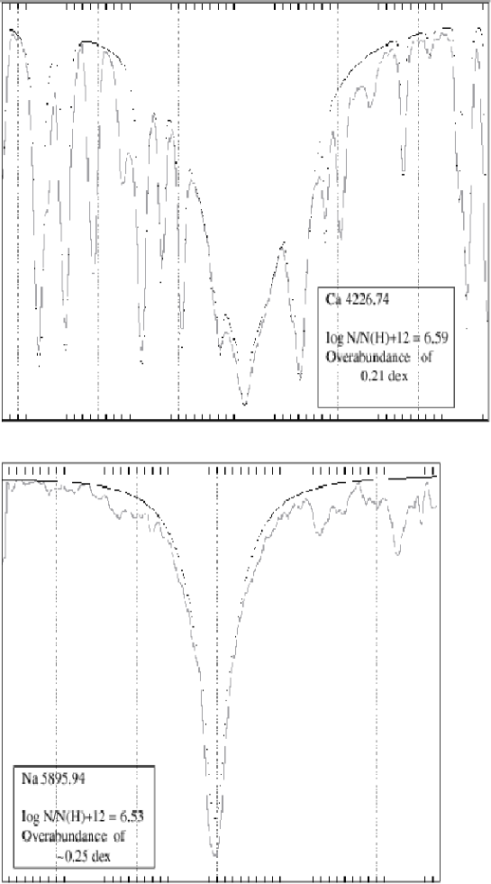
Figure 6.1: Resonance line of neutral calcium $\lambda$4226.74 (top) and Sodium ($D_{2}$) line $\lambda$5895.94 (bottom). The vertical scale is the residual intensity with a residual intensity of zero at the bottom of each plot and unity just below the top of the plots. The horizontal scale is the wavelength, with the angström markers extending from the top to the bottom of the plots with one- tenth angström markers in between. Figures 6.2 and 6.3 have similar vertical and horizontal scales.

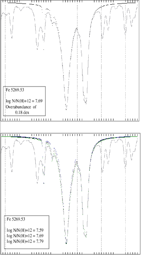
Figure 6.2: The upper plot shows the observed profile (line) for the $\lambda$5269.53 line and the computed profile (dots) that best fits the observed line profile. The lower plot shows the fit for an abundance 0.1 dex lower and 0.1 dex higher than the abundance that best fits the line profile. This lower plot clearly identifies the damping wings of the line and the core, which is dominated by photospheric motions.

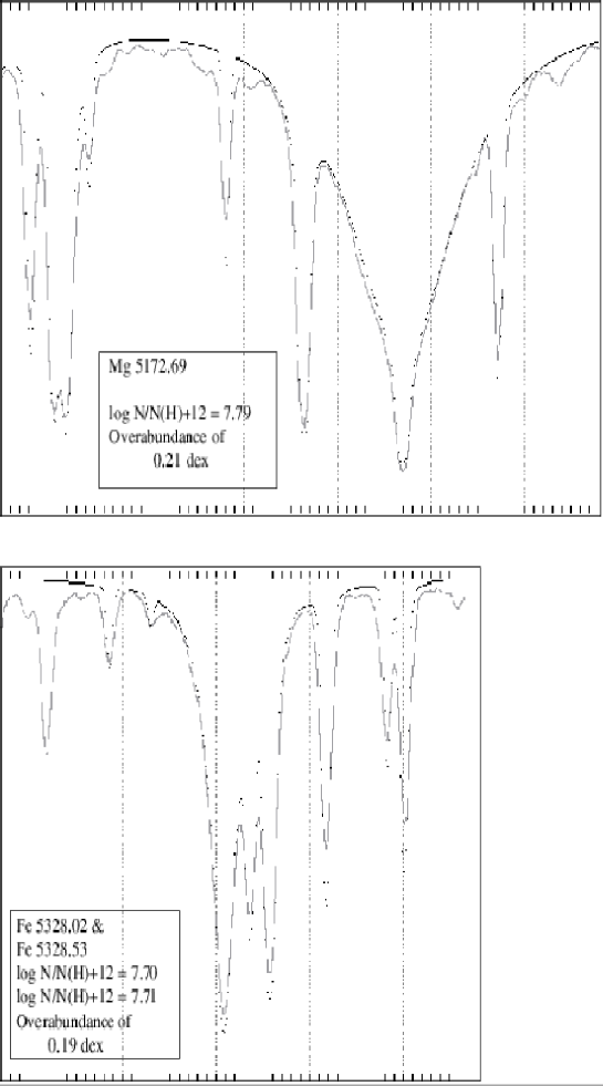
Figure 6.3: Magnesium b- line $\lambda$5172.69 (top) and Iron lines $\lambda$5328.02 and $\lambda$5328.53 (bottom)

The results obtained for $\alpha$ Cen A in Table 6.6 are the final results for its chemical analysis. The results clearly show that $\alpha$ Cen A is a metal rich star compared to the Sun. A few important points to be noted from this analysis are as follows:

• The abundance of metals other than iron are obtained using the wings of very few lines. The Mg abundance obtained from four strong lines of magnesium is quite accurate, the Ca abundance could be obtained from the only strong line available, and the Na abundance obtained from two strong lines is likely to be overestimated because of presence of water vapour lines in the wings of these two lines as shown in Figure 6.1.

• The effect of temperature on iron lines was noticeable, raising the temperature raises the computed abundance, with some lines more affected than others. The increase in the derived abundance was particularly noticeable for the iron line pair of $\lambda$4957.29 and $\lambda$4957.59.

• The value of log g is known with an accuracy of at least 10% and therefore should not, as was the case in the analysis of Furenlid & Meylan [4], be regarded as an adjustable parameter in the analysis. The only problem in the model seems to be the value of the effective temperature. When medium- strong lines are used in an extension of this analysis one could use variations in the abundance of an element with excitation potential to aid in the determination of the most suitable effective temperature.

6.4 The Determination of the Microturbulence from Medium–Strong Lines of Iron in $\alpha$ Cen A

6.4.1 Selection of Lines

Medium–strong lines having equivalent widths in the range of about 60–100 mÅ were used for estimating the microturbulence in $\alpha$ Cen A. The lines of Blackwell et al. [22], which were used in Chapter 4 for solar microturbulence, are used here for $\alpha$ Cen A. The equivalent widths for most of the lines were available from Furenlid & Meylan [4], while some of the lines were used from our own data, approximating the equivalent widths by fitting computed and observed lines in the spectrum synthesis program. Few lines which were not in the Furenlid & Meylan [4] data and in our own data, were omitted in this analysis.

6.4.2 Microturbulence from Medium–Strong Lines of Iron

The first analysis was done using the model of Holweger Müller [25] of the Sun with log g = 4.3 and an abundance higher by 0.15 dex (the second model). Keeping the abundance fixed at 7.66 for all medium- strong lines, the equivalent width was adjusted to match the observed equivalent width by varying the microturbulence. The process was done using the SYN program of John Ross [2]. Table 6.7 shows the microturbulence obtained using this process. The line broadening cross sections ($\sigma$) and velocity parameters ($\alpha$) were obtained by interpolation in the tables of Anstee & O’Mara [5]. The mean value of microturbulence obtained from this analysis is 1.35 $\pm$ 0.13 km/s.

The process was repeated using the atmospheric model with higher effective temperature and incorporated higher abundance (the fourth model). Table 6.8 shows the microturbulence obtained using higher effective temperature and hence the higher abundance of 7.71 (0.20 dex higher). The effect of the temperature is clearly visible from this part of the analysis. As the temperature increases, the abundance from strong lines increases and consequently the microturbulence from medium–strong lines decreases. The mean microturbulence obtained with higher temperature and higher abundance is 1.34 $\pm$ 0.13 km/s.

Table 6.7: Microturbulence Analysis of Fe I Lines in $\alpha$ Cen A using the second model. The line broadening cross- sections $\sigma$ and velocity parameters $\alpha$ were obtained by interpolation in the tables of Anstee and O’Mara [5]. The microturbulence required to match the observed equivalent widths were obtained using the spectrum synthesis program of Ross [2]. ’*’ are equivalent widths estimated from the available data. The values are crudely approximated by fitting the computed spectrum to the observed spectrum. Other equivalent widths are taken from Furenlid & Meylan [4]. Table 6.8 has similar columns.

Wavelength	Equivalent	Broadening	Enhance-	Velocity	Microturbulence
(Å)	Width	Cross-	ment	Parameter	($\xi$ km/s) with
	(mÅ)	section $\sigma$	Factor	$\alpha$	an abundance
		(a${}^{2}_{0}$)			7.66
4389.24	82.00*	218	2.13	0.250	1.212
5247.06	74.00*	206	3.30	0.254	1.266
5250.21	73.00*	208	3.22	0.254	1.311
5701.55	96.00*	364	2.05	0.241	1.325
5956.70	56.00	229	2.54	0.252	1.205
6151.62	59.00	280	1.62	0.264	1.385
6173.34	75.00	283	1.62	0.267	1.175
6200.32	83.00	354	2.20	0.240	1.379
6265.14	101.00	277	1.63	0.262	1.479
6297.80	86.00	280	1.63	0.264	1.322
6593.88	101.00	324	2.43	0.248	1.596
6609.12	77.00	337	2.37	0.246	1.572
6750.15	85.00	282	NA	0.260	1.361

Table 6.8: Microturbulence Analysis of Fe I Lines in $\alpha$ Cen A using the fourth model.

Wavelength	Equivalent	Broadening	Enhance-	Velocity	Microturbulence
(Å)	Width	Cross-	ment	Parameter	($\xi$ km/s) with
	(mÅ)	section $\sigma$	Factor	$\alpha$	an abundance
		(a${}^{2}_{0}$)			7.71
4389.24	82.00*	218	2.13	0.250	1.225
5247.06	74.00*	206	3.30	0.254	1.278
5250.21	73.00*	208	3.22	0.254	1.320
5701.55	96.00*	364	2.05	0.241	1.315
5956.70	56.00	229	2.54	0.252	1.199
6151.62	59.00	280	1.62	0.264	1.346
6173.34	75.00	283	1.62	0.267	1.160
6200.32	83.00	354	2.20	0.240	1.360
6265.14	101.00	277	1.63	0.262	1.474
6297.80	86.00	280	1.63	0.264	1.312
6593.88	101.00	324	2.43	0.248	1.586
6609.12	77.00	337	2.37	0.246	1.542
6750.15	85.00	282	NA	0.260	1.346

Chapter 7 Conclusions

The abundances of iron, magnesium, calcium and sodium in $\alpha$ Cen A have been determined from strong lines and are approximately 0.2 dex higher than in the Sun. As these derived abundances are independent of non- thermal motions in the atmosphere of $\alpha$ Cen A, the metal rich status of this star is unambiguous since the higher abundances derived cannot be reduced to solar values by adopting a higher microturbulence.

The microturbulence obtained from medium- strong lines using the abundance obtained from the strong lines is 1.34 $\pm$ 0.12 km/s, i.e., 0.20 km/s larger than in the Sun, which is fully consistent with the lower surface gravity of $\alpha$ Cen A. This analysis gives a strong hold on the microturbulence making it possible to derive improved abundances of other elements for which there are no strong lines.

Future work should include:

• extension of the abundance determination to other elements,

• acquisition of the spectrum in the region from 6000 to 7000 Å, which will provide access to additional strong lines of calcium and other elements,

• better determination of the angular diameter from measurements made by the Sydney University Stellar Interferometer (SUSI) leading to a better determination of the surface gravity, and

• also spectro- photometry would lead to a better determination of the effective temperature.

Combined with even higher $S/N$ data, it should be possible to obtain excellent abundances for $\alpha$ Cen A. Assuming that the metal abundance for $\alpha$ Cen B is the same as for $\alpha$ Cen A, it should be possible to learn a great deal about stars somewhat cooler than the Sun from a similar analysis of $\alpha$ Cen B.

In summary, for the first time, an unambiguous microturbulence and metallicity for $\alpha$ Cen A has been obtained !

Appendix

$\alpha$ Cen - a Candidate for Terrestrial Planets and Intelligent Life

While this is outside the general thrust of the thesis, it may be of interest to note other reasons why the $\alpha$ Cen system has received so much attention.

Why $\alpha$ Cen is Special?

The nature of the star around which a planet orbits is an important factor in determining whether life is possible on the planet. Seventy percent of all stars in the Galaxy are red dwarfs like Proxima Cen, too faint, too cool and in some cases too variable to support life. About 15 percent are orange K- type dwarfs. Although the more luminous K dwarfs like $\alpha$ Cen B, may be bright and warm enough for life but the fainter ones in the class may be too dim and cool. Another 10 percent of stars are white dwarfs - dying stars that either could not have life, or must have destroyed any life they once had. That leaves the brightest 5 percent of all stars in the Galaxy, a privileged group to which both the Sun and $\alpha$ Cen A belong. Most of this upper 5 percent consists of yellow G- type stars that are bright, warm, and good for life.

Hence it is very important to study these type of stars as they might have intelligent life around them.

Tests for Possibility of Life

A star must pass five tests before it becomes a promising place for existence of life [8]. They are :

• The star should be on the main sequence to ensure maturity and stability.

• Spectral type of the star.

• A system must demonstrate stable conditions.

• The star’s age - a star must be old enough to give life a chance to evolve.

• Chemical composition of the star - does the star have the heavy elements that biological life needs ?

The first criterion is to ensure the star’s maturity and stability, which means it has to be on the main sequence. Main sequence stars fuse hydrogen into helium in their cores, generating light and heat. Because hydrogen is so abundant in stars, most of them stay on the main sequence a long time, giving life a chance to evolve. The Sun and all three components of $\alpha$ Cen pass this test.

The second test is much tougher. The star must have the right spectral type because this determines how much energy a star emits. The hotter stars those with spectral types O, B, A, and early F are no good because they burn out fast and die quickly, emitting ultra–violet rays. The cooler stars those with spectral types M and late K may not produce enough energy to sustain life, for instance they may not permit the existence of liquid water on their planets. Between the stars that are too hot and those that are too cool, yellow G type stars like the Sun can give rise to life. $\alpha$ Cen A passes this test as it is of the same class as our Sun. $\alpha$ Cen B is a K1 star, so it is hotter and brighter than most K stars, therefore it may pass this test or it may not. The red dwarf Proxima fails this test.

For the third test, a system must demonstrate stable conditions, as $\alpha$ Cen A and B form a binary pair how much does the light received by the planets of one star vary as the other star revolves around it? During their 80- year orbit, the separation between A and B changes from 11 AU to 35 AU. As viewed from the planets of one star, the brightness of the other increases as the stars approach and decrease as the stars recede. Fortunately, the variation is too small to matter, and $\alpha$ Cen A and B pass this test. Proxima being a red dwarf, which emits flares that causes its light to double or triple in just few minutes, fails this test.

The fourth condition concerns the star’s age. The Sun is about 4.6 billion years old, so life on earth had enough time to evolve. A star must be old enough to give life a chance to evolve. Remarkably, $\alpha$ Cen A & B are probably even older than the Sun, they have an age of about 5 to 6 billion years, therefore they pass this test, but the study of Proxima shows it to be younger compared to $\alpha$ Cen A and B, so it fails this test, too.

And the fifth and final test: Do the stars have enough heavy elements such as carbon, nitrogen, oxygen and iron, to support biological life? Like most stars, the Sun is primarily hydrogen and helium, but 2 percent of the Sun’s mass is metals. Although 2 percent may not sound a lot, it is enough to build rocky planets and to give rise to us. And again, fortunately, $\alpha$ Cen A and B pass this test. They are metal- rich stars.

Thus we see that $\alpha$ Cen A passes all five tests, $\alpha$ Cen B passes all but one, and only Proxima Cen could not satisfy most. The details are summarised in the given Table A.1.

Table A.1: Terrestrial Life Conditions Important Questions [6].

Terrestrial Life Conditions:	Sun	$\alpha$ Cen A	$\alpha$ Cen B	Proxima
Questions for Any Star
On the main sequence?	Yes	Yes	Yes	Yes
Of the right spectral type?	Yes	Yes	Maybe	No
Constant in brightness?	Yes	Yes	Yes	No
Old enough?	Yes	Yes	Yes	No?
Rich in metals?	Yes	Yes	Yes	?
Has stable planetary orbits?	Yes	Yes	Yes	Yes
Could planets form?	Yes	?	?	?
Do planets actually exist?	Yes	?	?	?
Small rocky planets possible?	Yes	Yes	Yes	Yes?
Planets in the life zone?	Yes	Maybe	Maybe	No

As stars of $\alpha$ Cen, specially $\alpha$ Cen A and B, are very similar to the Sun and probably have the same age as the Sun, the most likely question could be, Is there any possibility of an earth- like planet revolving around $\alpha$ Cen in stable orbit? The possible interpretation given by Soderblom [27] in favour of $\alpha$ Cen A goes something like this:

Three body systems are unstable unless two of the bodies are close together and the third is a large distance away. If the separation of the three are comparable, it doesn’t take long for two of them to pass close to each other, which sends at least one of them streaking off into the void, no longer bound to the other two bodies.

The distance between $\alpha$ Cen A and B varies from about 11 to 35 AU over the course of its 80 year orbit. An earth–like planet 1 AU from $\alpha$ Cen A could probably stay there indefinitely without fear of harm from $\alpha$ Cen B. According to Soderblom [27] the only question is whether an earth- like planet could form in the first place at that location. Probabilistic discussion of whether planets like earth revolve round the $\alpha$ Cen A or B is given by Croswell [6]. At the end of his discussion, Croswell [6]

Figure A.1: Possibility of Planet in Life Zone of $\alpha$ Cen [8].

concludes that it is frustrating that we can’t reach any definite conclusion. Though we can say with certainty that at least one of its star is ideal, we can say very little about any planets there. On the positive side, earth- like planets can have stable, earth- like orbits around either A or B. What is lacking is any direct evidence that such planets exist.

$\alpha$ Centauri is therefore very special; special not only for its proximity but also for its promise. If $\alpha$ Cen has planets, it is even more special since one or more of those planets could resemble Earth. So if we ever launch missions to other stars in the Galaxy, $\alpha$ Cen will certainly be our first target.

Bibliography

[1] S. D. Anstee and B. J. O’Mara. An investigation of Brueckner’s theory of line broadening with application to the sodium D lines. Monthly Notices of the Royal Astronomical Society, 253:549–560, July 1991.

[2] J. E. Ross. Homepage for spectrum synthesis program (SYN).
Web Site – http://www.physics.uq.edu.au/people/ross/syn.htm

[3] Y. Chmielewski, E. Friel, G. Cayrel de Strobel, and C. Bentolila. The 1992 detailed analyses of $\alpha$ Centauri A and $\alpha$ Centauri B. Astronomy and Astrophysics, 263:219–231, May 1992.

[4] I. Furenlid and T. Meylan. An abundance analysis of $\alpha$ Centauri A. The Astrophysical Journal, 350:827–838, February 1990.

[5] S. D. Anstee and B. J. O’Mara. Width cross sections for collisional broadening of s- p and p- s transitions by atomic hydrogen. Monthly Notices of the Royal Astronomical Society, 276:859–866, April 1995.

[6] K. Croswell. Does alpha Centauri have intelligent life? Astronomy, 19(4):28–37, 1991.

[7] C. E. Moore, M. G. J. Minnaert, and J. Houtgast. The Solar Spectrum 2935 Å to 8770 Å : Second Revision of Rowland’s Preliminary Table of Solar Spectrum Wavelengths. Washington : National Bureau of Standards, 1966.

[8] Alpha Centauri. Web Site - http://monet.physik.unibas.ch/ schatzer/Alpha Centauri.html, 1996.

[9] S. D. Anstee, B. J. O’Mara, and J. E. Ross. A determination of the solar abundance of iron from the strong lines of Fe I. Monthly Notices of the Royal Astronomical Society, 284:202–212, January 1997.

[10] M. S. Bessell. Alpha Centauri. Proceedings Astronomical Society of Australia, 4(2):212–214, 1981.

[11] V. A. French and A.L.T. Powell. Title unknown. Royal Observatory Bulletin, 173:63, 1971.

[12] D. E. Blackwell and M. J. Shallis. Stellar angular diameters from infrared photometry. Application to Arcturus and other stars; with effective temperatures. Monthly Notices of the Royal Astronomical Society, 180:177–191, February 1977.

[13] D. R. Soderblom and D. Dravins. High resolution spectroscopy of Alpha Centauri. I. Lithium depletion near one solar mass. Astronomy and Astrophysics, 140:427–430, July 1984.

[14] D. R. Soderblom. The temperatures of Alpha Centauri A and B. Astronomy and Astrophysics, 158:273–274, 1986.

[15] A. Noels, N. Grevesse, P. Magain, C. Neuforge, A. Baglin, and Y. Lebreton. Calibration of the $\alpha$ Centauri system: metallicity and age. Astronomy and Astrophysics, 247:91–94, January 1991.

[16] C. Neuforge. Alpha Centauri revisited. Astronomy and Astrophysics, 268:650–652, 1993.

[17] J. Fernandes and C. Neuforge. $\alpha$ Centauri and convection theories. Astronomy and Astrophysics, 295:678–684, 1995.

[18] S. D. Anstee, B. J. O’Mara, and J. E. Ross, editors. The Broadening of Metallic Lines in Cool Stars, January 1997.

[19] S. D. Anstee. The Collisional Broadening of Alkali Spectral Lines by Atomic Hydrogen. PhD thesis, University of Queensland, Department of Physics, 1992.

[20] P. Barklem and B. J. O’Mara. The broadening of p- d and d- p transitions by collision with neutral hydrogen atoms. Monthly Notices of the Royal Astronomical Society, 1997. Submitted.

[21] H. Holweger. Solar element abundances, Non- LTE line formation in Cool stars and Atomic data. Physica Scripta, T65:151–157, 1996.

[22] D. E. Blackwell, A. E. Lynas- Gray, and G. Smith. On the determination of the solar iron abundance using Fe I lines. Astronomy and Astrophysics, 296:217–232, 1995.

[23] R. L. Kurucz, I. Furenlid, J. Brault, and L. Testerman. The solar Flux Atlas from 296 to 1300 nm. National Solar Observatory, Sunspot, New Mexico, 1984.

[24] J. E. Ross and L. H. Aller. The chemical composition of the Sun. Science, 191:1223–1229, 1976.

[25] H. Holweger and E. A. Müller. The photospheric barium spectrum: Solar abundance and collision broadening of Ba II lines by hydrogen. Solar Physics, 39:19–30, 1974.

[26] C. Turon, D. Morin, F. Arenou, and M. A. C. Perryman. CD- ROM version of the Hipparcos Input Catalogue HICIS software. CD- ROM, 1997.

[27] D. R. Soderblom. The Alpha Centauri system. Mercury, pages 138–140, September- October 1987.