The Brera Multi-scale Wavelet HRI Cluster Survey: I Selection of the sample and number counts

We describe the construction of the Brera Multi-scale Wavelet (BMW) HRI Cluster Survey, a deep sample of serendipitous X–ray selected clusters of galaxies based on the ROSAT HRI archive. This is the first cluster catalog exploiting the high angular resolution of this instrument. Cluster candidates are selected on the basis of their X–ray extension only, a parameter which is well measured by the BMW wavelet detection algorithm. The survey includes 154 candidates over a total solid angle of $\sim$ 160 deg² at 10^-12 erg s^-1 cm^-2 and $\sim$ 80 deg² at 1.8$\times$10^-13 erg s^-1 cm^-2. At the same time, a fairly good sky coverage in the faintest flux bins ($3-5\times$10^-14 erg s^-1 cm^-2) gives this survey the capability of detecting a few clusters with $z\sim 1-1.2$, depending on evolution. We present the results of extensive Monte Carlo simulations, providing a complete statistical characterization of the survey selection function and contamination level. We also present a new estimate of the surface density of clusters of galaxies down to a flux of $3\times$10^-14 erg s^-1 cm^-2, which is consistent with previous measurements from PSPC-based samples. Several clusters with redshifts up to $z=0.92$ have already been confirmed, either by cross-correlation with existing PSPC surveys or from early results of an ongoing follow-up campaign. Overall, these results indicate that the excellent HRI PSF (5″ FWHM on axis) more than compensates for the negative effect of the higher instrumental background on the detection of high-redshift clusters. In addition, it allows us to detect compact clusters that could be lost at lower resolution, thus potentially providing an important new insight into cluster evolution.

1 Introduction

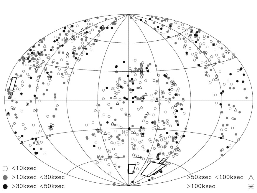
Figure 1: The spatial distribution (equatorial coordinates, Aitoff projection) of the 914 HRI pointings used for the BMW–HRI cluster survey. The origin of right ascension is in the center of the plot and the grid is in steps of $3^{h}$ in RA and $30^{\circ}$ in DEC. The empty area corresponds to the $|b_{II}|<20^{\circ}$ zone of avoidance, while the boxes mark the Magellanic clouds and Virgo cluster areas which were also excluded from the survey. Different symbols indicate different ranges of exposure time, as explained.

Clusters of galaxies represent the largest collapsed objects in the hierarchy of cosmic structures, resulting from the growth of fluctuations lying on the high–density tail of the matter density field (e.g. Peacock 1999). As such, their number density and evolution are strongly dependent on the normalization of the power spectrum and the value of the density parameter $\Omega_{M}$ (e.g. Borgani & Guzzo 2001; Rosati et al. 2002). In addition, clusters are usually considered as “simple” systems, where the physics involved in turning “mass into light” is possibly easier to understand, compared to the various complex processes connected to star formation and evolution in galaxies. In particular in the X–ray band, where clusters can be defined and recognized as single objects (not just as a mere collection of galaxies), observable quantities like X–ray luminosity $L_{X}$ and temperature $T_{X}$ show fairly tight relations with the cluster mass (e.g. Evrard et al. 1996; Allen et al. 2001; Reiprich & Böhringer 2002; Ettori et al. 2004). A full comprehension of these scaling relations requires more ingredients than a simple heating during the growth of fluctuations (Kaiser 1986; Helsdon & Ponman 2000; Finoguenov et al. 2001; Borgani et al. 2004). However, their existence and relative tightness give clusters a specific role as probes of the cosmological model, providing us with a way to test fairly directly the mass function (e.g. Böhringer et al. 2002; Pierpaoli et al. 2003) and the mass power spectrum (Schuecker et al. 2003), via respectively the observed cluster X–ray luminosity function (XLF) and clustering. In addition, and equally important, clusters at different redshifts provide homogeneous samples of essentially coeval galaxies in a high-density environment and give the possibility of studying the evolution of stellar populations (e.g. Blakeslee et al. 2003; Lidman et al. 2004).

X–ray based cluster surveys, in addition to a fairly direct connection of the observed quantities to model (mass-specific) predictions, have one further, fundamental advantage over optically-selected catalogues: their selection function is well-defined (being essentially that of a flux-limited sample) and fairly easy to reconstruct. This is a crucial feature when the goal is to use these samples for cosmological measurements that necessarily involve a precise knowledge of the sampled volume, as is the case when computing first or second moments of the density field. X–ray surveys in the “local” Universe ($\left<z\right>\sim 0.1$), stemming from the ROSAT All-Sky Survey (RASS, Voges et al. 1999) have been able to pinpoint quantities like the cluster number density to high accuracy. The REFLEX survey, in particular, has yielded the currently most accurate measurement of the XLF (Böhringer et al. 2002; 2004), in substantial agreement with other local estimates (Ebeling et al. 1997; De Grandi et al. 2001). These result provide a robust $z\sim 0$ reference frame to which surveys of distant clusters can be safely compared in search of evolution.

Recent X–ray searches for serendipitous high-redshift clusters have been based mostly on the deeper pointed images collected with the ROSAT PSPC instrument (RDCS: Rosati et al. 1995; SHARC: Collins et al. 1997; 160 Square Degrees: Vikhlinin et al. 1998a; WARPS: Perlman et al. 2002) or on the high-exposure North Ecliptic Pole area of the RASS (NEP: Gioia et al. 2003); a deeper search for massive clusters in the overall RASS is also being carried out (MACS, Ebeling et al. 2001a). Results from these surveys consistently show a lack of evolution of the XLF for $L<L^{\displaystyle\ast}_{X}\simeq 3\cdot 10^{44}$ erg s^-1 out to $z\sim 0.8$, pointing to low values of $\Omega_{M}$ under reasonable assumptions on the evolution of the $L_{X}-T_{X}$ relation (see Rosati et al. 2002 for a review). At the same time, however, they confirm the early findings from the Einstein Medium Sensitivity Survey (EMSS, Gioia et al. 1990; Henry et al. 1992) of a mild evolution of the bright end (Vikhlinin et al. 1998a; Nichol et al. 1999; Borgani et al. 2001; Gioia et al. 2001; Mullis et al. 2004). In other words, there is an indication that above $z\sim 0.6$ one finds less very massive clusters, likely indicating that beyond this epoch they were still to be assembled from the merging of smaller mass units. These conclusions, however, are still based on a rather small number of high–redshift clusters. Currently, we know $\sim 15$ X–ray confirmed clusters above $z=0.8$, with only 5 so far detected above $z=1$, all of which are at $z<1.3$. In addition, virtually all current statistical samples of distant clusters have been selected from X–ray images collected with the same, low angular resolution ROSAT-PSPC instrument. Clearly, the need for more samples of high-redshift clusters, possibly selected from independent X–ray imaging material, is compelling.

As a first contribution in this direction, during the last four years we have constructed a new sample of distant cluster candidates based on the still unexplored ROSAT-HRI archive, the BMW–HRI Cluster Survey. While serendipitous searches are already focusing on the fresh data being accumulated in the archives of the new powerful X–ray satellites XMM-Newton and Chandra (see e.g. the pioneering work by Boschin 2002), our work shows that a remarkable source of high-redshift clusters — the HRI archive — has so far been neglected. In this paper we discuss in detail the selection process, the properties of this catalogue, its completeness function and contamination. We then compute the sky coverage, number counts and expected redshift distribution of BMW–HRI clusters. The paper is organized as follows. Sect. 2 describes the general features of the HRI data and the field selection; Sect. 3 discusses the cluster detection and characterization; Sect. 4 presents the results of extensive Monte Carlo simulations, performed in order to understand the statistical properties of the cluster sample, in particular its completeness and contamination level; Sect. 5 uses all this information to derive the survey sky–coverage as a function of source flux and extension, and to compute the survey expected redshift distribution and mean surface density; Sect. 6 presents a few examples of distant clusters already identified in the BMW–HRI survey, while the last section summarizes the main results obtained in the paper.

2 Survey Description

2.1 The HRI instrument

The High-Resolution Imager (HRI) was the secondary instrument on board the ROSAT satellite, with technical features quite different from and complementary to the companion PSPC, including in particular a much better spatial resolution. The core of the HRI is a micro-channel plate detector with an octagon–like shaped field of view (with $\sim$ 19′ radius) that reveals single X–ray photons, providing information on their positions and arrival times. The HRI Point Spread Function (PSF) as measured on–axis is about 5″ FWHM, i.e. a factor of $\sim 4$ better than the PSPC . On the other hand, the HRI is less efficient than the PSPC (a factor of 3 to 8 for a plausible range of incident spectra) and has a higher background. This consists of several components: the internal background due to the residual radioactivity of the detector (1–2 cts s^-1), the externally-induced background from charged particles (1–10 cts s^-1) and the X–ray background (0.5–2 cts s^-1).

Figure 2: Distribution of exposure times for the 914 pointings used for the cluster survey.

The HRI covers the energy range [0.1–2.4] keV, divided into 16 Pulse Height Analyzer (PHA) channels, which provide very crude spectral information (Prestwich et al. 1996). The HRI background is highest in the first few (1–3) PHA channels and, at variance with the ROSAT PSPC, it is dominated by the unvignetted particle background. As shown by sky calibration sources, most of the source photons instead arrive in a PHA channel between 3 and 8 (David et al. 1998). A priori, the high background of the HRI can be a serious problem for cluster searches. The low surface brightness of these diffuse objects is indeed further suppressed as a function of redshift, due to the cosmological dimming $\propto(1+z)^{4}$ and rapidly drops below the background. Coupled to the HRI lower sensitivity, this explains why all ROSAT serendipitous cluster searches have so far concentrated on the PSPC archive (see Sect. 1). We shall show here how these early, pessimistic conclusions are fortunately not fully correct. As detailed in Campana et al. (1999, C99 hereafter), in order to minimize the background and increase the signal-to-noise (S/N) ratio of X–ray sources, especially low-surface-brightness ones, the BMW wavelet analysis has been restricted to PHA 2–9 (see also David et al. 1998). This range reduces the detector background by about 40% with a minimum loss of cosmic X–ray photons ($<10\%$; David et al. 1998). This is certainly one key feature in improving the detection of clusters of galaxies with these data, thus allowing studies to reap the benefit of the excellent resolution of this instrument.

2.2 The surveyed area

The overall BMW–HRI serendipitous catalogue (Panzera et al. 2003, P03 hereafter; Lazzati et al. 1999, L99 hereafter; C99) is based on the analysis of 4298 observations, i.e. the whole HRI archive after excluding calibration observations, fields pointed at supernova remnants and some other problematic pointings. The selection of cluster candidates imposes a number of extra selections, which are discussed here. We first selected only high Galactic latitude fields ($|b|>20^{\circ}$) with exposure times larger than 1000 seconds, excluding also the Magellanic Clouds and Virgo Cluster regions, defined in Table 1. Moreover, we excluded all pointings on star clusters, clusters and groups of galaxies and obviously Messier and NGC nearby galaxies. In all these cases the target tends to fill the field-of-view of the instrument, thus biasing any search for serendipitous sources in the surrounding area. For this reason, we further visually inspected all the remaining fields using panoramic ($40^{\prime}\times 40^{\prime}$) DSS2 images with the HRI X–ray contours overlaid, so as to ascertain whether the central target could in any way influence the searched region (as e.g. in the case of a spiral galaxy with faint arms extending out of the central 3-arcmin radius area). All fields with such “problematic” targets were excluded from the cluster candidate catalogue.

Table 1: Regions around the LMC, SMC and Virgo cluster excluded from the survey.

$$\begin{array}[]{lll}\hline\cr\vskip 3.0pt plus 1.0pt minus 1.0pt\cr{\rm region}&{\rm RA}&{\rm DEC}\\ \vskip 3.0pt plus 1.0pt minus 1.0pt\cr\hline\cr\vskip 3.0pt plus 1.0pt minus 1.0pt\cr{\rm LMC1}&[3^{h}\,52^{\prime},6^{h}\,52^{\prime}]&[-77^{\circ},-63^{\circ}]\\ {\rm LMC2}&[5^{h}\,24^{\prime},5^{h}\,56^{\prime}]&[-63^{\circ},-58^{\circ}]\\ {\rm LMC3}&[6^{h}\,52^{\prime},7^{h}\,12^{\prime}]&[-74^{\circ},-68^{\circ}]\\ {\rm SMC1}&[23^{h}\,52^{\prime},1^{h}\,20^{\prime}]&[-77^{\circ},-67.5^{\circ}]\\ {\rm SMC2}&[23^{h}\,46^{\prime},23^{h}\,54^{\prime}]&[-77^{\circ},-73^{\circ}]\\ {\rm SMC3}&[01^{h}\,20^{\prime},02^{h}\,00^{\prime}]&[-72^{\circ},-67.5^{\circ}]\\ {\rm Virgo}&[12^{h}\,20^{\prime},12^{h}\,44^{\prime}]&[7.0^{\circ},16^{\circ}]\\ \vskip 3.0pt plus 1.0pt minus 1.0pt\cr\hline\cr\end{array}$$

One further problem needing a careful treatment concerns multiple observations of the same sky areas. All these multiple pointings have been analyzed separately by the BMW–HRI general survey: consequently, the catalogue lists every source detected in each single observation, including multiple detections of the same source. To simplify the treatment of such cases, when multiple observations looked “exactly” at the same region of sky, defined as images with nominal aim points separated by less than 30″, we discarded all but the deepest exposure. However, if the separation was larger than this, we kept all the (usually overlapping) fields. The goal here was to maximize the survey area, which is the main factor in finding distant luminous clusters. These overlaps have been properly treated in the computation of the actual survey sky coverage, as explained in detail in Sect. 5.1.

Within each selected field we then considered only sources detected in the area comprised between 3′ and 15′ off–axis angle. This excludes the central part ($<$ 3′) of the field of view, which is normally where the target is pointed, and the very external part ($>$ 15′), where the sensitivity drops and the PSF worsens. We ended up with a grand total of 914 HRI observations (Fig.1) with exposure times ranging from 1 ks to 204 ks (Fig.2), for a total surveyed area of 160.4 square degrees, $\sim 7\%$ of which were observed twice or more.

3 Selection of Cluster Candidates

3.1 Source Extension Criterion

Figure 3: Source extensions as measured by the BMW detection algorithm (W_clu, see text), plotted against the off-axis angle, showing our empirical definition of extended sources. The continuous line gives the mean extension of a point–like source at different off-axis angles, and the dashed lines identifies the $3\,\sigma$ locus. Sources selected as cluster candidates have to lie, with their error bars, above the dashed line and are indicated by filled circles.

The BMW detection is based on a wavelet transform (WT) algorithm for the automatic detection and characterization of sources in X–ray images. It is fully described in L99 and has been developed to analyze ROSAT HRI images, producing the BMW–HRI catalogue (C99, P03). Candidate sources are identified as local maxima above a given threshold in wavelet space; the preliminary product of the detection procedure is a source list with a rough determination of the position (the center of the pixel with higher coefficient), source size (the scale of the WT where the signal to noise is maximized) and total number of photons (the value of the maximum WT coefficient). Since the wavelet scale steps are discrete, the final catalogue parameters are a refinement of these values and are obtained through $\chi^{2}$ minimization with respect to a Gaussian model in WT space (for all the details of the fit procedure in the WT space see L99). In particular, the BMW catalog source extension parameter (hereafter W_clu) is defined as the width of the best-fitting Gaussian.

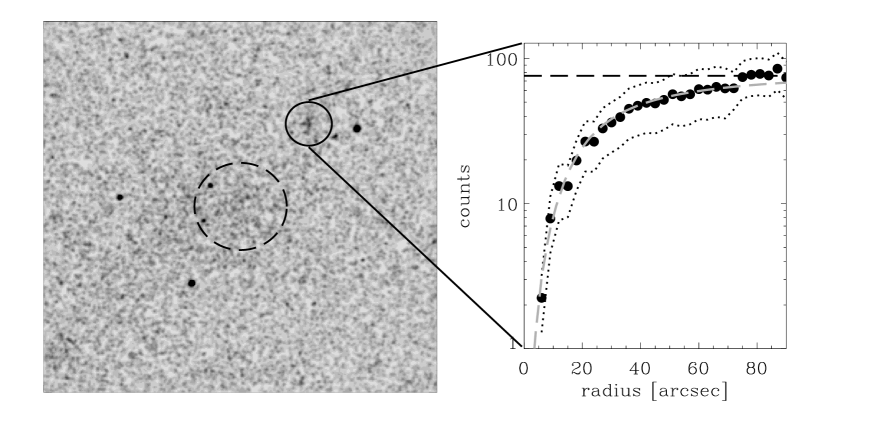
Figure 4: Left panel: $24\arcmin\times 24\arcmin$ portion of an HRI image (Gaussian smoothed with $\sigma=5\,\arcsec$) showing the detection of cluster candidate BMW044743.4-202042, marked by the solid 90″ radius circle. The dashed circle (3′ radius) indicates the central area containing the original HRI target (here barely visible), excluded from the cluster search. Right panel: Integral, background-subtracted flux growth curve of the candidate cluster (filled circles), plotted together with its 1$\,\sigma$ error corridor (dotted lines) and the best-fitting $\beta$-model (Grey dashed curve). The total flux of the source is computed as the asymptotic value of the growth curve (horizontal dashed line). From the total flux, the core radius is then derived by comparison to a grid of $\beta$ profiles convolved with the instrumental PSF at the specific off-axis angle. This is a typical source in our catalog, detected at $\sim$ 7′ off–axis with 75 net counts in a 10 ks exposure, corresponding to a flux of $\sim 3\times 10^{-13}$ erg s^-1 cm^-2.

The characterization procedure of extended sources has been explained in C99, but we briefly repeat it here for convenience of the reader. First, we considered a sub-sample of sources detected only in the observations that have a star as target (ROR number beginning with 2). This resulted in 6013 sources detected over 756 HRI fields (Fig. 3). The distribution of source extensions was divided into bins of 1′, as a function of the source off-axis angle, and within each bin, a $\sigma-$clipping algorithm on the source extension was applied: the mean and standard deviation in each bin are calculated and sources at more than $3\,\sigma$ above the mean value are discarded. In this way we determine the mean instrumental extension $\left<W_{p}(\theta)\right>$ and standard deviation $\sigma_{p}(\theta)$ of point-like source observed at different $\theta$. As shown in Fig. 3, this provides us with a threshold for defining truly extended sources (Rosati et al. 1995). We define as candidate clusters all sources that lie above the $3\,\sigma_{p}(\theta)$ corridor, including their $1\,\sigma_{clu}$ error bar, i.e. those sources for which, at their observed off-axis angle $\theta$, one has

$$W_{clu}-\sigma_{clu}>\left<W_{p}(\theta)\right>+3\,\sigma_{p}(\theta)\,\,\,\,\,.$$ (1)

This combined requirement on the distance from the point-like source locus, and on the intrinsic error in the source extension, roughly corresponds to a $\sim 3.5\,\sigma$ confidence level for the extension classification.

3.2 Significance Criterion

To reduce the contamination level of the catalogue due to spurious detections, we also limit the current cluster selection to sources with detection significance larger than $4\,\sigma$ (see Sect. 4.3). The source significance $p_{s}$ is defined as the confidence level at which a source is not a chance background fluctuation, given the background statistics and the specific field exposure time. This quantity is assessed via the signal to noise ratio in wavelet space. For each wavelet scale, the noise level is computed through numerical simulations of blank fields with the corresponding background (L99), while the signal is the peak of the wavelet coefficients corresponding to the source. In order to make this significance more easily comparable to other methods, confidence intervals are expressed in units of the standard deviation $\sigma$ for which a Gaussian distributed variable would give an equal probability of spurious detection (68%: $1\,\sigma$; 95%: $2\,\sigma$, etc.). So, the values of our figure of merit $p_{s}$ will represent the number of $\sigma$’s corresponding to the confidence level of that specific source. Note that the signal to noise in wavelet space can be different from that in direct space for several reasons: i) the background subtraction is more accurate and locally performed; ii) the high frequencies are suppressed, so that a correlated count excess gives a higher significance than a random one with the same number of counts; iii) the exposure map can be incorporated in the wavelet space, so that artifacts do not affect the source significance.

In the 914 HRI fields considered we have 194 sources meeting these requirements. Among these, we discovered that 22 were spurious sources caused by an hot pixel in the detector (not identified in the data reduction); this, coupled with the dithering of the satellite produces a high signal-to-noise extended source of 2′ typical dimension always located at the same detector coordinates.

We inspected directly each of the remaining 172 sources on DSS2/X–ray overlays and cross-correlated their positions with the NED database. As a result, we removed 18 of them from the catalog as clearly associated with a nearby galaxy, thus ending up with a final list of 154 cluster candidates. This represents our master statistical sample for follow-up. Clearly, even at $p_{s}<4\,\sigma$ a significant number of sources are truly clusters. At this level, however, the contamination rises to $\sim 40$% (see Sect. 4.3), thus making the optical identification of real clusters significantly less efficient in terms of telescope time.

3.3 Re-estimation of cluster parameters

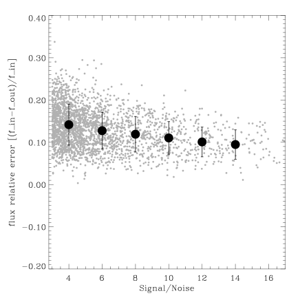
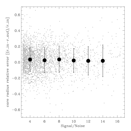
Figure 5: Relative uncertainties in the flux (left) and core radius (right) estimation, at different signal-to-noise levels, derived from the Monte Carlo simulations of the cluster sample. They are calculated as the ratio (input-output)/input. The filled circles give the mean systematic relative error in each bin and its random standard deviation.

At the end of the analysis pipeline, the BMW detection algorithm yields a catalogue with 80 parameters for each source including the count rate, flux and extension (see P03 and Sect. 3.1). These values are reliable for point sources, but not for sources with a surface brightness profile (SBP) different from the instrumental PSF, as is the case for clusters. The observed cluster profiles are the result of the convolution of the intrinsic SBP with the PSF of the instrument. The BMW algorithm calculates the source flux and extension by means of a $\chi^{2}$ minimization with respect to a Gaussian model in wavelet space (L99, see also previous section). Using a more appropriate (non–Gaussian) model within the pipeline is unpractical. First, in the general case a cluster model profile (e.g. a classical $\beta$-model or King profile, see Sect. 4) convolved with our Gaussian-based wavelet filter (L99) cannot be handled analytically, so that one of the simplifying features of the analysis pipeline is lost. Second, a direct profile fit to the data gives reliable results (in terms of $\chi^{2}$) only for the few most luminous objects in the sample, suggesting that an integral approach is the best way to proceed.

For this reason, we adopted a simple and robust “growth-curve” technique, as applied to X–ray data by Böhringer et al. (2001), to re-measure the source total flux. Fig.4 visually illustrates this technique. The source total flux is defined as the asymptotic value of the integral SBP, computed within increasing circular apertures on the background-subtracted images, when this reaches a horizontal “plateau”. The background-subtracted images are obtained from the original images by the subtraction of the background map (see Sect. 4). Technically, the plateau is defined by studying the local derivative of the growth curve, comparing at each step the flux variation within adjacent aperture radii to the expected mean error. To eliminate possible contamination from nearby sources, we first mask all other sources from the BMW–HRI general catalogue. Finally, we calculate the conversion from count–rates to fluxes assuming a bremsstrahlung spectrum with temperature $T=5$ keV and correcting for Galactic absorption using the appropriate column density at the source position (Dickey & Lockman 1990). Once the total flux of the source is established, we estimate its core radius by fitting its integral profile, adopting for the differential profile a classical $\beta$–model (Cavaliere $\&$ Fusco-Femiano 1976), with fixed $\beta=2/3$

$$I(r)=I_{0}\left[1+\left(\frac{r}{r_{c}}\right)^{2}\right]^{(-3\beta+\frac{1}{2})}=I_{0}\left[1+\left(\frac{r}{r_{c}}\right)^{2}\right]^{-{3\over 2}}\,\,\,\,,$$ (2)

where $r$ in this case describes an azimuthal quantity, with $r_{c}$ being the angular core radius. Choosing a fixed value for $\beta$ is inevitable, given the low number of photons generally characterizing our sources, which does not allow a further free fit parameter. In this way, we obtain an estimate of the source extensions. This is a very important quantity, given that, as will be clear in the following, the statistical properties of the survey strongly depend on the extension and surface brightness values of the sources. As described in the next section, we assess these properties by means of Monte Carlo simulations: in these tests we coherently assume for the input simulated clusters the fixed slope $\beta=2/3$ and variable core radii.

The actual observed SBP is then described by the convolution of the $\beta$ profile with the instrumental PSF (which depends on the off–axis position). In practice, for each cluster candidate (i.e. total flux), we compute a numerical grid of expected SBPs for different values of the core radius ranging from 2″ to 120″. We then measure the best fitting core radius by minimizing the $\chi^{2}$ between the observed and computed profiles.

The uncertainties in the measurement of these parameters are estimated via a further specific Monte-Carlo test, whose results are shown in Fig. 5. The left panel of this figure shows that for sources with S/N$>4$ our flux measurements are systematically under-estimated by $\sim 12\%$. This is expected, as our fluxes are integrated out to a certain radius, fixed by the growth-curve plateau. Ideally, the total flux could be recovered by assuming a model profile and extrapolating it to infinity. We prefer not to do it, as this would be model-dependent and would result in larger errors (Vikhlinin et al. 1998a); rather, we include this uncertainty in the error budget.

Fig. 5 also shows that, as one expects, the flux measurement errors depend on the source S/N ratio. We have therefore divided the cluster sample in S/N bins and assigned to each source the corresponding relative error from the simulated sample. One may wonder why the behaviour of these errors is here studied as a function of S/N, rather than of the (almost equivalent) $p_{s}$ confidence level defined in the previous section. The reason is that — unlike source detection — the measurement of flux and core radius is performed in real count space (not in wavelet space).

The right panel of Fig. 5, on the other hand, gives the typical errors in the estimates of cluster core radii. The way the values of $\beta$ are chosen in the simulations requires some explanation, as it represents a subtle point. In fact, if one constructed input clusters with a fixed $\beta=2/3$, the output of the simulation would describe the amplitude of statistical errors only (related to low S/N, etc.). We know that while $\beta=2/3$ is a very good approximation for most cases, clusters show a distribution of values around this (e.g. Ettori et al. 2004). This introduces an additional source of error when we try and measure the cluster core radius with our fixed $\beta$ profile. In the simulation, therefore, $\beta$ was distributed according to a Gaussian with mean value 0.67 and standard deviation 0.05. With this choice, the relative error on $r_{c}$ turns out to be $\sim 20\%$, with negligible systematic errors as shown in Fig. 5.

Figure 6: Angular sizes (core radii) versus measured X–ray fluxes for the $p_{s}>4$ BMW–HRI candidate clusters. While an intrinsic correlation is expected between these two quantities, the slope observed here is probably influenced by the lack of sources at high fluxes, owing to the small volume sampled.

The measured fluxes and core radii for all 154 sources in our list are plotted with their errors in Fig. 6. The observed correlation between these two quantities is not surprising if clusters have an intrinsic distribution of sizes which is not flat (e.g. Mohr et al. 2001; Arena 2002). One should consider, however, that the lack of sources at high fluxes, due to the small survey area, certainly contributes making the correlation steeper than it probably is intrinsically. A discussion of these properties and of the distribution of angular sizes in the BMW–HRI catalogue goes beyond the aims of this paper and will be discussed elsewhere (Arena et al., in preparation).

The typical core radius of BMW–HRI cluster candidates measured from this figure is $\sim$ 20″. However, the high resolution of HRI data allows us to find a number of very small sources, characterized by core radii as small as $\sim$5″. We already know from our CCD optical follow up that several of these compact sources are not spurious. Fig.7 shows a CCD image in the Gunn-$r$ filter (taken with EFOSC2 at the ESO 3.6 m telescope) and the corresponding HRI SBP of BMW145754.0-212458, a source with angular core radius 6″$\pm$ 2″. This candidate has been positively identified with a cD-dominated group at redshift 0.312 and provides one key example of the specific advantage of the BMW–HRI catalogue with respect to previous PSPC-based surveys. Note that at the off-axis angle of this source ($\sim$ 6′), the instrument PSF has an half energy diameter of only 8″.

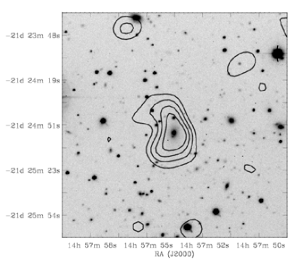
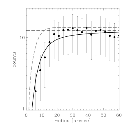
Figure 7: A specific example showing one of the major advantages of the BMW–HRI survey, i.e. its ability to detect as extended (and thus identify as groups/clusters) also sources with a very small core radius. This object, BMW145754.0-212458, has a core radius = 6″$\pm$ 2 and would not be detected as extended in a PSPC image. The optical follow–up confirmed this source as a real cD–dominated cluster at redshift at $z=0.312$. In the left panel we show a CCD $r-Gunn$ image, with HRI X–ray isophothes overlaid. The X–ray has been smoothed with a Gaussian filter ($\sigma=10\arcsec$) and the isophotes correspond to 1,1.3,1.7,2 standard deviations over the background (after smoothing). The right panel shows the measured growth curve (filled circles). The black solid line gives the integral best-fitting PSF-convolved $\beta$-model, while the grey dashed line shows the instrumental PSF at the given off-axis angle. The horizontal dashed line defines the total flux of the source, as identified by the growth curve plateau.

4 Monte-Carlo Simulations

To quantify the limitations and assess possible systematic biases in the detection procedure, we performed extensive Monte Carlo simulations under realistic conditions. First, we embedded simulated clusters and point sources within realistic backgrounds and ran the detection pipeline, in order to evaluate the completeness and the characterization uncertainties of the catalogue. Second, we ran the detection procedure on simulated fields containing pure background, thus estimating the contamination of the catalogue due to spurious detections of background statistical fluctuations. In this section we describe the simulation results in some detail.

4.1 The simulated data

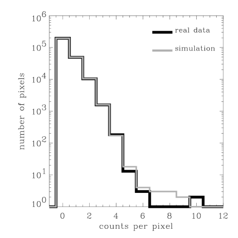
Figure 8: Comparison of the global pixel statistics of a real (black line) and a simulated image (Grey line), for a typical exposure time of 20,000 sec. X–ray photons have been binned in pixels of 5″  size. The histograms show how the background statistical properties of the simulated image accurately match those of the real one. The simulated background is built as a Poissonian realization of the background map, and the differences that can be noticed for pixels with more than five counts are due to the effect of the simulated (extended) sources, which are overabundant in the simulated image.

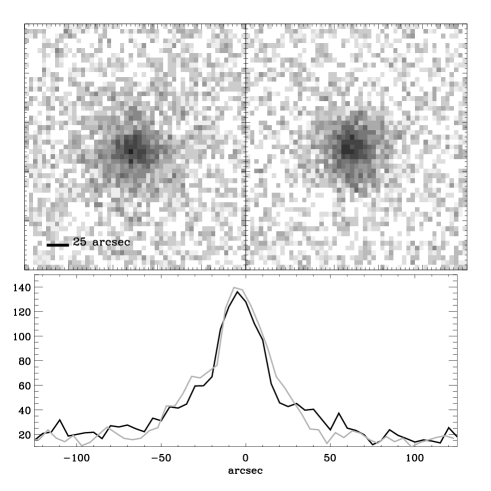
Figure 9: Top panel: visual comparison of the HRI image of BMW000141.3-154042 (left), the cluster detected with the largest number of net counts in the BMW–HRI survey, with a simulated X–ray source with the same counts and core radius. The bottom panel plots the average of the central 10 columns of the two images, with the real cluster described by the black line.

Our simulated sample consists of 12 sets of HRI fields, each set characterized by a different exposure time evenly sampling (on a logarithmic scale, see the top-right panel of Fig. 10) the range of the 914 observations which form the survey. Specific predictions for the whole set of actual exposure times are then obtained by interpolating through these 12 templates.

For each template field we used the background maps built for the BMW general catalog as described in detail in Sect. 3.3 of C99. The procedure essentially uses the ESAS software (Snowden 1994), which produces a vignetted sky background map and a background detector map. The total background map is then obtained by summing the detector and sky maps. Finally, for each simulated field a Poissonian realization of such a background is built. Fig. 8 provides an example of how the simulated background pixel statistics reproduces the observed one in a corresponding HRI image.

Point–like sources are simulated as pure PSF images with different normalizations, constructed by means of a ray–tracing technique (see C99), and their flux distribution is generated so as to reproduce the observed X–ray number counts in the [0.5-2] keV band (Moretti et al. 2003). In this way, we build a fully realistic X–ray sky, both in terms of background and surface density of point–like sources, in which to embed the simulated clusters. To construct these, we distribute counts according to a $\beta$-model surface brightness profile (Eq. 2), with values of $r_{c}$ randomly distributed in the range 5″-50″, convolved with the PSF at the specific off-axis angle where the cluster is positioned. Fig. 9 shows a visual comparison of a true cluster in the survey and a simulated one with the same core radius and integral flux. In each simulated image, we add three such extended sources, with fluxes randomly chosen in the range $10^{-14}-10^{-11}$ erg sec^-1 cm^-2. All sources (both extended and point–like) are located at random positions over the whole ($\theta=[3\arcmin-15\arcmin]$) field of view. Overall, in a typical 20 ksec image this results in a mean number of 15 sources with more than 10 counts. The rather high number of simulated clusters allows us to reach a statistically significant number of tests in a reasonable number of simulations, still avoiding detection biases due to source confusion problems. To accumulate a statistically solid test sample, the procedure is repeated 1000 times for each of the 12 template exposure times.

4.2 The catalogue completeness

As discussed in the introduction, one of the advantages of X–ray surveys of clusters is the possibility to properly quantify their selection function $S_{F}$, i.e. the probability that a source with a given set of properties (e.g. flux, extension) is detected in the survey. The selection function $S_{F}$ fully characterizes the sample completeness and is the key ingredient for estimating its sky–coverage.

In the ideal case of a uniform observation, given a value $n_{\sigma}$ for the detection threshold in S/N ratio, the corresponding minimum detectable count rate (or flux limit) can be expressed by the following formula (see e.g. ROSAT Observer Guide 1992):

$$I_{min}=\frac{n_{\sigma}b^{1/2}d_{cell}}{f_{cell}}\frac{1}{\sqrt{t_{exp}}}+\frac{C_{min}}{t_{exp}}\,\,\,\,\,.$$ (3)

Here $d_{cell}$ is the linear dimension of the detection cell , $f_{cell}$ is the fraction of signal contained in the cell, $b$ is the background count–rate and $C_{min}$ is the minimum number of source counts needed for detection when the background is negligible. However, in the low S/N regime where the source flux is comparable to the background noise, the concept of flux limit becomes somehow arbitrary: sources with fluxes lower than the theoretical sensitivity limit can be detected with non–null probability. This is due to the fact that faint sources can be detected if they sit on a positive background fluctuation, while they are missed in the opposite case. For this reason, the concept of a sharp flux limit needs to be generalized with a statistical approach, in which the selection function describes the probability for a source with given properties to be detected. Given the characteristics of X–ray telescopes and specifically of the HRI data, this probability depends in general on: i) the exposure time of the observation ; ii) the source position within the field of view: moving from the center to the edges of the images, the X–ray mirror effective area decreases and the spatial resolution worsens; iii) the source extension.

Assuming that extended sources can be sufficiently well described by the same $\beta$-model profile with different core radii, the whole cluster survey can be characterized by a selection function $S_{F}=S_{F}(f,\theta,t_{exp},r_{c})$, where $f$ is the flux, $\theta$ is the off-axis angle, $r_{c}$ is the apparent extension of the source and $t_{exp}$ the exposure time of the observation. Again, the only safe way to estimate the value of $S_{F}$ within this multi-parameter space is by means of Monte Carlo simulations.

To this end, we first grouped the input simulated sources into a grid defined by 3 different angular extension ranges, $r_{c}=[5\arcsec-20\arcsec]$, $r_{c}=[20\arcsec-35\arcsec]$, $r_{c}=[35\arcsec-50\arcsec]$, together with 20 logarithmic bins in count rate. We then considered in each of the 12 simulated sets of images, 3 different radial areas, defined by the annuli between $[3\arcmin-9\arcmin]$, $[9\arcmin-12\arcmin]$, and $[12\arcmin-15\arcmin]$ off-axis angles. At this point, we could compute the actual values of the selection function $S_{F}$ by measuring the ratio of the number of detected to the number of input simulated sources within each bin of the 4-dimensional hyper-space defined by exposure time $t_{exp}$, flux $f$, core radius $r_{c}$ and off-axis angle $\theta$. The four panels in Fig. 10 summarize the results of this procedure. The top-left panel considers a simulated field with $t_{exp}=40$ ksec and the annulus between 9′ and 12′. The points and curves show how the “projected” $S_{F}$ for different source extensions and as a function of flux is well fitted by a Fermi-Dirac function:

$$S_{F}(f,\theta,r_{c})=\frac{1}{e^{\frac{f_{50}-f}{c}}+1}$$ (4)

where $f_{50}$ and $c$ are the two free parameters of the functional form. The parameter $f_{50}$ corresponds to the flux where $S_{F}$ equals 0.5, or in other words, the detection probability equals $50\%$, while $c$ simply describes how sharp the cut-off in the selection function is.

Considering different exposure times and off-axis angles, one gets analogous plots, with different values of the pair $(f_{50},c)$. By constructing a 3-dimensional grid of the best fit $(f_{50},c)$ values over (a) 12 different exposure times, (b) 3 off–axis angles and (c) 4 core radii, we then obtain the general expression of the selection function $S_{F}$ over the whole parameter space (see panels in Fig. 10). In this way, for a source with a given core radius within the range 5″-50″, we have the detection probability for an arbitrary exposure time observation (ranging from 1 ksec to 200 ksec ), at an arbitrary position within the field of view (3′$<\leavevmode\nobreak\ \theta<$ 15′) and for an arbitrary flux (ranging from $10^{-15}$ to $10^{-11}$ erg sec^-1 cm^-2). For the few clusters with core radius larger than 50″, $S_{F}$ is safely obtained by linear extrapolation, according to the bottom-right panel of Fig. 10.

Figure 10: Dependence of the selection function $S_{F}$ on the relevant observational and source parameters, as obtained from the Monte Carlo simulations. $S_{F}$ is defined as the ratio between the number of detected over the number of simulated input sources, as explained in the text. In the top-left panel we plot the results for the annulus between off-axis angle $9\arcmin<\theta<12\arcmin$, $t_{exp}=40$ ksec and 4 different SB profiles. The points are very well fitted by a Fermi-Dirac function with different values of the two free parameters (Eq. 4). In the top-right panel for all 12 sets of simulated fields, we plot the values of $f_{50}$ (in counts sec^-1) for the region $9\arcmin<\theta<12\arcmin$ as a function of exposure time. In the bottom-left panel we plot $f_{50}$ as a function of the off-axis angle for a 5 ksec exposure and for four different source extensions. In the bottom-right panel we plot $f_{50}$ as a function of source core radii, for a 30 ksec observation in the annulus between 3′ and 10′. $f_{50}$ turns out to depend linearly also on the value of $r_{c}$. In all four plots the dashed lines reproduce the multidimensional fit as explained in the text.

4.3 The catalogue contamination

By construction, the detection threshold in the overall BMW HRI source catalogue is set by fixing the expected number of spurious sources: the higher the number of allowed spurious sources, the lower the threshold. This number is set to 1 in ten fields for each scale of the wavelet transform, which corresponds to 0.4 expected spurious sources in each frame. This, however, should be taken as a theoretical estimate because it assumes a perfectly flat background so as to provide a general instrument-independent reference (L99). Here, we derive a more accurate estimate of the number of spurious detections by properly simulating a realistic background. Moreover, due to the empirical definition of extended sources, we cannot analytically predict the number of spurious sources that will be detected as extended and need to resort again to a Monte Carlo test. To this end, we build pure background images for the usual set of 12 templates with different exposure times (and different background values) ranging from 1 ksec to 200 ksec (see Sect. 4). This time, we do not add any simulated source. For each of the 12 template images, we generate 200 different realizations of the background map, assuming a pure Poissonian noise. Then we run the BMW detection pipeline: clearly, all detected sources will be spurious, resulting from background fluctuations above the detection threshold.

Within the 2400 simulated blank frames, we detect 844 spurious sources (both point–like and extended), to be compared with the expected value of $0.4\times 2400=960$. The close agreement between these two figures represents an encouraging a posteriori confirmation that the total number of spurious detections is well under control in the whole selection procedure. Among these, 108 sources meet the requirements of our cluster survey (extension and significance), providing us with an estimate of 0.045$\pm 0.003$ spurious $p_{s}>4\,\sigma$ detections in each frame of the survey. Note that this value does not depend on the specific exposure time of the field, as in each field the detection threshold is pushed down only to the appropriate level so as to keep the total number of spurious detections constant. Given the 914 fields composing our survey, we thus expect 38$\pm 3$ spurious sources to contaminate the sample of 154 cluster candidates (25$\%$). Note that the expected number of spurious detections is proportional to the number of the analyzed fields, not related to the number of sources in the catalog. This means that, for example, if one concentrated only on a subset of high-exposure fields, the number of spurious sources would go down faster than the number of true clusters. However, the explored area and volume would also be reduced accordingly, thus affecting the ability to find luminous, rare clusters, which is one of our goals.

There is a second source of contamination that needs to be considered, which is due to point-like sources mistaken as extended. This fraction is readily estimated from our first set of simulations, where we realistically simulated the observed sky in terms of surface density distribution of point–like sources. The net result is that in the sample of 154 $p_{s}>4\,\sigma$ cluster candidates, we expect 4$\pm 2$ sources to be false classifications of a point–like source, which makes up for a total contamination of $42\pm 4$, i.e. 27$\%$.

As shown by Fig. 11, the number of total expected spurious detections (background fluctuations plus wrongly classified point-like sources), decreases significantly at higher detection significance: it is more than $40\%$ at $3\,\sigma$, $27\%$ at $4\,\sigma$ and negligible beyond $5\,\sigma$. The chosen significance threshold at $4\,\sigma$ for our main cluster catalogue is based on this plot, representing a good compromise between the total number of sources and the expected contamination.

Figure 11: The expected number of spurious detections in the BMW–HRI cluster catalogue as a function of the source significance, expressed in units of standard deviations $\sigma$ (see text for details). The curve includes the contamination produced both by background fluctuations detected as true (extended) sources and by real point sources mistaken as extended by the algorithm. On the basis of this curve, the BMW–HRI $p_{s}>4$ master sample is expected to have a 27% contamination, while selecting at $p_{s}>5$ one obtains a sample with virtually null contamination.

5 Sky Coverage and Number Counts

5.1 The BMW–HRI Cluster Survey Sky–coverage

Figure 12: The solid angle covered by the BMW–HRI survey (sky–coverage) as a function of flux and source extension, obtained by integrating the survey selection function over the observed fields.

The sky–coverage $\Omega$ (SC hereafter), measures the actual surveyed area of the survey as a function of X–ray flux and of the other parameters characterizing each source: it is a necessary ingredient for any statistical computation involving the mean surface density of clusters in the catalogue, like e.g. the log N –log S or the luminosity function.

By definition, it is closely related to the survey selection function, which, as we have seen, depends also on the off-axis angle $\theta$ and the source size $r_{c}$ (see Sect. 4.3). Let us therefore consider an infinitesimal annulus at an off-axis angle $\theta$, characterized by a solid angle $d\omega$, within the field of view of a generic observation $i$. The area of this elementary surface will contribute differently to the total sky coverage, depending on the flux limit one chooses and on the source size: for example, depending on the exposure time of the observation, it will provide its full area at a given bright flux, while it will be “invisible” at fainter fluxes. Or, equivalently, it will be effective for finding very small sources, and become ineffective for very large, blurred sources. All these effects are already taken into account by the selection function $S_{F}$ that we have carefully estimated through our Monte Carlo simulations. In fact, by definition, the actual contribution of this annulus to the total sky coverage will be

$$d\Omega_{i}=d\Omega_{i}(f,\theta,r_{c})=S_{F_{i}}(f,\theta,r_{c})d\omega\,\,\,\,\,,$$ (5)

and the total SC yielded by that given field $i$ for a source with flux $f$ and size $r_{c}$ will then be simply the sum over the annuli, i.e.

$$\Omega_{i}(f,r_{c})=\int_{\theta_{min}}^{\theta_{max}}S_{F_{i}}(f,\theta,r_{c})d\omega(\theta)\,\,\,\,\,,$$ (6)

where in our case $\theta_{min}=3\arcmin$ and $\theta_{max}=15\arcmin$. Finally, the overall SC of the survey, $\Omega_{BMW}(f,r_{c})$ will be given by the sum of the contributions by each single observation:

$$\Omega_{BMW}(f,r_{c})=\sum_{i}\Omega_{i}=\sum_{i}\int_{\theta_{min}}^{\theta_{max}}S_{F}(f,\theta,r_{c})d\omega(\theta)\,\,\,\,\,,$$ (7)

which shows explicitly the dependence of the total sky coverage on the source extension $r_{c}$ (Fig.12). Thus, given an observed source characterized by an $(f,r_{c})$ pair, it will always be possible to give a value for the total solid angle over which that source could have been found in the survey.

Given the various dependences we have discussed, a comparison of the sky coverages as a function of X–ray flux among different surveys can only be done in an approximate way, i.e. considering a “typical” sky coverage for each specific survey (e.g. Rosati et al. 2002). To perform such a comparison, given that the source extensions correlate with their fluxes (Fig. 6), we tried and obtain a sufficiently realistic one-dimensional $\Omega(f)$ by computing the mean $r_{c}$ values within 5 bins in flux, and then constructing a “composite” 1D sky coverage which in each flux range reflects the typical size of sources with that mean flux. The result is shown in Fig. 13, compared to the sky coverages of three other representative surveys from the literature. This plots shows that the BMW–HRI survey is competitive with existing PSPC surveys both at bright and faint fluxes. In particular, it provides an interesting solid angle coverage below 6$\times$10^-13 erg sec^-1 cm^-2, which results in the potential ability to detect a few clusters beyond $z\sim 0.9-1$. In fact, among the few BMW–HRI clusters with confirmed spectroscopic redshift, we already have two objects at $z=0.89$ and $z=0.92$. We remark that these values are specific for the low-contamination $p_{s}>4\,\sigma$ sample. In Sect. 5.3 we shall use this 1D sky coverage to compute the expected redshift distribution of BMW–HRI clusters.

Figure 13: Comparison of the BMW–HRI size-weighted sky coverage to those of the EMSS (Gioia et al. 1990), 160 Square Degrees (Vikhlinin et al. 1998a) and RDCS (Rosati et al. 1998). Since the sky coverage is a function of both flux and source extension, the BMW–HRI curve has been computed combining the sky coverages pertaining to different source extensions, according to the observed distribution of angular sizes in the $p_{s}>4$ sample.

5.2 Accounting for overlapping fields

As anticipated in Sect. 2.2, $7\%$ of the survey area was observed more than once. Therefore, when summing the areas contributed by each field in the sky coverage calculation we need to account for this repeated area so as to include it only once. To this end, let us consider a given source with flux $\bar{f}$, which has been observed $N$ times with different exposure times and therefore with different values of the selection function. In other words, the probability $P_{i}$ of detecting this source is different in each exposure $i$, coinciding with the value $S_{F_{i}}$of the $i$-th selection function at flux $\bar{f}$. Accordingly, the global selection function for that specific source $S_{F}(\bar{f},r_{c})$ in the N observations will correspond to the probability of detecting the source within at least one of the $N$ observations. If we consider the probability $Q$ of not detecting it in any of the observations, this is nothing else than the product of the probabilities of not detecting it in each image

$$Q=(1-P_{1})\times(1-P_{2})\times...(1-P_{N})=\prod_{i}(1-S_{F_{i}})\,\,\,\,\,.$$ (8)

At this point, the selection function pertaining to that source, $S_{F}(f,r_{c})$ will be just the complement of $Q$, i.e.

$$S_{F}=1-\prod_{i}(1-S_{F_{i}})\,\,\,\,\,.$$ (9)

5.3 The expected redshift distribution

Using the computed sky coverage, we can now address one of the most interesting aspects of a deep cluster survey, i.e. the expected redshift distribution of the sample. In particular, it is of interest to ask how many clusters we expect in the cosmologically interesting range $z\sim 1$, if any, in different evolutionary scenarios.

Briefly, the differential redshift distribution is obtained in the standard way as

$${dn\over dz}={dn\over dV}{dV\over dz}={dn\over dV}{dV\over dl}{dl\over dz}\,\,\,\,,$$ (10)

where $dl/dz$ is the cosmological comoving line element, $dV/dl=d_{A}^{2}\,d\omega$, $d_{A}$ is the angular size distance and $d\omega$ is the elementary solid angle covered (e.g. Peebles 1993, pag. 331). The sky coverage enters here when we integrate over the whole observed solid angle, while $dn/dV$, i.e. the number of clusters per unit volume expected at the same $z$, is obtained by integrating the XLF from the minimum allowed luminosity (at that $z$) to infinity,

$${dn\over dV}(z)=\int_{L_{min}(z)}^{\infty}{dn\over{dL_{X}\,dV}}dL_{X}=\int_{L_{min}}^{\infty}\phi(L_{X})dL_{X}\,\,\,\,,$$ (11)

where $\phi(L_{X})$ is very well described by the usual Schechter functional form, yielding

$${dn\over dV}(z)=\int_{L_{min}}^{\infty}\phi^{\displaystyle\ast}\left({L_{X}\over L^{\displaystyle\ast}_{X}}\right)^{-\alpha}\exp{(-L_{X}/L^{\displaystyle\ast}_{X})}\,{dL_{X}\over L^{\displaystyle\ast}_{X}}\,\,\,\,.$$ (12)

We therefore used the XLF parameters for the [0.5-2] keV band measured by the REFLEX survey (Böhringer et al. 2002), re-computed for a lambda-cosmology by Mullis et al. (2004), $\phi^{\displaystyle\ast}=8.56\times 10^{-7}\,{\rm h}^{3}$ Mpc^-3, $L^{\displaystyle\ast}_{X}=1.295\,{\rm h}^{-2}$ erg sec^-1, $\alpha=-1.69$, to obtain the solid curves shown in Fig. 14, under the hypothesis of a non-evolving XLF. Rosati et al. (2000) first used a Maximum-Likelihood approach to quantify in a phenomenological way the evolution observed in the XLF measured from the RDCS. To this end, they parameterized evolution in density and luminosity through a simple power-law model, in which

$$\phi^{\displaystyle\ast}(z)=\phi^{\displaystyle\ast}_{0}\,(1+z)^{A}\,\,\,\,,$$ (13)

$$L^{\displaystyle\ast}_{X}(z)=L^{\displaystyle\ast}_{X}{{}_{0}}\,(1+z)^{B}\,\,\,\,$$ (14)

and $\phi^{\displaystyle\ast}_{0}$, $L^{\displaystyle\ast}_{X}{{}_{0}}$ are the XLF parameter values at the current epoch. From their analysis of the RDCS survey they estimated $A=-1.2$, $B=-2$, indicating a statistically significant evolution in the mean density of luminous clusters. The same model has recently been applied to the 160SD survey data by Mullis et al. (2004), where also the EMSS, NEP and RDCS constraints are added. By comparing all these available estimates, they suggests that the best fitting values for the parameters A and B are $A\sim 0$, $B\sim-2.5$. These are the values we adopted for our computations of the expected number of clusters in the BMW–HRI survey with evolution of the XLF.

The overall results, with and without evolution, are compared in Fig. 14. The first interesting point to notice concerns the total number of clusters predicted in the two scenarios. We have a prediction of a total of 89 to 132 clusters in the $p_{s}>4$ sample, depending on evolution. Our current number of candidates is 154, with a prediction of 42 being spurious due mostly to background fluctuations. This yields a number of 112 true clusters in the survey, which is right between the predictions of the two curves. This is interesting, as it could imply that less evolution of the XLF is seen in the BMW–HRI sample. However, note that the simple (A,B) evolutionary model has been applied in the original form (Borgani et al. 2001), which, taken at face value, while reproducing correctly the observed deficit of luminous clusters above $z\sim 0.6$, also under-predicts the number of intermediate-redshift systems, as can be seen from the left panel of Fig. 14, where the two curves already begin to separate at at redshifts as low as $z=0.15$, where we know that no evolution whatsoever is observed. One possibility is to change slightly the Borgani et al. functional form describing the evolution of the XLF, as done by Mullis et al. (2004), by introducing an effective non-zero reference redshift in Eq. (13) and (14) which shifts the “switch-on” of evolution to larger, more realistic redshifts.

The second interesting point to be appreciated from the figure is the significant number of high redshift systems that the BMW–HRI survey should be capable of detecting. Even with the strongest evolution of the XLF we expect 3 clusters with $z>0.8$, with the number rising quickly to $\sim 10$ if milder evolution is admitted. In fact, we already have three confirmed clusters in this range (see Sect. 6), with a handful of further confirmed candidates with photometric redshift $>0.7$. One of these is an extremely promising object showing a concentration of galaxies with $r-Ks=[5.5-6]$ around the X–ray source position, with a range of colours typical of early-type galaxies at $z\sim 1.2-1.3$ (see e.g. Stanford 1997).

Figure 14: The expected redshift distribution of the BMW–HRI cluster sample, in differential form (left), showing the number of clusters expected in bins of $\Delta z=0.1$, and in integral form (right), showing the number of clusters expected above a given redshift $z$. The dashed curves in both panels refer to an empirical evolution model for the XLF as defined by Rosati et al. (2000), using a conservative pair of parameters (A=0,B=-2.5), which best describe the overall behaviour of available PSPC surveys (Mullis et al. 2004).

5.4 The $LogN--LogS$

The cluster number counts (historically known also as the “$LogN--LogS$” distribution) are the simplest diagnostic of cosmology/evolution that can be obtained from a sample of cosmological objects, without knowing their distances. It also represents a basic test for the quality of the sample and/or the reliability of the sky coverage, being sensitive to residual biases and contaminations as a function of flux.

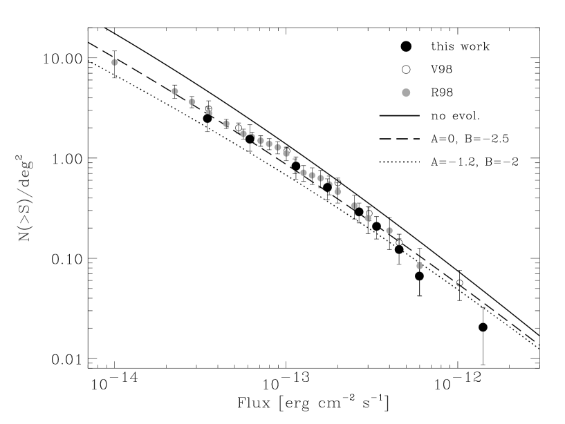
Figure 15: The classical $LogN--LogS$ plot — i.e. the mean cumulative surface density of clusters as a function of X–ray flux — from the BMW–HRI survey (filled circles), compared to the RDCS (Rosati et al. 1998) and 160SD survey (Vikhlinin et al. 1998b). The BMW–HRI points are computed from the high-significance $p_{s}>5\,\sigma$ sub-sample, for which the expected contamination is negligible. The curves give the expected counts in the same $\Lambda$-cosmology adopted in this paper, for the cases of no-evolution and evolution of the XLF. The BMW-HRI and PSPC data are all consistent with a negligible to moderate evolution of the XLF.

To compute the integral flux distribution, we weight each source by the inverse of the total area in the survey over which the source could have been detected. This is nothing else than the inverse of the sky–coverage value at the specific source flux and extension:

$$n(>S)=\sum_{f>S}\frac{1}{\Omega_{f}}\,\,\,\,\,.$$ (15)

We used this formula and the estimated sky coverage to compute the number counts using a “high-purity” sample with $p_{s}>5\,\sigma$, containing 45 candidates, for which negligible contamination is expected (Fig. 11). After estimating the appropriate sky coverage for this selection we computed the points reported in Fig.15. We chose to bin the counts so as to have an equal increase $\Delta N=5$ in the number of sources included in each bin, when moving to fainter and fainter fluxes. The error bars also include the uncertainty in the measured $r_{c}$, on which the sky coverage for each source depends. Our result is compared to similar measurements from the RDCS (Rosati et al. 1998) and 160SD (Vikhlinin et al. 1998a) surveys, and to the predictions for an unevolving and evolving XLF in the adopted $H_{o}=70$ km s^-1 Mpc^-1, $\Omega_{M}=0.3$, $\Omega_{\Lambda}=0.7$ cosmology. The XLF evolution is described using the same phenomenological $(A,B)$ model used in the previous section, here using both the original parameters by Rosati et al. (2000, dotted line) and the milder values by Mullis et al. (2004, dashed line). We also note that the no-evolution curve is slightly higher than the one shown in Rosati et al. (2002), due to the different XLF parameters used here (REFLEX vs. BCS). The main result from this plot is that the BMW-HRI and PSPC data agree very well with each other and are globally consistent with a moderate evolution of the XLF. The observed counts can be taken first of all as an a posteriori confirmation of the predicted low level of contamination of the $p_{s}>5\,\sigma$ sample, and of the self-consistency of the computed sky coverage. More substantially, the agreement with the other surveys indicates that the bulk of the (faint) cluster population is consistently detected by both PSPC- and HRI-based surveys. However, one should keep in mind also the limitations of this kind of plot. In fact, the shape and amplitude of the logN-LogS is mainly sensitive to the faint/intermediate range of the XLF (dominated by low-redshift groups and clusters), while it is rather insensitive to changes in the number of rare, high-luminosity clusters at high redshift.

6 Early follow-up results

To provide a first hint of the general optical properties of BMW-HRI clusters, we briefly summarize here some early results from the ongoing follow-up campaign. Our main cluster identification strategy is currently based on multi-band imaging in the optical $g$, $r$, $i$ bands and near-infrared $J$, $H$, $K_{s}$ bands, with at least two, typically three of these bands secured for each target. A cluster is considered as confirmed when a significant over-density of galaxies with coherent colours is detected in the area of the X–ray source. The current identification statistics, based on a total sample of 119 candidates observed so far, gives 83 confirmed, 19 rejected and 17 still uncertain clusters, in substantial agreement with the contamination level estimated in this paper. Photometric redshifts for these objects are also estimated either approximately from the mean colour of the cluster red sequence (when present), or more accurately using the photo-$z$ codes of Fernandez-Soto et al. (2001), and Bolzonella et al. (2000) when 3 or more bands are available. A few of these clusters have also been observed spectroscopically by us or have been found to be in common with other surveys. We cross-correlated our list with the latest version of the 160SD survey, with the unpublished RDCS catalogue and with the SHARC (Romer et al. 2000) and WARPS (Perlman et al. 2002) published lists. This comparison to PSPC-based surveys, performed early in the project, provided us with encouraging confirmations, indicating that the survey had the potential to efficiently peer into the high-redshift Universe. Common high-redshift clusters include, for example: $\bullet$ BMW122657.3+333253 at $z=0.888$, first discovered by Cagnoni et al. (2001) in the WGA survey and by Ebeling et al. (2001b) in the WARPS survey; $\bullet$ BMW052215.8-362452 at $z=0.53$, also found in the 160SD survey (Mullis et al. 2003); $\bullet$ two (unpublished) RDCS clusters at $z=0.64$ and $z=0.808$ (Rosati, private communication). Our current list of new high-redshift clusters includes another 7 confirmed objects reliably located at $z_{phot}>0.6$ by $r$-$i$-$Ks$ photometric redshifts. A few of these are shown in Fig. 16. These clusters will be the subject of specific future papers. X–ray/optical overlays and RGB images for more BMW–HRI clusters can be seen at http://www.merate.mi.astro.it/$\sim$guzzo/BMW/gallery.html.

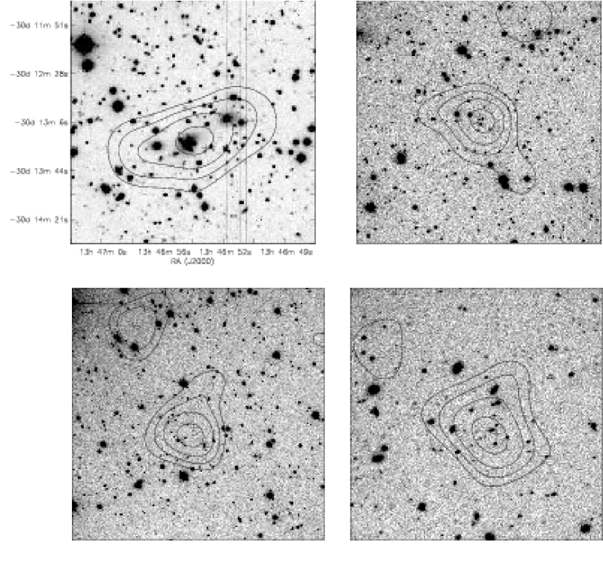
Figure 16: Optical/X–ray overlays for a selection of new BMW–HRI groups/clusters at different redshifts. From top left to bottom right: BMW134654.9-301328, $z_{spec}=0.358$; BMW212415.7-334754, $z_{spec}=0.92$; BMW122842.6-391612, $z_{phot}\simeq 0.8$; BMW112059.0+130450, $z_{spec}=0.615$. The redshift for BMW212415.7-334754, a very compact cluster, awaits further confirmation, being based on only 3 redshifts and displaying a second system at $z=0.62$. The X–ray images have been smoothed with a Gaussian filter ($\sigma=40\arcsec$) and the isophotes correspond to 0.7,1,2,3 standard deviations over the background (after smoothing). Optical images are combined $Gunn$-$r+i$ $\sim 60\min$ total exposures with EFOSC2 at the ESO 3.6 m telescope. For all but the first object the sides of the figures are 2.5′.

7 Summary and Conclusions

We have presented in detail the construction of the BMW–HRI Cluster Survey, a new sample of X–ray selected cluster candidates drawn from the so-far poorly explored ROSAT HRI archive. We have shown that by selecting sources with detection significance larger than $4\,\sigma$ and extension significance better than $\sim 3.5\,\sigma$, one can obtain a reliable sample of 154 cluster candidates with flux larger than $2\times$10^-14 erg sec^-1 cm^-2 and very interesting properties. We have performed extensive Monte Carlo simulations to recover the survey selection function with respect to the major parameters affecting the source detection. These have allowed us to reconstruct a sky coverage which is competitive with existing PSPC surveys over the whole range of fluxes, with a particularly interesting solid angle covered in the faintest bins. These results show that, contrary to expectations, the HRI data — once they have been treated as discussed in C99, i.e. eliminating the noisiest energy channels — allow us to detect low-surface-brightness objects out to high redshifts, despite their higher instrumental background. We also estimated the expected sample contamination due to background fluctuations and false classifications, which turns out to be $27\%$ for this significance threshold.

We have used a high purity sample selected at $p_{s}>5\,\sigma$, containing 45 objects expected to be virtually all true clusters, to estimate the cluster number counts in the range $3\times$10^-14 to $\sim 1\times$10^-12 erg sec^-1 cm^-2. This measurement is in very good agreement with previous estimates from the RDCS and 160SD surveys.

Possibly the most important aspect of the BMW–HRI cluster survey is that it will be the first large sample of clusters to be drawn from an instrument independent from and with higher resolution than the ROSAT PSPC, on which virtually all serendipitous cluster surveys so far have been based. This means that the BMW–HRI survey potentially includes some types of object which could have been missed in previous surveys. It is natural to expect that these are mostly small groups, which the HRI is able to detect as extended. Indeed, we have specific examples in the survey of objects with core radii as small as 6″. The observed agreement among our number counts and those from the RDCS and 160SD surveys, however, indicates that the percentage of these small-sized objects does not seem to be sufficient to represent a substantial incompleteness in PSPC surveys. A finer assessment of possible differences will be provided once the redshifts for BMW–HRI clusters are measured, both by comparison of the faint end slopes of the cluster XLF and of the number of clusters detected above $z\sim 0.8$. While the faint end of the number counts is dominated by low-redshift, low-luminosity objects, the HRI resolution should begin to make a difference when one goes to high redshifts. The work of Ettori et al. (2004), based on Chandra observations, seems to indicate that $z>0.8$ clusters have on average a more compact profile than their lower-redshift counterparts. Keeping in mind that all our simulations are based on the necessary but crude approximation of a $\beta=2/3$ profile, these findings would go in the direction of increasing the probability of detecting clusters at high redshift, favored by the HRI high spatial resolution. This would probably be too mild to show a significant effect in the integral number counts, yet might increase the number of detectable $z\sim 1$ clusters by a significant factor.

- (1) Allen, S.W., Schmidt, R.W., Fabian, A.C., 2001, MNRAS, 328, L37
- (2) Arena, S., 2002, Laurea Thesis, Università di Milano Bicocca
- (3) Blakeslee, J.P., Franx, M., Postman, M. et al., 2003, ApJ, 596, 143
- (4) Böhringer, H., Schuecker, P., Guzzo, L., et al., 2001, A&A, 369, 826
- (5) Böhringer, H., Collins, C.A., Guzzo, L., et al., 2002 ApJ, 566, 93
- (6) Böhringer, H., Schuecker, P., Guzzo, L., et al., 2004, A&A, in press
- (7) Bolzonella, M., Miralles, J.-M., Pellò, R., 2000, A&A, 363, 476
- (8) Borgani, S., Guzzo, L., 2001, Nature 409, 39
- (9) Borgani, S., Murante, G., Springel, V., et al., 2004, MNRAS, 348, 1078
- (10) Borgani, S., Rosati, P., Tozzi, P., et al., 2001, ApJ, 561, 13
- (11) Boschin, W., 2002, A&A, 396, 397
- (12) Cagnoni, I., Elvis, M., Kim, D.W., et al., 2001, ApJ, 560, 860
- (13) Campana, S., Lazzati, D., Panzera, M.R., Tagliaferri, G., 1999, ApJ, 524, 423 (C99).
- (14) Cavaliere, A., Fusco–Femiano, R., 1976, A&A, 49, 137
- (15) Collins C.A., Burke D.J., Romer A.K., 1997, ApJ, 479, 117L
- (16) David, L.P., et al., 1998, The ROSAT HRI Calibration Report, U.S. ROSAT Science Data Center (SAO)
- (17) De Grandi, S., Guzzo, L., Böhringer, H., et al., 1999, ApJ, 513, 17
- (18) Dickey, J.M., Lockman F.J., 1990, ARA&A, 28, 215
- (19) Ebeling, H., Edge, A.C., Fabian, A.C., et al., 1997, ApJ, 479, L101
- (20) Ebeling, H., Jones, L.R., Fairley, B.W., et al., 2001a, ApJ, 548, L23
- (21) Ebeling, H., Edge, A.C., Henry, J.P., et al., 2001b, ApJ, 553, 668
- (22) Ettori, S., Tozzi, P., Borgani, S., Rosati, P., 2004, A&A, 417, 13
- (23) Evrard, A.E., Metzler, C.R., Navarro, J.F., 1996, ApJ, 469, 494
- (24) Fern ndez-Soto, A., Lanzetta, K.M., Chen, H.W. Pascarelle, Sebastian M., Yahata, N., 2001, ApJS, 135, 41
- (25) Finoguenov, A., Reiprich T.H., Böhringer, H., 2001, A&A, 368, 749
- (26) Gioia, I., Maccacaro, T., Schild, R.E., et al., 1990, ApJS, 72, 567
- (27) Gioia, I.M., Henry, J.P., Mullis, C.R., Voges W., Briel U.G., 2001, ApJ, 553, L105
- (28) Gioia, I.M., Henry, J.P., Mullis, C.R., 2003, ApJS, 149, 29
- (29) Helsdon, S.F., Ponman, T.J., 2000, MNRAS, 315, 356
- (30) Gioia, I., Henry, J.P., Mullis, C.R., et al., 2003, ApJS, 149, 29
- (31) Henry, P., Gioia, I.M., Maccacaro T., et al., 1992, ApJ, 386, 408
- (32) Kaiser, N., 1986, MNRAS, 222, 323
- (33) Lazzati, D., Campana, S., Rosati., P., et al., 1999, ApJ, 524, 414 (L99)
- (34) Lidman, C., Rosati, P., Demarco, R., et al., 2004, A&A, 416, 829
- (35) Mohr, J.J., Reese, E.D., Ellingson, E., et al., 2000, ApJ, 544, 109
- (36) Moretti, A., Campana, S., Lazzati, D., Tagliaferri, G., 2003, ApJ, 588, 696
- (37) Mullis, C.R., McNamara, B.R., Quintana, H., et al., 2003, ApJ, 594, 154
- (38) Mullis, C.R., Vikhlinin, A., Henry, P., et al., 2004, ApJ, in press (astro-ph/0401605)
- (39) Nichol R.C., Romer, A.K., Holden, B.P., et al., 1999, ApJ, 521, L21
- (40) Panzera, M.R., Campana, S., Covino, S., et al., 2003, A&A, 399, 351 (P03)
- (41) Peacock, J.A., 1999, Cosmological Physics, Cambridge University Press, Cambridge.
- (42) Peebles, P.J.E., 1993, Principles of Physical Cosmology, Princeton University Press
- (43) Perlman E.S., Horner D.J., Jones L.R., 2002, ApJS, 140,265
- (44) Pierpaoli, E., Borgani, S., Scott, D., White, M., 2003, MNRAS, 342, 16
- (45) Prestwich, A., Callanan, P., Snowden, S., et al., 1996, A&AS, 189, 905
- (46) Romer, A.K., Nichol, R.C., Holden, B.P., et al., 2000, ApJS, 126, 209
- (47) Reiprich, T.H., Böhringer, H., 2002, ApJ 567, 716
- (48) Rosati, P., Della Ceca, R., Burg, R., et al., 1995, ApJ, 445, L11
- (49) Rosati, P., Della Ceca, R., Burg, R., Norman, C., Giacconi, R., 1998, ApJ, 492, L21
- (50) Rosati, P., Borgani, S., Della Ceca, R., et al., 2000, in Large-Scale Structure in the X-ray Universe, M. Plionis & I. Georgantopulos eds., Atlantisciences, Paris, p. 13
- (51) Rosati, P., Borgani, S., Norman, C., 2002, ARA&A, 40, 539
- (52) Schuecker, P., Böhringer, H., Collins, C.A., et al., 2003, A&A, 398, 867
- (53) Snowden, S. L. 1994, Cookbook for analysis procedures for ROSAT XRT/PSPC observations of extended objects and diffuse background
- (54) Stanford, S. A., Elston, R., Eisenhardt, P.R., et al., 1997, AJ, 114, 2232
- (55) Valtchanov, I., Pierre, M., Willis, J., et al., 2003, A&A, in press (astro-ph/0305192)
- (56) Vikhlinin, A., McNamara, B.R., Forman, W., et al., 1998a, ApJ, 498, L21
- (57) Vikhlinin, A., McNamara, B.R., Forman, W., et al., 1998b, ApJ, 502, 558
- (58) Voges, W., Aschenbach, B., Boller, Th., et al., 1999, A&A, 349, 389