The Parkes quarter-Jansky flat-spectrum sample

We analyze the Parkes quarter-Jansky flat-spectrum sample of QSOs in terms of space density, including the redshift distribution, the radio luminosity function, and the evidence for a redshift cutoff. With regard to the luminosity function, we note the strong evolution in space density from the present day to epochs corresponding to redshifts $\sim 1$. We draw attention to a selection effect due to spread in spectral shape that may have misled other investigators to consider the apparent similarities in shape of luminosity functions in different redshift shells as evidence for luminosity evolution. To examine the evolution at redshifts beyond $3$, we develop a model-independent method based on the $V_{\rm max}$ test using each object to predict expectation densities beyond $z=3$. With this we show that a diminution in space density at $z>3$ is present at a significance level $>4\sigma$. We identify a severe bias in such determinations from using flux-density measurements at epochs significantly later than that of the finding survey. The form of the diminution is estimated, and is shown to be very similar to that found for QSOs selected in X-ray and optical wavebands. The diminution is also compared with the current estimates of star-formation evolution, with less conclusive results. In summary we suggest that the reionization epoch is little influenced by powerful flat-spectrum QSOs, and that dust obscuration does not play a major role in our view of the QSO population selected at radio, optical or X-ray wavelengths.

1 Introduction

This is the last in a series of three papers describing the results of a program to search for high-redshift radio-loud QSOs and to study the evolution of the flat-spectrum QSO population.

Paper 1 (Jackson et al. 2002) set out the sample, discussing selection, identification and reconfirmation programmes to determine the optical counterparts to the radio sources. Paper 2 (Hook et al. 2003) presented new spectroscopic observations and redshift determinations. This paper considers the radio-loud QSO space distribution, the epoch-dependent luminosity function, the evidence for a redshift cutoff provided by the sample, and the form of this cutoff.

Paper 1 described how the identification programme for 878 flat-spectrum radio sources selected from the Parkes catalogues yielded a near-complete set of optical counterparts. Indeed for the sub-sample at declinations above $-$40^∘ with flux densities above catalogue completeness limits, only one source remains unidentified. Of the 379 QSOs in this sub-sample, 355 have measured redshifts, obtained from earlier observations and the extensive spectroscopy programme described in Paper 2. This relative completeness is ideal for studies of space density, as it becomes possible to map the entire “quasar epoch” with a single homogeneous sample, having no optical magnitude limit and free of obscuration effects. In fact a sub-sample of objects from an earlier analysis was used by Shaver et al. (1996) to study the evolution of QSO space density at high redshifts. The study showed that the space density of high-luminosity radio QSOs decreased significantly at redshifts beyond 3. Preliminary data were also used by Jackson & Wall (1999) in considering a dual-population scheme of space densities for unified models of QSOs and radio galaxies.

General features of the luminosity function and its redshift dependence have long been established for QSOs selected at optical and radio wavelengths (e.g. Longair 1966; Schmidt 1968; Fanti et al. 1973). Powerful evolution is required, similar in magnitude for selection at either waveband; the space density of the more luminous QSOs at redshifts of 1 to 2 is at least $10^{2}$ that at the present epoch. It has been hotly debated as to whether the form of this change is luminosity evolution (e.g. Boyle et al. 1988) or luminosity-dependent density evolution (e.g. Dunlop & Peacock 1990). It does not matter: physical models are not available that require either form, although it is clear that luminosity evolution results in lifetimes of non-physical length (Haehnelt & Rees 1993, and references therein). The space density of radio-selected QSOs, constituting some 10 per cent of all QSOs, generally appears to parallel that of optically-selected QSOs (e.g. Schmidt et al. 1991; Stern et al. 2000).

There are many reports of a redshift cutoff in the literature: paper after paper speaks of ‘the quasar epoch’, ‘a strongly-evolving population peaking at a redshift of about 2’, or ‘the quasar redshift cutoff’ without specific reference. For optically-selected QSOs, several classic studies demonstrated that such a cutoff does exist (Schmidt et al. 1991; Warren et al. 1994; Kennefick et al. 1995). The Sloan Digital Sky Survey (SDSS) has now found QSOs out to redshifts beyond 6, and analyses of the space density (Fan et al. 2001a, c, b) provide the strongest evidence to date of the drop in space density beyond $z=3$. X-ray surveys now appear to show that the X-ray QSO population exhibits a decline at high redshifts similar to that found for optically-selected QSOs (Hasinger 2003; Barger et al. 2003; Silverman et al. 2004). But do all these observations indicate a real diminution or – at least at optical wavelengths – could it be due to a dust screen (Heisler & Ostriker 1988; Fall & Pei 1993)? It is here that radio-selected samples such as the present one can provide a powerful check: if a significant diminution is seen in the radio luminosity function, it cannot be the result of dust obscuration. Dunlop & Peacock (1990) presented some evidence for just such a cutoff of the radio luminosity function (RLF) for flat-spectrum (QSO-dominated) populations; and an earlier analysis of a sub-sample from the present work (Shaver et al. 1996) added confirmation. More recently Vigotti et al. (2003) defined a complete sample of 13 radio QSOs at $z\sim 4$, from which they concluded that the space density of radio QSOs is a factor of $1.9\pm 0.7$ smaller than that of similar QSOs at $z\sim 2$. However, Jarvis & Rawlings (2000) questioned these radio-QSO results, focussing on the possible effects of spectral curvature.

A possible dust screen has serious implications for the interpretation of the Hubble diagram for SN Ia supernovae. Assuming no obscuration, current results from the SCP (Supernova Cosmology Project) collaboration (Knop et al. 2003) and the Hi-z team (Tonry et al. 2003) favour an $\Omega_{m}=0.3,\ \Omega_{\Lambda}=0.7$ universe. Two further related issues make delineation of the QSO epoch very important: galaxy formation, and the reionization of the Universe.

1.1 Galaxy formation

The dramatic cosmic evolution of radio galaxies and QSOs stood as a curiosity on its own for over 30 years since the birth of the idea (Ryle 1955), clouded as it was in the source-count controversy (Scheuer 1990). It is relatively recently that corresponding evolution has been delineated for the star-formation rate (Lilly et al. 1996; Madau et al. 1996) and for galaxy evolution, particularly blue galaxies (Ellis 1999). The correlation between star-formation rate and AGN space density (Wall 1998) strongly suggested a physical connection (Boyle & Terlevich 1998). Before the emergence of the Lilly-Madau plot of star-formation history, it was recognized that the model of hierarchical galaxy development in a Cold Dark Matter (CDM) Universe would result in a ‘quasar epoch’ (Haehnelt 1993; Haehnelt & Rees 1993). The issue of ‘quasar epoch’ and ‘redshift cutoff’ has therefore assumed particular importance in consideration of galaxy formation in low-density CDM universes. The very existence of any high-redshift QSOs sets constraints on the epoch of formation of the first galaxies. Haehnelt (1993) showed how the then-new COBE normalization (Smoot et al. 1992) together with the QSO luminosity function at high redshifts as measured by Boyle et al. (1991), provided substantial information on the initial fluctuation spectrum and the matter mix. He found that the $z=4$ luminosity function excluded an initial-spectrum index of $n\leq 0.75$ or a Hot Dark Matter fraction $\geq 25$ per cent. Relevant to the current view of the low-matter-density CDM Universe, he found that $\Omega_{\Lambda}\leq 0.75$. Haehnelt & Rees (1993) developed a model for the evolution of the QSO population based on the existence of $\sim$ 100 generations and linking the QSO phenomenon with the hierarchical build-up of structure in the Universe. The evolution of host objects is mirrored in the evolution of the mass of newly formed black holes; only a moderate efficiency for formation of an average black hole is necessary to model the luminosity function. The model suggested that nearly all galaxies are likely to have passed through a QSO phase. Kauffmann & Haehnelt (2000) produced a more sophisticated model by incorporating a simple scheme for the growth of supermassive black holes into the CDM semi-analytic models that chart the formation and evolution of galaxies. In addition to reproducing the observed relation between bulge luminosity and black-hole mass in nearby galaxies (Magorrian et al. 1998), the model is able to mimic the enormous increase in the QSO population from redshift 0 to 2, a feature that the Haehnelt-Rees model was able to describe only qualitatively. Their conclusion: “Our results strongly suggest that the evolution of supermassive black holes, quasars and starburst galaxies is inextricably linked to the hierarchical build-up of galaxies.”

1.2 Reionization

The paradigm of hierarchical structure growth in a CDM universe has long suggested that after the recombination epoch at $z\sim 1500$, the reionization of the Universe took place at redshifts between 6 and 20 (e.g. Gnedin & Ostriker 1997). This reionization is predicted to be patchy and gradual (Miralda-Escudé et al. 2000), although some models indicate that it should happen quite rapidly (e.g. Cen & McDonald 2002; Fan et al. 2002). Two major observational advances support the ‘patchy and gradual’ scenario. Firstly, SDSS discovery of QSOs at redshifts of 6 or more (Fan et al. 2000, 2001a; Becker et al. 2001) has given a glimpse of what may be the end of the epoch of reionization: the first complete Gunn & Peterson (1965) trough has been observed in the $z=6.29$ QSO SDSS 1030+0524 (Becker et al. 2001; Pentericci et al. 2002) and a second has been seen in $z=6.43$ QSO SDSS J1148+5251 (Fan et al. 2003). There is disagreement as to whether this marks the true end of reionization (Songaila & Cowie 2002); but the suggestion is that it may be essentially complete by $z\sim 6-7$. Secondly, the detection of polarized anisotropies with the Wilkinson Microwave Anisotropy Probe (WMAP) has resulted in a measurement of the optical depth $\tau\sim 0.17$ to Thompson scattering (Bennett et al. 2003; Kogut et al. 2003), implying a reionization redshift of $17\pm 5$. The CMB is sensitive to the onset of ionization, while Gunn-Peterson troughs are sensitive to the late stages, the cleanup of remaining HI atoms. Resolving the large uncertainties in these redshifts could yet result in a rapid reionization scenario. Nevertheless several recent papers (see e.g. Haiman & Holder 2003) address the complex and interacting suite of physical mechanisms that may be at play during an extended ‘patchy and gradual’ reionization epoch $6<z<17$.

In either a fast or a gradual scenario, identifying the source of this reionization as well as epoch is of vital importance for such interconnected reasons as:

• The role of reionization in allowing protogalactic objects to cool into stars,

• The small-scale temperature fluctuations in the CMB and how these are influenced by patchiness in the reionization, and

• The epoch of the first generation of stars, or galaxies, or collapsed black-hole systems.

It is most likely that the reionization is via photoionization by UV radiation from stars or QSOs, rather than collisional ionization in e.g. blast waves from the explosive deaths of Population III stars (Madau 2000). It may be possible to detect this reionization epoch directly as a step in the background radiation at radio frequencies between 70 and 240 MHz (redshifted 21-cm HI) or in the infrared, 0.7 to 2.6 $\mu$m, from H recombination (Shaver et al. 1999). It may be possible with results from the Planck mission to identify features in the CMB that identify what the predominant mechanisms are; and it may be possible to detect the UV sources responsible for the ionizing flux at $z\sim 10-20$ with the James Webb Space Telescope (Haiman & Holder 2003).

QSOs have long been prime candidates for this reionization. However the apparent decline in space density (from the evidence summarized above and by Madau et al. 1999), is inconsistent with this interpretation. Madau (2000) showed that in the face of this apparent diminution, UV luminosity functions of Lyman-break galaxies (LBG) provide 4 times the estimated QSO contribution at $z=3$. It is now commonly accepted that such objects (or their progenitor components) take on the mantle. The formation of short-lived massive stars in such galaxies provides the UV photons (Haehnelt et al. 2001), although QSOs may supply a significant fraction of the UV background at lower redshifts.

Because the cooling time is long, the low-density IGM retains some memory of when and how it was ionized. Several investigators have found a peak in temperature of the IGM at $z\sim 3$ (Schaye et al. 2000; Theuns et al. 2002) close to the peak of the ‘quasar epoch’. Moreover, observations of several QSOs at the wavelength of HeII Ly$\alpha$ near $z=3$ suggest delayed reionization of He I, with the process not yet complete by $z=3$ (Kriss et al. 2001). The implication is that the QSO ionizing photons coincident with the peak in activity both reionize HeI and dump entropy into the IGM to raise its temperature.

In all of these aspects, it is clear that conclusions on ionizing flux from QSOs are dependent on poorly determined high-power regions of luminosity functions, on apparent cutoffs observed primarily in optically-selected samples, and then only for the most luminous QSOs.

It is a primary purpose of this paper to determine the radio luminosity function using the near-complete data of the present sample, and to examine the evidence for a redshift cutoff. Before this, we discuss the populations involved in the flat-spectrum sample by examining the $N(z)$ relation (§ 2). Subsequent to the RLF determination in § 3, we consider the issue of a redshift cutoff (§ 4), and the form of this cutoff. In § 5 we construct an overall picture of epoch dependence of space density for radio-loud QSOs. We compare this with the parallel results for QSOs selected at optical and X-ray wavelengths, and with the behaviour of star-formation rate with epoch. The final section (§ 6) summarizes results from this paper and our preceding two papers.

2 The redshift distribution

For a sample of objects complete to some flux-density limit, the redshift distribution, $N(z)$, gives preliminary information on the epoch of the objects, and allows the most direct comparison with other samples. The redshift distribution gives direct information on neither the luminosity function nor its epoch dependence; however it provides essential data for use with other data such as source counts to enable the construction of epoch-dependent luminosity functions. There have been many versions of this. Most are a variant on either the $V_{\rm max}$ method (Schmidt 1968) or the technique of defining the luminosity distribution (Wall et al. 1980; Wall 1983), obtained when a complete $N(z)$ is available at one flux-density level at least.

Such modelling processes now make use of statistical techniques to incorporate data sets of varying completeness at many frequencies and flux-density levels. The sample described here represents only one such data set, more complete than most. Dunlop & Peacock (1990) carried out the most extensive such modelling. They took as a starting point two populations, ‘flat-spectrum’ and ‘steep-spectrum’ radio sources, now broadly considered in the light of unified models as beamed radio sources (radio-loud QSOs and BL Lac objects) and their unbeamed progenitors, or hosts (FRI and FRII radio galaxies). All these objects are deemed to be powered by accretion-disk / rotating black-hole systems from which a pair of opposing relativistic jets feed double radio lobes. The single axis is collimated during the feeding process by rotation of the black-hole system. The beamed objects, QSOs and BL Lacs, beamed because of relativistic ejections of components along axes aligned with the line-of-sight, have radio structures dominated by relativistically-boosted core emission. This core emission shows the effects of synchrotron self-absorption and therefore has a flat or inverted radio spectrum. The radio emission from powerful radio AGN whose axes are not aligned with the line-of-sight is dominated by their steep-spectrum lobe emission, on the large scales of 10’s of Kpc up to 100’s of Mpc. The dichotomy between beamed and unbeamed objects as evidenced by their integrated radio spectra is shown in Fig. 1.

The widely-used Dunlop-Peacock models of the luminosity functions may be simply tested against the present data by means of the $N(z)$ distributions that they predict.

Figure 1: The spectral index distribution for the compilation of sources from Parkes surveys known as PKSCat90. The sub-sample selected has $S_{\rm 2.7\,GHz}\geq 0.25$ Jy, in regions surveyed to a limiting flux density of 0.25 Jy or less. The hatched area shows the sources identified as QSOs or BL Lac objects. These beamed objects dominate the ‘flat-spectrum’ region of the diagram.

We constructed a redshift distribution from the sample of Paper 1 as follows. We selected all sources with $S_{\rm 2.7\,GHz}\geq 0.25$ Jy in regions for which the 2.7-GHz flux-density limit was 0.25 Jy or less, and at declinations $2.5\hbox{${}^{\circ}$}\geq\delta\geq-40\hbox{${}^{\circ}$}$. We refer to this as Sample 1 and the total area it covers (Fig. 1 of Paper 1) is 2.676 sr. The source composition, identification and redshift data for this sample are shown in Table 1. Choice of the declination limit comes from both identification and radio-spectral completeness; see §3.

Table 1: Sample 1: an all-source sample selected from the source list of Paper 1 in order to estimate the redshift distribution: $S_{\rm 2.7\,GHz}\geq 0.25$ Jy, $S_{\rm lim}\leq 0.25$ Jy, $2.5\hbox{${}^{\circ}$}\geq\delta\geq-40\hbox{${}^{\circ}$}$.

Ident	No Redshift	Redshift	Total
QSO	20	308	328
BL	34	9	43
G	57	27	84
Obsc	2	0	2
e	1	0	1
Totals	114	344	458

The entries in the identification column, Table 1, refer to (QSO)s, (BL) Lac objects, (G)alaxies, (Obsc)ured fields, and (e) not identified for reasons discussed in Paper 1. As reasonable approximations, the 20 QSOs without measured redshifts were assumed to have the same redshift distribution as those with redshifts; likewise the unmeasured redshifts of the 34 BL Lac objects were assumed to have the same distribution as those measured. Such an approximation is inappropriate for the galaxies, however. A crude Hubble diagram was plotted for the 27 galaxies with redshifts and a simple polynomial was fitted to make rough estimates of the redshifts for the remaining 57 galaxies based on their $B$ magnitudes. Finally the 3 Obsc and e sources were assumed to have the same redshift distribution as the total sample; the $N(z)$ obtained by adding the QSO, BL Lac and galaxy redshifts was simply scaled by $(344+111+3)/(344+111)$ to obtain the final $N(z)$ of Fig. 2.

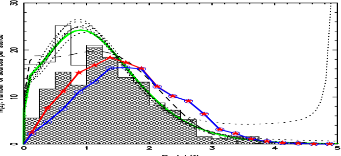
Figure 2: The redshift distribution (histogram) for the sources of Sample 1 (Table 1). The hatched area shows the redshift distribution for beamed objects alone, the QSOs + BL Lac objects, while the clear region represents the galaxies. The 6 dotted lines show the appropriately-scaled distributions predicted by the flat-spectrum ($\alpha\geq-0.5$) components of the Dunlop-Peacock (1990) luminosity-function models, with the dashed line distinguishing their pure-luminosity-evolution model. The solid line represents the average of 6 of the models, omitting the model showing the very steep rise to $z=5$. The symbol + line systems show the predictions from the dual-population models of Jackson & Wall (1999), red representing all beamed objects (QSOs + BL Lacs), blue for QSOs only.

Dunlop & Peacock derived luminosity functions for their two-population model, flat-spectrum and steep-spectrum radio sources, representing the luminosity functions as polynomials over the surface ($\rho,P_{\rm radio},z$), and obtaining coefficients by best-fitting to multi-frequency survey data including source counts and redshifts. Different models resulted from different starting points and factorizations of the epoch-dependent luminosity function. Their division between flat-spectrum and steep-spectrum sub-populations took spectral index $\alpha=-0.5$ as the dividing criterion. The predictions of redshift distributions from the flat-spectrum portions of Dunlop-Peacock luminosity functions are shown in Fig. 2. In order to scale these to our spectral-selection criterion, we used the spectral-index histogram of Fig. 1; the ratio of objects with $\alpha\geq-0.4$ (our selection criterion, Paper 1) to those with $\alpha\geq-0.5$ is 1060/1275 = 0.831.

In view of uncertainties in spectral index and of equating the flat-spectrum population of Dunlop & Peacock with compact radio sources, the overall agreement is good. The form of the decline in $N(z)$ to higher redshifts is impressively described by the Dunlop-Peacock models. Two models stand out in Fig. 2. One model with a space-density cutoff at $z=5$ predicts a redshift distribution greatly at variance with observations, showing a dominant spike in the distribution at redshifts just below this cutoff. It has been left out of the averaging process. The pure-luminosity-evolution model, shown as the dashed line, is distinct in having a quicker rise and flatter maximum than the others. These two features provide a better representation of the data in the range $0<z<1.5$ than do the other models.

The good fit of the Dunlop-Peacock models to the total $N(z)$ distribution for flat-spectrum objects does not imply a good description of the $N(z)$ for beamed objects (hatched area, Fig. 2) alone. The Dunlop-Peacock models clearly rely on the presence of low-luminosity flat-spectrum galaxies for the quality of overall fit; the ‘flat-spectrum’ models describe the beamed objects alone rather poorly.

Models considering populations in terms of beamed and host object were developed by Jackson and Wall (Wall & Jackson 1997; Jackson & Wall 1999). The $N(z)$ predictions from these models are shown in Fig. 2. Agreement is reasonable; normalization is correct, and the forms of the curves are similar. This agreement is expected on the basis of the fit of the model to the 5-GHz source count and the incorporation of a redshift cutoff in the model evolution. The models over-predict objects at $z>2$, due primarily to a lack of constraint on the evolution of low-luminosity sources.

3 The Radio Luminosity Function (RLF)

Completeness of identifications enables the radio luminosity function to be constructed in a straightforward way, using the $1/V_{obs}$ approach (Schmidt 1968; Felten 1976; Avni & Bahcall 1980). The contribution of each object to space density is calculated as the reciprocal of the observable volume, the volume defined by the redshift range(s) in which the object can be seen. Because the sample is optically complete, only radio data (apart from the redshifts) are relevant in defining this range.

An appropriate sub-sample for this calculation is that referred to as Sample 2 in Table 2. Selected from the catalogue of Paper 1, it includes all the QSO identifications with flux densities above survey limits and within the declination range +2.5^∘ to $-$40^∘. Defining $V_{obs}$ requires knowledge of the radio spectrum both above and below the survey frequency. Above 2.7 GHz, there are the 5.0-GHz data of the Parkes catalogues for all sources in the 2.7-GHz surveys, flux densities at 8.4 GHz for many of these sources (Wright et al. 1990), and about 40 8.87-GHz flux densities for some of the brighter sources (Shimmins & Wall 1973). Below 2.7 GHz, flux densities exist for most members of Sample 2 at 365 MHz from the Texas survey (Douglas et al. 1996), and at 1.4 GHz from the NRAO VLA sky survey (Condon et al. 1998). The Texas survey covers the sky at declinations down to $-$35.5^∘ and the NVSS down to $-$40^∘. As a compromise between sample size and spectral completeness, the sub-sample chosen for definition of the RLF, Sample 2 of Table 2, was therefore taken to have a southern declination limit of $-$40^∘. Most of the area surveyed at 2.7 GHz in this range has a completeness limit of $S_{\rm 2.7\,GHz}=0.25$ Jy, but some regions have limits of 0.10, 0.20 and 0.60 Jy; see Fig. 1 of Paper 1.

Table 2: QSO samples for RLF and redshift-cutoff analyses.

Sub-sample	Sample 2†		Sample 3‡
with measured z UKST ID	342		242
with measured z CCD ID	13		10
total QSOs with measured z		355		252
no measured z UKST ID	17		11
no measured z CCD ID	6		4
total QSOs with no measured z		23		15
no ID (no measured z)	1	1	1	1
Totals QSOs + non-ID	379	379	268	268

${}^{\dagger}S_{\rm 2.7\,GHz}\geq S_{\rm lim}$, $+2.5\hbox{${}^{\circ}$}>\delta>-40\hbox{${}^{\circ}$}$, area 3.569 sr.
${}^{\ddagger}S_{\rm lim}=0.25$, $S_{\rm 2.7\,GHz}\geq S_{\rm lim}$, area 2.278 sr.

The steps to defining $V_{\rm obs}$ consist of (1) determining $P_{2.7\rm\leavevmode\nobreak\ GHz}$, the luminosity of the radio source at 2.7 GHz (rest frame), and (2) ‘moving’ the source with its spectrum defined by the measured flux densities, from $0<z<\infty$ to determine in which redshift range(s) it is observable. It is observable at a given redshift if (a) its flux density exceeds the survey limit $S_{2.7}=0.25$ Jy and (b) its redshifted spectrum over the observer’s range 2.7 to 5.0 GHz has a spectral index $\geq-0.4$. We interpolated between measured spectral points in the log S_ν - log $\nu$ plane. Despite the relatively sparse sampling in this plane, combined luminosity and spectral effects of ‘moving’ the source are complex, sometimes resulting in a source having two regions of observable volume defined by four redshifts. (These effects are discussed further in the following section.) In calculating the RLF, the contribution of each source is then

$$\sum_{i}1/(V^{i}_{\rm max}-V^{i}_{\rm min})$$

where $i$ is usually unity but is sometimes two. Throughout the analyses we have used the geometry $H_{0}=70$ km s^-1 Mpc^-1, $\Omega_{\rm tot}=1.0$, $\Omega_{\rm m}=0.3$, $\Omega_{\Lambda}=0.7$.

Table 3: The radio luminosity function $\rho$, in units of log(Mpc^-3) per $\Delta z=0.5$ per $\Delta($log$P)=0.4$, as derived from Sample 2, Table 2. $N$ is the number observed per bin and $\overline{z}$ the mean redshift of the sources in the bin.

Power	$0<z<0.5$			$0.5<z<1.0$			$1.0<z<2.0$			$2.0<z<3.0$			$3.0<z<5.0$
log(P/ WHz-1sr${}^{-1})$	log$\rho$	$N$	$\bar{z}$	log$\rho$	$N$	$\bar{z}$	log$\rho$	$N$	$\bar{z}$	log$\rho$	$N$	$\bar{z}$	log$\rho$	$N$	$\bar{z}$
24.8	$-$9.02	4	0.33	$-$10.22	1	0.58	—	0	—	—	0	—	—	0	—
25.2	$-$8.60	15	0.36	$-$9.13	6	0.62	—	0	—	—	0	—	—	0	—
25.6	$-$9.54	2	0.32	$-$8.91	29	0.73	$-$10.40	5	1.11	$-$11.43	1	2.12	—	0	—
26.0	$-$10.27	1	0.36	$-$9.26	19	0.77	$-$9.57	45	1.32	—	0	—	—	0	—
26.4	$-$11.11	1	0.16	$-$9.85	15	0.78	$-$9.33	91	1.47	$-$10.34	19	2.24	$-$12.13	1	3.45
26.8	—	0	—	$-$10.35	5	0.77	$-$10.05	29	1.69	$-$10.05	34	2.48	$-$11.02	12	3.47
27.2	—	0	—	—	0	—	$-$11.00	6	1.50	$-$10.98	8	2.33	$-$11.82	2	3.45
27.6	—	0	—	—	0	—	—	0	—	$-$12.19	1	2.56	$-$12.32	1	3.57

Following these precepts, the radio luminosity functions calculated for rest-frame powers at 2.7 GHz for 5 redshift ranges are given in Table 3.

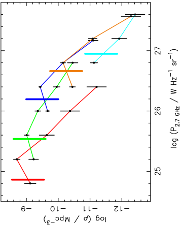
Figure 3: The radio luminosity function ($H_{0}=70$ km s^-1 Mpc^-1, $\Omega_{\rm tot}=1.0,\ \Omega_{\rm m}=0.3,\ \Omega_{\Lambda}=0.7$) for the QSOs of the Parkes 0.25-Jy flat-spectrum sample. The RLF was computed in redshift ranges $0-0.5$ (red), $0.5-1.0$ (green), $1.0-2.0$ (blue), $2.0-3.0$ (orange) and $3.0-5.0$ (light blue). Vertical bars show the limits of completeness in power for each redshift range, as described in the text. Error bars are $1/\sqrt{N}$ with $N$ from Table 3. Sky area and redshift-measurement completeness have been considered in order to plot true space densities per $\Delta z=0.5$, $\Delta$(log$P$)$=0.4$.

These data are displayed in Fig. 3. First impressions are that the curves slide sideways, suggesting simple luminosity evolution, as deduced from similar behaviour in redshift shells for optical luminosity functions (Boyle et al. 1988). However, the transition from the lowest redshift range ($z<0.5$) to the next redshift range ($0.5<z<1.0$) is not described by a lateral shift. It is possible that the lower bin is contaminated by unbeamed objects such as Seyfert galaxies and elliptical-galaxy cores; such objects may have entirely different central engines and different luminosity functions as a result. The data of Fig. 3 shown in integral form (Fig. 4) suggest that the RLF changes in form right out to the $1<z<2$ shell, and it is improbable that contamination by unbeamed objects persists beyond $z>0.5$. A closer investigation by both morphology and spectrum is needed to determine if removal of unbeamed objects could ‘save’ luminosity evolution. However, it is probably beyond saving. For example, from QSOs discovered in the SDSS survey, Fan et al. (2001c) noted that the high-power end of the QSO luminosity function appears flatter than that at lower redshifts.

The impression of luminosity evolution may be misleading in any case. Spectral spread limits the upper power bound of completeness for the RLF in each redshift band. At the maximum redshift of the band, radio sources of the steepest spectra fall below the survey flux-density limit first; the power limit is determined simply from

$$P_{lim}=S_{lim}\times D^{2}\times(1+z)^{(1-\alpha_{max})}$$

where $D$ is the ‘luminosity distance’, and $\alpha_{max}$ is the minimum (low-frequency) spectral index, i.e. that effective index corresponding to the source with ‘steepest’ radio spectrum in the particular redshift range. At lower powers within the bin, the RLF will be incomplete for such objects, but will remain complete for objects of flatter spectra. (The limit is well defined for our sample; we selected objects of $\alpha\geq-0.4$, i.e. the spectral limit was imposed on the ‘steep’ side, with of course no limit as to how ‘flat’ or ‘inverted’ the spectra might be.) This limit may cause RLFs of similar slopes to appear to have a knee at similar space densities, mimicking luminosity evolution. In previous discussions of space densities it is not clear that this limit plus spectral spread have been considered; several such studies appear to ascribe a single canonical spectrum to every QSO.

One regrettable result of this power limit is that tracing the space densities in the higher-redshift ranges down to low powers is not possible. Composite RLFs (galaxies plus QSOs) extending over many decades show relatively few QSOs at low redshifts, where the RLFs are dominated by low-luminosity (mostly star-forming) radio galaxies (Sadler et al. 2002). The RLFs of QSOs at high redshifts must therefore flatten and drop drastically towards the lower powers. The dual-population models of Jackson & Wall (1999) demonstrate such behaviour. From the present data, the limit-lines show that the only conclusion to be drawn is that the RLFs may reduce in slope towards the lower powers. In §5 we show how a different approach can yield some information throughout the range of redshifts occupied by the present sample.

A third presentation of the RLF data is given in Fig. 5, in which space densities are plotted as a function of redshift for 5 ranges of intrinsic power. The initial dramatic increase in space density with redshift is evident, with densities in the redshift range $1.0-2.0$ some two orders of magnitude above those for objects at redshifts $<0.5$. Small numbers at the highest redshifts (see Table 3) and the completeness limits at the lower redshifts constrain the redshift range observable for each luminosity. In particular it is not possible to judge whether the maximum space density is a function of radio luminosity. The curves overlap adequately to show self-consistency, and to demonstrate the increase in space density from small redshifts to $z\sim 1.5$. Beyond this redshift, the space densities for each power range decline, although statistical uncertainties are substantial. Fig. 3 also indicates such a decline; these data therefore suggest a redshift cutoff, at some level of significance.

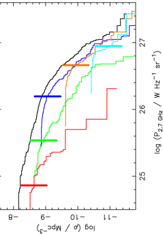
Figure 4: The integral radio luminosity function for the QSOs of the Parkes 0.25-Jy flat-spectrum sample, computed in the five redshift ranges of Fig. 3: $0-0.5$ (red), $0.5-1.0$ (green), $1.0-2.0$ (blue), $2.0-3.0$ (orange) and $3.0-5.0$ (light blue). Vertical lines again indicate limits of completeness for each redshift range, due to spectral-index spread. The upper curve is the total integrated luminosity function, complete for all powers only at the very highest luminosities.

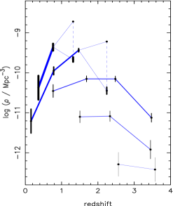
Figure 5: Space densities as a function of redshift for 5 power ranges, log$P_{2.7}=25.8-26.2$, $26.2-26.6$, $26.6-27.0$, $27.0-27.4$, and $27.4-27.8$, denoted by decreasing line weight. Abscissa values are the mean redshifts in each element of ($\Delta P_{2.7}$, $\Delta z$). For each of the two lowest power ranges, the final point with error bar represents incomplete data, as these points fall at powers below the spectral cutoffs shown in Fig. 3. Upper limits, represented by the single dots, were obtained by extrapolating the RLF to this power from higher powers. The actual values therefore lie somewhere along the two dashed lines.

4 The Redshift Cutoff

Our preliminary analysis (Shaver et al. 1996) indicated a decrease in radio-QSO space density beyond $z=3$. Using a well-defined sub-sample from the present study, Shaver et al. considered the space density of QSOs with $P_{\rm 2.7\,GHz}\geq 1.1\times 10^{27}$ W Hz^-1 sr^-1. On the basis of uniform space density, the 25 such radio QSOs seen at $z\leq 4$ indicate that 15 similar objects would be expected in the range $5\leq z\leq 7$. None was found. From Poisson statistics, the difference is significant at the 99.9% level.

This preliminary study drew attention to a possible difficulty in the analysis due to the curved nature of some of the radio spectra. Jarvis & Rawlings (2000) examined this in some detail, pointing out the apparently curved nature of many of the radio spectra involved, and indicating how such an effect, a steepening to the high frequencies in particular, might reduce or remove the significance of an apparent redshift cutoff. Their model-dependent analysis used only the highest-power objects and indicated that the apparent cutoff on the basis of such objects might have a significance level as low as that corresponding to $2\sigma$. They suggested that establishing the reality of the cutoff for such objects to a high level of significance might be difficult even with all-sky samples. However, Fig. 6 shows that there is no clear majority of sources with spectra steepening to the higher frequencies. Moreover, we show below that the spectral data in the literature are misleading in terms of the proportion of sources showing spectral steepening to the higher frequencies.

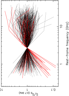
Figure 6: The radio spectra of all sources in Sample 2, Table 2, in their rest frame. Data are at observing frequencies of 0.365, 1.4, 2.7, 5.0, 8.40 and 8.87 GHz, and flux densities are normalized by $S_{0}$, the interpolated rest-frame flux density at 2.7 GHz. The red lines represent the brightest sources, those with $S_{\rm 2.7\,GHz}\geq 2.0$ Jy.

Subsequently we have considered alternative methods to study space density and redshift distribution, methods to utilize the entire sample which can demonstrate simple attributes of the space-distribution without recourse to modelling the luminosity function or its epoch dependence.

4.1 The Power-Volume plane; using the whole sample

Fig. 7 (left) shows sources of Sample 3 (Table 2) in a plot of radio luminosity vs. co-moving volume. We need this new sample for such a plot. Recall that Sample 1 (Table 1) included all sources, not just QSOs, while Sample 2 (Table 2), although confined to QSOs, was drawn from regions of the survey with different completeness limits. In order for a plot of luminosity vs. $z$ (or equivalently, co-moving volume) to be interpreted, the sample must have a single survey limit. Sample 3 is therefore composed of all QSOs from our data table of Paper 1 with survey completeness limit at exactly $S_{\rm 2.7\leavevmode\nobreak\ GHz}=0.25$ Jy (Fig. 1, Paper 1), and again at declinations above $-40\hbox{${}^{\circ}$}$ for reasons of radio-spectral completeness. Fig. 7 shows lines of survey completeness corresponding to 0.25 Jy for three different radio spectral indices.

The plot with co-moving volume on the abscissa rather than redshift gives direct indication of space density. There is an apparent diminution in the density of points at redshifts above $\sim 2.5$. The question is whether this is real and significant. In what follows we test the null hypothesis that the space density of QSOs at high redshifts remains constant and equal to that at $1<z<3$.

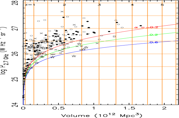
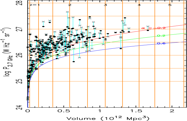
Figure 7: The Luminosity - Volume plane for the 252 QSOs with measured redshifts, in survey areas with completeness limit $S_{\rm 2.7\,GHz}=0.25$ Jy (Sample 3, Table 2). Vertical grid lines indicate redshifts, as marked along the top border. The curved lines indicate survey completeness limits at 0.25 Jy for three spectral indices. Left: the sources plotted with symbols to indicate different spectral indices $\alpha^{2.7}_{5.0{\rm GHz}}$: solid dots for $-0.4<\alpha<-0.2$; open circles for $-0.2<\alpha<+0.2$, crosses for $+0.2<\alpha<+0.6$, and stars for the extreme spectral inversions $\alpha>+0.6$. Rest-frame luminosities ($P_{2.7}$) for this plot were calculated assuming a power-law spectrum given by this index. Note that the dots lie above the $\alpha=-0.2$ limit line; the open circles above the $+0.2$ line; the crosses above the $+0.6$ line; and the stars scatter to below the $+0.6$ line. Right: The effects of considering spectral data at frequencies below the Parkes survey frequency (2.7 GHz). The values of $P_{2.7}$ are substantially changed. Crosses indicate the original positions as in the left panel, while dots show the positions revised with improved estimates due to incorporation of lower-frequency data.

Redshift information is not complete for Sample 3; in order to make comparison with prediction we must estimate the number of possible objects at $z>3$. Table 2 presents the summary. The key element is the sub-sample of 16 objects in the sample of 268 for which redshifts are not available.

The redshift distribution for QSOs is known to be a function of both apparent magnitude and flux density, albeit with huge scatter and only a gentle dependence in each case. Thus in order to estimate redshift proportions for the objects without such data, we treated the identifications made on UKST plates and those from the (deeper) CCD observations separately.

Consider the 11 QSOs without redshifts and identified from UKST plates. Of the 242 objects identified on UKST plates and with measured redshifts, 8 have $z>3$. There is no bias in the redshift measurements or lack of; and thus we expect $8/242\times 11=0.36$ of the 11 objects to have $z>3$. The remaining 5 objects may be treated equally; the single unidentified source in the sample (PKS 0225-065) escaped the CCD identification programme by being de-identified later on the basis of an improved radio position. Had it been included we can be confident that an identification would have been obtained, as it was in each of the 87 cases we tried. For these 5 objects, then, we use the CCD-identified QSOs with redshifts, totalling 10 in the sample, for which two redshifts exceeded 3. We thus anticipate $2/10\times 5=1.0$ of the 5 objects will have $z>3$. The number of objects in the sample with measured $z>3$ is 10. Thus the number with which to compare predictions for $z>3$ is $10$(observed)$+1.4$(estimated)$=11.4$. The principal point is that redshift incompleteness does not impede our analysis.

A simple analysis may be carried through on the basis of Fig. 7. If we consider QSOs in specific narrow bins of luminosity and survey limit imposed by spectral index and survey flux limit $S_{\rm lim}$, then such horizontal stripes in Fig. 7 intersecting the curved survey-cutoff lines provide an area in the figure in which QSOs can be seen by the survey. On the null hypothesis, no redshift diminution, if we now split this area into a region with $z<3$ and a region with $z>3$, we can use the surface density of QSOs in the low-redshift area to form an expectation value for the higher redshift area. We chose the prediction region to be $1<z<3$ to coincide roughly with the plateau of the ‘quasar epoch’, and we selected the high-redshift region to run out to $z=8$, the approximate limit to which we could hope to see QSOs given our survey limits and the known range of luminosity and spectral index.

This process described above can be refined by reducing the stripes of radio power to zero width; each source then becomes a predictor, provided of course that the survey limit allows it to be seen beyond a redshift of 3. Table 4 presents results of this analysis under the sub-heading ‘single survey cutoff’. The immediate result is the apparent one: a prediction of significantly more QSOs at $z>3$ than the 11.4 ‘seen’.

Table 4: Predicted numbers of QSOs, $3<z<8$

Sample	Observed at $z>3$	Analysis type	Contributors	Predicted${}^{\dagger}\leavevmode\nobreak\ 3<z<8$
Single survey cutoff:
3	11.4	single cutoff, $\alpha=+0.2$	73(86)	64.7(66.7)
3	11.4	single cutoff, $\alpha=\ \ 0.0$	49(57)	40.3(40.4)
3	11.4	single cutoff, $\alpha=-0.2$	39(43)	25.0(25.1)
Source-by-source analysis, ‘Single-source survey’:
2	17.8	$S_{2.7},S_{5.0}$	71(89)	51.5(53.5)
2	17.8	$S_{0.365},S_{1.40},S_{2.7},S_{5.0}$	67(89)	48.5(54.0)
2	17.8	$S_{0.365},S_{1.40},S_{2.7},S_{5.0},S_{8.40}$	53(65)	28.8(30.1)
2	17.8	$S_{0.365},S_{1.40},S_{2.7},S_{5.0},S_{8.87}$ or $S_{8.40}$	57(70)	38.6(38.6)
2	17.8	$S_{0.365},S_{1.40},S_{2.7},S_{5.0},S_{8.87}$	70(88)	50.5(52.9)

^†calculated in the geometry adopted for this paper; bracketed numbers are for $\Omega_{\rm m}=\Omega_{\rm tot}=1.0$, the Einstein - de Sitter Universe

The results reveal a fundamental flaw of this analysis, namely what limit line to adopt, corresponding to which spectral index. It is apparent from Fig. 7 that adopting $\alpha=-0.2$ is extreme; but even confining the analysis to narrow bands of spectral index does not define where within that band the survey cutoff or completeness line should be placed. The analysis at this point appears to confirm what the eye sees in Fig. 7, but shows that taking the figure at face value is dangerous. Moreover here we have used the $2.7-5.0$ GHz spectral index, characterizing each spectrum as a single power law; spectral curvature or indeed any complexity of radio spectrum has not been considered. (For low-frequency surveys, the spectral-index issue is not so important, because most sources detected in them have power-law spectra characterized by an index close to $-0.75$. In corresponding $P-z$ or $P-V$ planes, most sources from low-frequency surveys cluster closely along or just to the left of the single limit line given by this spectral index.)

The analysis of Shaver et al. (1996) attempted to circumvent the difficulties by sticking to powers so high that the observational cutoff, the survey completeness limit, did not come in to play. In doing so, the available sub-sample becomes small and the statistical uncertainties are inevitably larger.

These difficulties suggest the following refinement.

4.2 Source-by-source analysis: the ‘Single-Source Survey’

There is no need to stick to a single survey-limit line in the $P-V$ plane. Each source can be considered alone, conceptually the result of a survey which found it as a single source. For each such ‘single-source survey’, a limit line may be drawn in the plane peculiar to that object and incorporating all its radio-spectral information. The prediction of this object for sources at redshifts above 3 may then be added to the predictions from all ‘single-source surveys’ to derive a prediction total. In effect this is using the $V_{\rm max}$ method to predict the number of objects in volumes at higher redshift on the hypothesis that space density is uniform; it is doing so using the spectral properties of each source individually.

A further advantage in such a process is that there is no longer a need to stick to a sample defined by a single flux-density limit. To improve statistical weight, all zones of the survey can be used, no matter what the flux-density limit, provided of course that the value of the 2.7-GHz flux density is greater than or equal to the completeness limit for the area in which it was detected. (Sources for which this is not the case were marked in the data-table of Paper 1.) Each source in this analysis contributes a predicted number of sources given by the ratio of its accessible co-moving volume in the redshift range $3<z<8$ to that in the range $1<z<3$. The sum of all such predicted sources, based on all sources observed in the redshift range $1<z<3$, gives us the total number of $3<z<8$ sources expected in the survey for a constant comoving space density.

A sample appropriate to this analysis is Sample 2 of Table 2, giving a total of 379 radio QSOs, 355 with measured redshifts. From an analysis analogous to that carried out for Sample 3, we estimate that complete identification and redshift data would add 1.8 sources to the 16 members of this sample observed to have $z>3$.

As a basic analysis of this type, when individual limits are applied as described, using the $\alpha^{5.0}_{\rm 2.7\,GHz}$ spectral index appropriate to each source, a prediction of 51.5 sources in the redshift range $3<z<8$ is obtained (Table 4), c.f. the 17.8 sources ‘observed’. However a particularly important feature of the approach is that it enables incorporation of all radio spectral data. Other investigators (in particular Jarvis & Rawlings 2000) have emphasized how important the form of the spectrum is. As mentioned in the previous section, there are several effects on space density analysis and these are illustrated in Figs. 7 and 8:

1. If the spectrum decreases to low frequencies, perhaps having a low-frequency cutoff due to synchrotron or free-free absorption, the effective power at the rest-frame survey frequency is reduced. The result may be a substantially lower position in the $P-V$ plane. This reduces the ‘headroom’ the object has to predict significant contribution at higher redshift; and it may remove it from the ‘prediction contributors’ list entirely. Significant steepening to the lower frequencies of course has the opposite effect, raising its rest-frame power, its position in the $P-V$ plane, and increasing its prediction.

   We have incorporated spectral data at 1.4 GHz from the NVSS survey (Condon et al. 1998) and at 0.365 GHz from the Texas Survey (Douglas et al. 1996) to define the low-frequency spectra for the majority of sources in Samples 2 and 3. The results may be seen in Fig. 7. The extreme-power objects have convex spectra and drop down into the pack; but in addition, a number of less-luminous objects rise by virtue of steep low-frequency spectra. When the prediction is made incorporating the low-frequency data (Table 4), these effects approximately cancel out and the result differs little from the previous estimate: 48.5 objects should be seen in the sample at $3<z<8$, c.f. the ‘observed’ number of 17.8.

2. A more substantial difference is produced by the incorporation of spectral data at frequencies higher than 5.0 GHz. Shaver et al. (1996) pointed out that high-frequency flux densities measured quasi-simultaneously by Gear et al. (1994) indicated little spectral steepening; and certainly not enough to exclude very-high-redshift objects. However the Gear et al. (1994) sample may not be representative. For PKS sources a set of flux densities at 8.4 GHz was measured by Wright et al. (1990), including a large fraction of the sources in both Sample 2 and Sample 3. These data suggest that spectral steepening is more common than indicated by the Gear et al. (1994) measurements, although as Fig. 6 shows, it is not a feature of the majority of sources.

   Spectral steepening beyond 5 GHz in the observer frame has two effects. First it moves the cutoff line upward (Fig. 7) so that the object in question drops from the sample at relatively lower redshifts. Secondly when ‘moving’ the object to some redshift above the observed redshift, the spectrum becomes steeper than the apparent 2.7 – 5.0-GHz spectral limit of $-0.4$ used to define the original sample; ‘flat-spectrum’ objects whose spectra steepen beyond 5.0 GHz (observer frame) become undetected as such at higher redshifts.

   To consider the first of these two effects, the cutoff (survey limit) line for each source was calculated using each ‘segment’ of the spectrum as redshift is changed. This simple interpolation in the log $S_{\nu}$ - log $\nu$ plane results in segmented cutoff lines for each object in the $P-V$ plane as shown in Fig. 8.

   

   

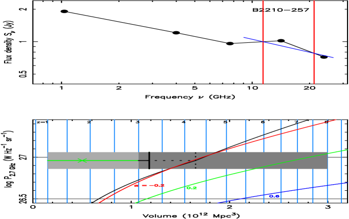
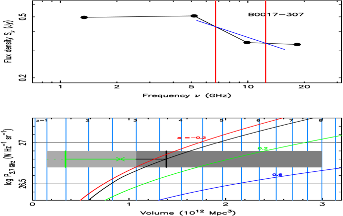
   Figure 8: Two sources to illustrate redshift limits in the single-source analysis. For each object, the upper panel shows the spectrum in the rest frame, while the lower panel shows the object in the $P-V$ plane. In each case the individual cutoff lines are shown as the segmented black curves in the $P-V$ plane, while the smooth coloured curves represent completeness limits at $S_{\rm 2.7\,GHz}=0.25$ Jy for sources whose spectra are described by single power laws with indices as shown. Light grey bars represent the predictive region $1\leq z\leq 3$, dark grey the region $3\leq z\leq 8$ in which the object might be visible; the width of these bars is irrelevant. In the case of PKS 2210-257, the individual survey limit suggests that the object should be visible out to z=4.54. However, it is not visible to this redshift as an object with an observed 2.7 - 5.0 GHz spectrum flatter than $-0.4$; the spectrum (shown blue) steepens to an effective index of $\leq-0.4$ at a redshift of 3.22, for which the ‘observed’ frequencies of 2.7 and 5.0 GHz are shown in the upper panel by the red vertical lines. The object therefore drops from the sample at this redshift. PKS 0017-307 does not enter the observed region of the diagram as an object with spectral index $\geq-0.4$ until a redshift of 1.48 is reached. Again in its upper panel, the red vertical lines indicate rest frequencies at 2.7 and 5.0 GHz for the critical redshift of 1.48, at which point the spectrum ‘flattens’ to have $\alpha\geq-0.4$, denoted by the blue line. The object runs into its observable limit at z = 3.60 in the predictive region as shown. The smaller accessible volume in the ‘observed’ region results in a scaling up of its prediction via the ratio of accessible volumes.

   The second of these two effects is illustrated by PKS 2210-257 in the left-most panel of Fig. 8. As the effective spectrum steepens with increasing redshift, the accessible region in the redshift range $3<z<8$ is reduced substantially from that given by the power cutoff line. The prediction from such an object reduces correspondingly.

3. There is a third effect due to spectral measurement affecting the ‘observed’ region $1<z<3$, if the spectrum steepens at frequencies below the survey frequency. The effect is illustrated in the right panel of Fig. 8: objects such as PKS 0017$-$307 are invisible to us as ‘flat-spectrum’ sources at redshifts below a cutoff point at which the upward curvature makes them appear ‘steep-spectrum’. This affects only a few sources, but for these, it means an increase in prediction contribution calculated as the ratio of (accessible volume $3<z<8$)/(accessible volume $1<z<3$).

When the available spectral measurements, relatively complete for Sample 2 at five frequencies, are considered for each source, the prediction (Table 4) is 28.8 sources, differing now from the ‘observed’ number 17.8 by just 2.9$\sigma$. The raised level of the power cutoff does most of the damage. It is this use of the data for the Parkes 0.5-Jy sample which we believe yields the relatively low level of significance for a redshift cutoff found by Jarvis & Rawlings (2000).

However there is a fundamental problem with using the 8.40-GHz data. This can be shown by using a set of 8.87-GHz flux densities measured in 1972 (Shimmins & Wall 1973), roughly contemporaneous with the 2.7-GHz surveys. There are 40 sources in Sample 2 with these ‘old’ measurements, one of which, PKS 1532+016 at $S_{\rm 8.87\,GHz}=1.16$ Jy, was not measured by Wright et al. (1990). There are clearly large flux-density variations at 8 GHz, the wildest being for PKS 1402$-$012, 0.67 Jy in 1972, 0.15 Jy in 1989. If the 1972 8.87-GHz measurements are used in preference to the 1989 8.40-GHz measurements, the prediction is 38.6 QSOs (57 contributors) in the range $3\leavevmode\nobreak\ <\leavevmode\nobreak\ z\leavevmode\nobreak\ <\leavevmode\nobreak\ 8$. This is very significantly higher than the prediction of 28.8 (53) sources using only 8.40-GHz data, exceeding the 17.8 sources ‘observed’ by 4.9$\sigma$.

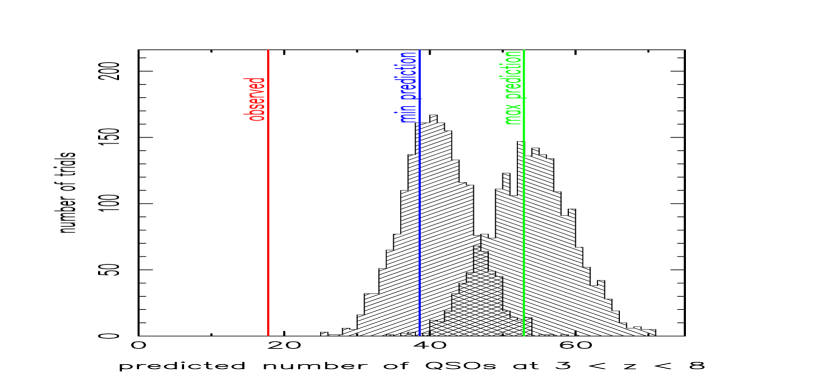
Figure 9: The predicted numbers of QSOs at high redshifts. The histograms are the results of 2000 trials of end-to-end bootstrap testing. The left-most histogram was compiled using high-frequency spectral data at 8.40 GHz and 8.87 GHz, with the 8.87-GHz (near-contemporary) flux densities used in preference if both were available. The right histogram represents 2000 results from bootstrap testing when only the 8.87-GHz flux densities were used. The vertical line to the left indicates the observed number of QSOs at high redshifts, as discussed in the text. These bootstrap test were carried out in the simple geometry $\Omega_{\rm m}=\Omega_{\rm tot}=1$ but are closely indicative of results for the $\Lambda$ - dominated geometry adopted here (see Table 4 and text).

The problem is a simple one. Measuring high-frequency flux densities some time after the original survey gives a biased estimate of the spectrum. Any flux-limited survey preferentially selects variable sources in an up-state, whereas flux-density measurements many years later reflect sources in a mean state. The result is that the spectra are artificially steepened. In the present case the result is an underestimate of numbers of objects predicted at high redshifts. It is the variations at frequencies above the survey frequency which matter in this; variations at the lower frequencies are small to insignificant in comparison.

The result emphasizes how responsive the predictions are to flux measurements, and how crucial it is to use contemporaneous measurements. If this much change comes about with replacing the 8-GHz flux densities of just 40 sources with near-contemporary measurements, it is certain that the prediction of 38.6 sources based on using all the remaining (non-contemporary) 8.40-GHz flux densities represents an underestimate or lower limit. If the 8.40-GHz flux densities are ignored and only the 8.87-GHz data used as flux densities at frequencies above 5.0 GHz, the result is a prediction of 50.5 sources. This must be an overestimate. The 8.87-GHz flux densities were measured preferentially for bright sources at high frequencies, and thus favour objects well above survey-limit lines. We conclude that on the hypothesis of uniform space distribution, somewhere between 38.6 and 50.5 sources are predicted to have redshifts between 3 and 8 for Sample 2.

To assess the uncertainties an end-to-end bootstrap experiment was run for the two possibilities: (i) using as high frequency data only the 8.87-GHz (1972) measurements, and (ii) using the combination of 8.87 and 8.40-GHz measurements, with the former taking precedence if measurements at both flux densities were available. Because of computing time constraints we had to run this experiment using the simple geometry of $\Omega_{\rm tot}=\Omega_{\rm m}=1$. However as Table 4 shows, the predictions in this geometry are very similar to the predictions of the $\Lambda$ - dominated cosmology, the numbers in question being 38.6 and 52.9 for the simple geometry vs. 38.6 and 50.5 for the $\Lambda$ - dominated geometry. The uncertainties should be representative. In the bootstrap sampling, random redshifts were assigned to each source from the total sample of redshifts. The flux densities for the source were then ‘corrected’ to that particular redshift making use of the measured redshift of the object. The results are shown in Fig. 9. Some 2000 trials for each of the two possibilities produced no prediction as low as the ‘observed’ number of 17.8 QSOs at $z>3$.

There are two results from this analysis:

1. The true prediction of numbers of QSOs at $3<z<8$ for a uniformly-filled universe lies between 38.6 and 50.5 objects for Sample 2. This is to be compared to the ‘observed’ number of 17.8. An end-to-end bootstrap test indicates that the difference is highly significant.

2. High-frequency flux-density measurements that are non-contemporary are dangerous. They bias the spectral statistics of any variable-flux sample, because surveys pick out variable sources in their high state, and not in their average state.

5 The form of the evolution

Figs. 3 and 5 indicate that the form of the evolution, and in particular the shape of the decline at high redshifts, cannot be inferred directly. As an indirect route, we used Sample 2 and proceeded as follows:

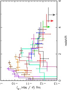
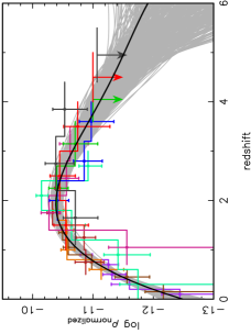
Figure 10: Above: space density $\rho$ vs redshift. The individual RLFs are each complete from $z=1.0$ to $z=5.5$ in steps of $\Delta z=0.5$, in the order purple, brown, orange, dark red, light blue, turquoise, blue, green, red, grey. Below: these RLFs normalized to agree over the range at $1.0<z<2.5$. The bold black line is a least-squares fit with a polynomial of fifth order, given in the text. The grey lines represent 1000 bootstrap trials. In this process, fits which resulted in lines of positive slope beyond $z=5$ were rejected.

1. Ten redshift limits were set up, from $z_{l}=1.0$ to $z_{l}=5.5$ in steps of $\Delta z=0.5$. We then determined the combination of $P_{2.7}$ and effective spectral index yielding the maximum number of contributors to the RLF for the sub-sample complete to each of these redshift limits. The numbers of RLF contributors in these complete sub-samples ranged from 285 at $z=1.0$ down to just 9 at $z=5.5$; the numbers decrease since higher luminosities are needed to be complete to the larger redshift limits.

2. For each of these 10 sub-samples, we computed the RLF using the $1/V_{\rm max}$ contributions already calculated for previous estimates of luminosity functions. For the two samples with redshift limits at 5.0 and 5.5, there are no sources in the upper bins, and to use this observation we assigned an upper limit of one source to each of them. The results are shown in Figure 10, upper panel.

3. Although these RLFs are each now complete from $z=0$ to $z=z_{l}$, individually they are inadequate to trace the whole QSO epoch. Those with smaller values of $z_{l}$ by definition cannot reach large redshifts, while those with the larger $z_{l}$ are severely noise limited, particularly at the low-redshift ends. To combine these results to define the overall space behaviour, we normalized each curve to agree statistically over the range $1.0<z<2.5$. We then fitted a least-squares polynomial through the points, with the results shown in the lower panel of Fig. 10. The heavy black line in this diagram is

   $${\rm log}\rho=-12.49+2.704z-1.145z^{2}+0.1796z^{3}-0.01019z^{4}.$$

4. Finally a constrained bootstrap experiment of 1000 runs was used to give an approximation to the uncertainty; the grey area in the figure is the result.

Normalizing as described is only valid if the form of evolution is independent of radio luminosity. There is some indication in the data (Fig. 10, upper panel) that the turnovers set in at redshifts increasing with luminosity. If so, then normalizing as described would broaden the maximum, and the overall curve would be representative of the overall evolution form, but in no sense formally accurate. Moreover, the complete individual pieces of luminosity function are not statistically independent, so that the shaded area is indicative of uncertainty, but again is not accurate in a formal sense.

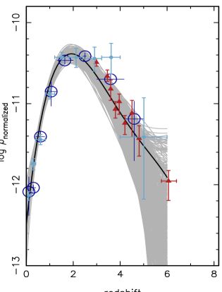
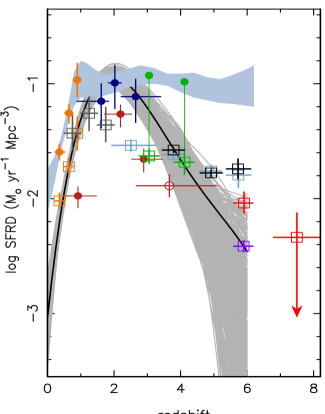
Figure 11: Left: Relative space density of QSOs ($\rho$) as a function of redshift. The shaded area and black line represent the current QSO space-density determination from Figure 10. Light blue filled circles show the soft X-ray data from Chandra and XMM-Newton surveys (Hasinger et al. 2004), while the dark blue open circles show the results from combined Chandra and ROSAT surveys (Silverman et al. 2004). Space density behaviour of optically-selected QSOs is given by the set of dark red triangles; the data are from Schmidt et al. (1995), Fan et al. (2001b) and Fan et al. (2004). The point at $z\sim 6$ is taken from Fan et al. (2004) and due to conversion between geometries there is uncertainty in the ordinate of $0.1$. The X-ray and optical QSO data were scaled vertically to match the current determination of space density at redshifts 2 to 2.5. Right: Star formation rate density (SFRD; units adopted by Blain et al. 2002), with the shaded area and black line again showing the current estimate of radio QSO space density. Data in optical and near-IR bands are distinguished as squares: orange (Lilly et al. 1996), grey (Connolly et al. 1997), green (Steidel et al. 1999), light blue (Bouwens et al. 2004a), black (Giavalisco et al. 2004), purple (Bunker et al. 2004) and red (Bouwens et al. 2004b). In general these data have not been corrected for extinction. Green dots show results of the extinction correction of 4.7 suggested by Steidel et al. (1999) for their data; the light blue band represents an estimate of the SFR determined from these and other points as analyzed by Bouwens et al. (2004b). Measurements from Far-IR and sub-mm observations are shown as circles: FIR as orange filled circles from Flores et al. (1999), and sub-mm as dark red filled and open circles and blue filled circles from Bouwens et al. (2004b), discussed in the text. The current space density determination (black curve) was scaled to match the Lilly et al. (1996) points, the orange open squares.

These results enable comparison with other high-redshift observations. Fig. 11 shows the shaded area of Fig. 10 in the background, with data from recent compilations of space density as a function of redshift for AGNs selected at X-ray and optical wavelengths (left panel), and star-formation rate (SFR) as a function of redshift (right panel).

Agreement with the form of the X-ray-selected QSO evolution is remarkably good. Silverman et al. (2004) found the X-ray decline to agree in form with the optical decline determined by Fan and co-workers (Fan et al. 2001a, c, b) from SDSS. Silverman et al. also showed that the COMBO-17 survey results of Wolf et al. (2003) follow the X-ray data closely. The Hasinger et al. (2004) X-ray AGN results are again in very good agreement with the current determination. There is thus general accord between the dependence of space density for QSOs found at radio, optical and X-ray wavelengths, all showing a rapid rise in co-moving space density to $z\sim 1.5$ followed by declining space densities at $z>3$. However, there are strong dependencies of evolution form on luminosity, certainly for the optical and X-ray samples as noted by Hasinger et al. (2004) and Silverman et al. (2004); and there may be such dependence for the current radio-selected sample. The dependence on luminosity is well illustrated by the fact that the rising curve of (lower-optical-luminosity) QSOs selected from the 2dF survey (Croom et al. 2004) is displaced to higher redshifts than the X-ray or radio-selected QSOs. The current agreements are illustrative only; analysis of the significance must await larger samples providing better definition of space density evolution as a function of luminosity in each wavelength band.

The relation between QSO space evolution and star-formation-rate history is not so clear. The general similarity was first noted in 1997 (Wall 1998); the rise to redshifts of $\sim 1.5$ appears to be of the same form. But at this redshift it appears that determinations of the SFR from UV, optical and near-IR measures produce a different form of epoch dependence, with an abrupt transition to a law almost constant (or diminishing gradually) with increasing redshift out to $z>6$. There are substantial uncertainties in what extinction correction to apply; but this form appears to hold whether or not the data are extinction-corrected (provided as claimed that the correction is not strongly dependent on redshift). The open squares of Fig. 11, uncorrected for extinction, show the gradual decline, while the band (Chapman et al. 2004), representing a fit to extinction-corrected data, shows a star formation rate essentially independent of redshift to $z>6$. The data from sub-mm observations (dark blue and red circles, filled and open; Chapman et al. 2004) represent estimates from radio-identified sub-mm galaxies (red circles), and from these galaxies and sub-mm galaxies combined (blue circles). Chapman et al. point out that the similarity of star-formation-rate contributions at $z\sim 2$ suggests that the total SFR from all populations may exceed the current estimates significantly.

It remains somewhat puzzling that the sub-mm galaxy star-formation-rate appears to drop beyond $z=3$, and that it therefore resembles the AGN space-density law rather than that of the galaxies detected in the optical and near-IR. This may be superficial, in that the points are lower limits, and additional components may be found. It is perhaps less puzzling that the AGN space-density law differs from the overall SFRD in the sense observed. On current hierarchical pictures, redshifts beyond 3 represent the era of rapid galaxy assembly; and there may be a delay before the large enough galaxies have developed to host massive black holes, or before the galaxy-building process provides orbit organization appropriate to fuel such black holes.

6 Summary

We summarize the results of this and the preceding two papers (Jackson et al. 2002; Hook et al. 2003).

1. (Paper 1) The initial goal of the project was to search for high-redshift QSOs without dust bias. Optical counterparts for essentially all flat-spectrum objects in the sample were obtained. No QSOs at redshifts greater than 5 were found.

2. At the fainter flux densities ($S_{2.7}<0.4$ Jy) and optical magnitudes ($B_{J}>20.0$), substantial numbers of flat-spectrum radio galaxies are present (Paper 1, Fig. 7). These may have influenced previous claims for a hidden population of heavily-reddened QSOs; ‘red’ QSOs (Rieke et al. 1979) do not appear to constitute a major fraction of the total population sampled here. Amongst the reddest of the stellar identifications, about one-quarter are BL Lac objects, compared to 9 per cent with no colour selection, supporting the synchrotron interpretation for many of the red objects originally proposed by Rieke et al. (1979). However, the discovery of molecular line emission from a sample of the redder QSOs by Carilli et al. (1998) indicates the likely presence of dust in some systems, possibly concentrated in dense nuclear tori.

3. (Paper 2) A composite optical spectrum for flat-spectrum QSOs derived from the present sample shows clear qualitative differences in comparison with radio-quiet composite spectra: the Ly-$\alpha$(1216Å) and CIV(1549Å) lines are stronger in the current sample. There appears to be no significant difference in the Ly-$\alpha$ decrement between radio-loud and radio-quiet QSOs.

4. (Present paper) The redshift distribution has been derived for the quarter-Jansky sample, with consideration given to the different constituents - red galaxies, BL Lac objects and QSOs. Comparison with the space-density models of Dunlop & Peacock (1990) and Jackson & Wall (1999) indicates substantial agreement, although refinement of space-density modelling is clearly possible using the current data.

5. Radio luminosity functions for flat-spectrum QSOs have been calculated using the $1/V_{\rm obs}$ method. These show the rapid increase in space density between $z=0$ and $z=1$, a flattening between $z=1$ and $z=2.5$, and evidence of declining space density to yet higher redshifts. Attention is drawn to a selection effect producing an apparent flattening of the luminosity functions towards lower powers in each redshift shell. This effect, due to intrinsic spread in radio spectra, may have gone unrecognized in previous analyses, leading to overinterpretation of similarities in form of the RLF at each redshift.

6. The reality of a redshift cutoff has been verified using the ‘single-source survey’ $V_{\rm max}$ method, in which each QSO in the sample is used to predict the number of sources observable at higher redshifts on the assumption of uniform space density. The technique is robust and model-free, and it makes use of all QSOs in the sample, rather than limiting the statistics to the few objects of highest radio luminosity.

7. The result of this analysis has been to demonstrate that a space-density diminution exists at $z>3$, at significance levels of $>4\sigma$. Precise significance cannot be evaluated, because it is shown that spectral data at high frequencies are critical, and that non-contemporary flux-density measurements seriously bias the results towards reducing the apparent redshift diminution.

8. In the light of this high-redshift diminution, an estimate has been made of the overall evolution for the radio-loud QSO population. The model-free approach has been retained, with the form mapped simply by fitting a least-squares polynomial to the data. This was followed by a bootstrap analysis - 1000 more polynomial fits - to provide an indication of the uncertainty.

9. The form of this evolution was compared with that determined for X-ray QSOs (Chandra, XMM-Newton and ROSAT results) and for optically-selected QSOs (primarily SDSS results). Agreement is excellent. It was further compared with the evolution of star formation rate. Current best estimates of this from optical and near-IR data show that although the initial rise may be of similar form, there is divergence at redshifts beyond 1.5. While the AGN space density dives down at $z>3$, the SFR appears shows relatively little dependence on redshift to $z>6$. The picture from sub-mm measurements is less clear. Uncertainties are large, but the SFR determined from sub-mm data appears curiously to follow the AGN relation more closely than it follows the SFR law found from galaxies detected with optical and near-IR measurements.

10. In view of the diminution in space density to high redshifts, radio-loud QSOs would appear to have little role to play in the reionization epoch $6<z<17$.

The reality of the redshift cutoff for radio-selected QSOs and its similarity with that observed for optically-selected QSOs leads to the conclusion that the apparent cutoff for the latter is real and is not due to dust. This conclusion is consistent with the results from the CORALS survey (Ellison et al. 2001, 2002), in which a complete sub-sample of radio-selected QSOs from the Parkes quarter-Jansky sample was searched for damped Ly-$\alpha$ (DLA) systems. Little significant difference for the comoving mass density of neutral gas was found between the estimate from the CORALS sample and those from previous (optically selected) samples. No major population of high-column-density absorbers has been missed. Our view of the high-redshift diminution of the QSO population does not appear to be dominated either by intrinsically dusty systems or by a major Universal dust screen.

Acknowledgements. We are very grateful to Matt Jarvis and Steve Rawlings for a helpful dispute. We thank Greg Bryan, Xiaohui Fan, Charles Jenkins, Anna Sajina and Douglas Scott for valuable discussions. We are grateful to Günther Hasinger and colleagues for providing us with data and results prior to publication. The National Radio Astronomy Observatory is operated by Associated Universities, Inc. under a cooperative agreement with the U.S. National Science Foundation.

References

- Avni & Bahcall (1980) Avni, Y. & Bahcall, J. N. 1980, ApJ, 235, 694
- Barger et al. (2003) Barger, A. J., Cowie, L. L., Capak, P., et al. 2003, ApJL, 584, L61
- Becker et al. (2001) Becker, R. H., Fan, X., White, R. L., et al. 2001, AJ, 122, 2850
- Bennett et al. (2003) Bennett, C. L., Hill, R. S., Hinshaw, G., et al. 2003, ApJS, 148, 97
- Blain et al. (2002) Blain, A. W., Smail, I., Ivison, R. J., Kneib, J.-P., & Frayer, D. T. 2002, Phys. Rep., 369, 111
- Bouwens et al. (2004a) Bouwens, R. J., Illingworth, G. D., Thompson, R. I., et al. 2004a, ApJL, 606, L25
- Bouwens et al. (2004b) Bouwens, R. J., Thompson, R. I., Illingworth, G. D., et al. 2004b, astro-ph/0409488
- Boyle et al. (1991) Boyle, B. J., Jones, L. R., Shanks, T., et al. 1991, in ASP Conf. Ser. 21: The Space Distribution of Quasars, Ed Crampton, D., 191
- Boyle et al. (1988) Boyle, B. J., Shanks, T., & Peterson, B. A. 1988, MNRAS, 235, 935
- Boyle & Terlevich (1998) Boyle, B. J. & Terlevich, R. J. 1998, MNRAS, 293, L49
- Bunker et al. (2004) Bunker, A. J., Stanway, E. R., Ellis, R. S., & McMahon, R. G. 2004, MNRAS, 450
- Carilli et al. (1998) Carilli, C. L., Menten, K. M., Reid, M. J., Rupen, M. P., & Yun, M. S. 1998, ApJ, 494, 175
- Cen & McDonald (2002) Cen, R. & McDonald, P. 2002, ApJ, 570, 457
- Chapman et al. (2004) Chapman, S., Smail, I., Blain, A., & Ivison, R. 2004, astro-ph/0406596
- Condon et al. (1998) Condon, J. J., Cotton, W. D., Greisen, E. W., et al. 1998, AJ, 115, 1693
- Connolly et al. (1997) Connolly, A. J., Szalay, A. S., Dickinson, M., Subbarao, M. U., & Brunner, R. J. 1997, ApJL, 486, L11
- Croom et al. (2004) Croom, S. M., Smith, R. J., Boyle, B. J., et al. 2004, MNRAS, 349, 1397
- Douglas et al. (1996) Douglas, J. N., Bash, F. N., Bozyan, F. A., Torrence, G. W., & Wolfe, C. 1996, AJ, 111, 1945
- Dunlop & Peacock (1990) Dunlop, J. S. & Peacock, J. A. 1990, MNRAS, 247, 19
- Ellis (1999) Ellis, R. S. 1999, Ap&SS, 267, 319
- Ellison et al. (2001) Ellison, S. L., Yan, L., Hook, I. M., et al. 2001, A&A, 379, 393
- Ellison et al. (2002) Ellison, S. L., Yan, L., Hook, I. M., et al. 2002, A&A, 383, 91
- Fall & Pei (1993) Fall, S. M. & Pei, Y. C. 1993, ApJ, 402, 479
- Fan et al. (2004) Fan, X., Hennawi, J. F., Richards, G. T., et al. 2004, AJ, 128, 515
- Fan et al. (2001a) Fan, X., Narayanan, V. K., Lupton, R. H., et al. 2001a, AJ, 122, 2833
- Fan et al. (2002) Fan, X., Narayanan, V. K., Strauss, M. A., et al. 2002, AJ, 123, 1247
- Fan et al. (2001b) Fan, X., Strauss, M. A., Richards, G. T., et al. 2001b, AJ, 121, 31
- Fan et al. (2003) Fan, X., Strauss, M. A., Schneider, D. P., et al. 2003, AJ, 125, 1649
- Fan et al. (2001c) Fan, X., Strauss, M. A., Schneider, D. P., et al. 2001c, AJ, 121, 54
- Fan et al. (2000) Fan, X., White, R. L., Davis, M., et al. 2000, AJ, 120, 1167
- Fanti et al. (1973) Fanti, R., Formiggini, L., Lari, C., et al. 1973, A&A, 23, 161
- Felten (1976) Felten, J. E. 1976, ApJ, 207, 700
- Flores et al. (1999) Flores, H., Hammer, F., Thuan, T. X., et al. 1999, ApJ, 517, 148
- Gear et al. (1994) Gear, W. K., Stevens, J. A., Hughes, D. H., et al. 1994, MNRAS, 267, 167
- Giavalisco et al. (2004) Giavalisco, M., Dickinson, M., Ferguson, H. C., et al. 2004, ApJL, 600, L103
- Gnedin & Ostriker (1997) Gnedin, N. Y. & Ostriker, J. P. 1997, ApJ, 486, 581
- Gunn & Peterson (1965) Gunn, J. E. & Peterson, B. A. 1965, ApJ, 142, 1633
- Haehnelt (1993) Haehnelt, M. G. 1993, MNRAS, 265, 727
- Haehnelt et al. (2001) Haehnelt, M. G., Madau, P., Kudritzki, R., & Haardt, F. 2001, ApJL, 549, L151
- Haehnelt & Rees (1993) Haehnelt, M. G. & Rees, M. J. 1993, MNRAS, 263, 168
- Haiman & Holder (2003) Haiman, Z. & Holder, G. P. 2003, ApJ, 595, 1
- Hasinger (2003) Hasinger, G. 2003, astro-ph/0310804
- Hasinger et al. (2004) Hasinger, G., Miyaji, T., & Schmidt, M. 2004, A&A submitted
- Heisler & Ostriker (1988) Heisler, J. & Ostriker, J. P. 1988, ApJ, 332, 543
- Hook et al. (2003) Hook, I. M., Shaver, P. A., Jackson, C. A., Wall, J. V., & Kellermann, K. I. 2003, A&A, 399, 469, (Paper 2)
- Jackson & Wall (1999) Jackson, C. A. & Wall, J. V. 1999, MNRAS, 304, 160
- Jackson et al. (2002) Jackson, C. A., Wall, J. V., Shaver, P. A., et al. 2002, A&A, 386, 97, (Paper 1)
- Jarvis & Rawlings (2000) Jarvis, M. J. & Rawlings, S. 2000, MNRAS, 319, 121
- Kauffmann & Haehnelt (2000) Kauffmann, G. & Haehnelt, M. 2000, MNRAS, 311, 576
- Kennefick et al. (1995) Kennefick, J. D., Djorgovski, S. G., & de Carvalho, R. R. 1995, AJ, 110, 2553
- Knop et al. (2003) Knop, R. A., Aldering, G., Amanullah, R., et al. 2003, ApJ, 598, 102
- Kogut et al. (2003) Kogut, A., Spergel, D. N., Barnes, C., et al. 2003, ApJS, 148, 161
- Kriss et al. (2001) Kriss, G. A., Shull, J. M., Oegerle, W., et al. 2001, Science, 293, 1112
- Lilly et al. (1996) Lilly, S. J., Le Fèvre, O., Hammer, F., & Crampton, D. 1996, ApJ, 460, L1
- Longair (1966) Longair, M. S. 1966, MNRAS, 133, 421
- Madau (2000) Madau, P. 2000, Royal Society of London Philosophical Transactions Series A, 358, 2021
- Madau et al. (1996) Madau, P., Ferguson, H. C., Dickinson, M. E., et al. 1996, MNRAS, 283, 1388
- Madau et al. (1999) Madau, P., Haardt, F., & Rees, M. J. 1999, ApJ, 514, 648
- Magorrian et al. (1998) Magorrian, J., Tremaine, S., Richstone, D., et al. 1998, AJ, 115, 2285
- Miralda-Escudé et al. (2000) Miralda-Escudé, J., Haehnelt, M., & Rees, M. J. 2000, ApJ, 530, 1
- Pentericci et al. (2002) Pentericci, L., Fan, X., Rix, H., et al. 2002, AJ, 123, 2151
- Rieke et al. (1979) Rieke, G. H., Lebofsky, M. J., & Kinman, T. D. 1979, ApJL, 232, L151
- Ryle (1955) Ryle, M. 1955, The Observatory, 75, 137
- Sadler et al. (2002) Sadler, E. M., Jackson, C. A., Cannon, R. D., et al. 2002, MNRAS, 329, 227
- Schaye et al. (2000) Schaye, J., Theuns, T., Rauch, M., Efstathiou, G., & Sargent, W. L. W. 2000, MNRAS, 318, 817
- Scheuer (1990) Scheuer, P. A. G. 1990, in Modern Cosmology in Retrospect, eds Bertotti, B., et al. (CUP), 331
- Schmidt (1968) Schmidt, M. 1968, ApJ, 151, 393
- Schmidt et al. (1991) Schmidt, M., Schneider, D. P., & Gunn, J. E. 1991, in ASP Conf. Ser. 21: The Space Distribution of Quasars, 109
- Schmidt et al. (1995) Schmidt, M., Schneider, D. P., & Gunn, J. E. 1995, AJ, 110, 68
- Shaver et al. (1996) Shaver, P. A., Wall, J. V., Kellermann, K. I., Jackson, C. A., & Hawkins, M. R. S. 1996, Nature, 384, 439
- Shaver et al. (1999) Shaver, P. A., Windhorst, R. A., Madau, P., & de Bruyn, A. G. 1999, A&A, 345, 380
- Shimmins & Wall (1973) Shimmins, A. J. & Wall, J. V. 1973, Aust. J. Phys., 26, 93
- Silverman et al. (2004) Silverman, J. D., Green, P. J., Barkhouse, W. A., et al. 2004, astro-ph/0406330
- Smoot et al. (1992) Smoot, G. F., Bennett, C. L., Kogut, A., et al. 1992, ApJL, 396, L1
- Songaila & Cowie (2002) Songaila, A. & Cowie, L. L. 2002, AJ, 123, 2183
- Steidel et al. (1999) Steidel, C. C., Adelberger, K. L., Giavalisco, M., Dickinson, M., & Pettini, M. 1999, ApJ, 519, 1
- Stern et al. (2000) Stern, D., Djorgovski, S. G., Perley, R. A., de Carvalho, R. R., & Wall, J. V. 2000, AJ, 119, 1526
- Theuns et al. (2002) Theuns, T., Zaroubi, S., Kim, T., Tzanavaris, P., & Carswell, R. F. 2002, MNRAS, 332, 367
- Tonry et al. (2003) Tonry, J. L., Schmidt, B. P., Barris, B., et al. 2003, ApJ, 594, 1
- Vigotti et al. (2003) Vigotti, M., Carballo, R., Benn, C. R., et al. 2003, ApJ, 591, 43
- Wall (1983) Wall, J. V. 1983, in The Origin and Evolution of Galaxies, ed. B. J. T. Jones & J. E. Jones (Reidel: Dordrecht), 295
- Wall (1998) Wall, J. V. 1998, in ASSL Vol. 226: Observational Cosmology with the New Radio Surveys, ed. M. Bremer, N. Jackson, & I. Pérez-Fournon, 129
- Wall & Jackson (1997) Wall, J. V. & Jackson, C. A. 1997, MNRAS, 290, 17P
- Wall et al. (1980) Wall, J. V., Pearson, T. J., & Longair, M. S. 1980, MNRAS, 193, 683
- Warren et al. (1994) Warren, S. J., Hewett, P. C., & Osmer, P. S. 1994, ApJ, 421, 412
- Wolf et al. (2003) Wolf, C., Wisotzki, L., Borch, A., et al. 2003, A&A, 408, 499
- Wright et al. (1990) Wright, A. E., Wark, R. M., Troup, E., et al. 1990, Proc. Astr. Soc. Austr., 8, 261