The automated classification of astronomical lightcurves using Kohonen self-organising maps

Abstract

We apply the technique of self-organising maps (Kohonen, 1990) to the automated classification of singly periodic astronomical lightcurves. We find that our maps readily distinguish between lightcurve types in both synthetic and real datasets, and that the resulting maps do not depend sensitively on the chosen learning parameters. Automated data analysis techniques are likely to be become increasingly important as the size of astronomical datasets continues to increase, particularly with the advent of ultra-wide-field survey telescopes such as WASP, RAPTOR and ASAS.

1 Introduction

Ultra-wide-field optical surveys are now capable of routinely acquiring high-precision time-resolved photometry of large samples of celestial objects. Such projects include the All Sky Automated Survey, ASAS (Pojmanski, 1997, 2002); the Robotic Optical Transient Search Experiment, ROTSE (Akerlof et al., 2000; Wozniak et al., 2004), the Rapid Telescopes for Optical Response, RAPTOR (Vestrand et al., 2002), Stellar Astrophysics and Research on Exoplanets, STARE (Alonso et al., 2003) and the Wide Angle Search for Planets, WASP (Kane et al., 2003; Street et al., 2003). The largest of these projects are already capable of monitoring around $10^{8}$ objects. To be of practical use it is important that the lightcurves acquired by these projects can be classified automatically, so that a human user is able to filter the available data to discriminate lightcurves of interest.

Previous attempts at automated classification have focused on singly-periodic variable stars and have tended to rely on an analysis of parameters derived from the lightcurves, such as period and Fourier co-efficients. Classification has been achieved by identifying specific regions in the multi-dimensional space defined by these parameters that correspond to different classes of object. Examples of this approach include analysis of ROTSE data by Akerlof et al. (2000) and analysis of ASAS data by Eyer & Blake (2002) and Pojmanski (2002).

In this paper we present an algorithm designed to classify singly-periodic variable stars based directly on their unparameterised folded lightcurves. Our algorithm uses an artificial neural network, and is capable of forming clusters of lightcurves with similar shapes within an arbitrary $N$-dimensional space. In Sect. 2 we describe our algorithm in general terms, and in Sect. 3 we describe and discuss its application to real and synthetic test data sets. Section 3 includes a discussion of the choices made in a specific implementation of the algorithm. Finally, in Sect. 4, we describe and test methods designed to identify clusters of lightcurves in our output maps.

2 The algorithm

The algorithm we have developed utilises a form of neural network, namely the self-organising map scheme due to Kohonen (1990). We are motivated in this choice by two desirable properties of Kohonen maps: simplicity of implementation and their ability to learn in an unsupervised régime. Unsupervised learning allows a network to be trained without the requirement for pre-classification of the training set, and free from any biases which might be introduced by a human trainer. In contrast to most supervised schemes, an unsupervised network is in principle capable of identifying and grouping previously unknown or unanticipated object classes within the training set.

Previous applications of Kohonen self-organising maps in the astronomical arena include image-based star/galaxy classification (Mähönen & Hakala, 1995; Miller & Coe, 1996) and galaxy morphology classification (Naim et al., 1997; Molinari & Smareglia, 1998), determination of stellar atmospheric parameters (Fuentes, 2001), classification of gamma-ray bursts (Rajaniemi & Mähönen, 2002) and stellar populations (Hernandez-Pajares & Floris, 1994). Kohonen maps have also been used to classify the astronomical literature (Poincot et al., 1998).

The self-organising map consists of a set of $M$ neurons (or nodes). Associated with each neuron $j$ is a reference vector, $\mn@boldsymbol{w_{j}}$. When presented with a stimulus in the form of an input vector, $\mn@boldsymbol{x_{i}}$, each neuron “fires” with a strength that is related to the similarity between the input and the reference vector. The reference vector of the most strongly firing neuron in the map therefore represents the closest match to the input vector.

The neurons are arranged in an $N$-dimensional space, and we have chosen to arrange them in a rectangular lattice. Each dimension is cyclic, so for example in the case of a 2-dimensional map we could consider it to have the topology of a torus. Typically $N$ is chosen to be 1, 2 or 3. Each neuron $j$ has a Cartesian coordinate $\mn@boldsymbol{r_{j}}$ in this $N$-dimensional space (hereafter referred to as map space).

By presenting each member $i$ of some input set to each neuron $j$ in turn, we can ascertain which neuron most closely matches the input member and associate the coordinate of the neuron with the input member. In this way we can assign a location in map space to every member of the input set.

In our algorithm the reference vectors $\mn@boldsymbol{w_{j}}$ of the neurons represent template lightcurves, and the input vectors $\mn@boldsymbol{x_{i}}$ the measured lightcurves of the astronomical objects we wish to classify.

The reference vectors of the neurons are initially assigned random values. The goal of training the network is to adjust the neuron reference vectors in such a manner that members of the input set that are “similar” are placed more closely together in map space than members that are dissimilar.

The network is trained in an iterative fashion by exposing it to a training set. Each member of the training set is assigned a coordinate in map space corresponding to the neuron in the map that most closely matches the member. The reference vectors in the best-matching neuron, and its close neighbours, are updated by blending them with the input data. The algorithm continues until all members of the training set have been classified and have updated the network reference vectors. In the second and subsequent iterations the network is repeatedly exposed to the same training set, and the algorithm proceeds in this manner until some completion criterion is met.

The blending process is a key element of the algorithm, as it is this that allows the network to “learn”, by adapting the contents of the neuron reference vectors to match the incoming data. The learning process is competitive; features in the reference vectors which lead to good matches with input set members tend to be reinforced. This reinforcement effect is stronger if the feature is shared by many members of the training set. As the network learns the coordinates of the members of the training set in map space evolve, and training set members which resemble each other tend to self-organise into clusters within the map space.

2.1 Data preparation

Before training of the network commences the training set of lightcurves are epoch folded on a previously identified period, and binned to match the cardinality of the the reference vectors in the network neurons. The binned folded lightcurves are then normalised to the brightness range 0 to 1 magnitudes. These folding and normalisation steps yield a training set that is scale-free, and not complicated by issues of absolute mean brightness, nor the time-scale or amplitude of the variability present in the astronomical lightcurves. By taking these steps we ensure that the neural network is classifying on shape alone.

Where a population might be expected to contain members with lightcurves of similar shape but differing amplitude, one might choose to normalise on mean brightness alone, in order to allow the network to distinguish between these classes.

2.2 Identifying the closest matching neuron

During the training phase the algorithm must identify which of the template lightcurves (represented by the reference vectors $\mn@boldsymbol{w_{j}}$ in the network neurons) is the closest match to the lightcurve of the training set member $i$ currently under consideration.

We achieve this by computing for every neuron $j$ the value of a statistic, $S_{ij,min}$, such that:

$$S_{ij,min}=\min_{p=1}^{n_{w}}\left(\sum_{q}(x_{iq}-w_{jk})^{2}\right)$$

where $n_{w}$ is the cardinality of the input and reference vectors, $q$ and $p$ allow for all possible phasings between the input and reference vectors, $k=(q+p)\bmod n_{w}$, and $w_{jk}$ is the $k$th element of the reference vector of neuron $j$.

The minimisation over $p$ is necessary in our algorithm as we make no attempt in the data preparation stage to establish an absolute reference phase for our epoch-folded lightcurves. We feel that any attempt to do this might prove unreliable when working with noisy data. Rather we choose to compare the input lightcurve with the template at all possible phase offsets, and choose the minimum value of the statistic $S_{ij}$.

The best matching neuron $c$ is that for which $S_{ij,min}$ is minimised over all of the $M$ neurons in the map.

2.3 Modifying the network

Once the best-matching neuron $c$ has been identified its reference vector and that of its near neighbours are modified as follows:

$$w_{ij}^{\prime}=w_{ij}+\alpha(t)h(\mn@boldsymbol{r_{c}}-\mn@boldsymbol{r_{i}},t)(x_{i}-w_{ij})$$

where $\alpha$ is the learning rate coefficient, $h(r,t)$ is the neighbourhood kernel, and $t$ is a time coordinate. We adopt a Gaussian form for the neighbourhood kernel

$$h(r,t)=\exp(-r^{2}/2\sigma^{2}(t))$$

The time coordinate $t$ varies linearly with iteration number, from $t=0$ during the first learning iteration, to $t=1$ during the last iteration.

2.4 Evolving $\alpha$ and $\sigma$

The instantaneous rate at which the network learns is influenced by both the learning rate coefficient $\alpha$, which controls the degree to which reference vectors are blended with the input data, and $\sigma$ which determines the effective size of the neighbourhood. In a typical application of the Kohonen scheme both $\alpha$ and $\sigma$ are chosen to be monotonically decreasing functions of time, $t$. The combined effect of such a choice is that the large-scale structure in the map tends to form early in the training phase, with the finer details crystallising in the later stages of learning.

In common with Kohonen we have found that the ability of the network to learn successfully is not very sensitive to the precise functions chosen to evolve $\alpha$ and $\sigma$. The key requisites are that $\alpha$ should not drop so quickly as to stop the learning process prematurely, and that $\sigma_{0}$ should be chosen such that the neighbourhood kernel encompasses a sufficient fraction of the map to allow only large-scale structure to form early in the learning phase. Subsequently the spatial scale of the learning must be reduced to allow the network to develop finer structure and settle into a stable state. We choose to reduce the width of the neighbourhood kernel linearly with time.

We will show that $\alpha$ can evolve linearly or exponentially with time $t$, or even remain constant throughout the learning phase, with little impact on the ability of the map to self-organise in a robust manner.

3 Performance of the algorithm

We have tested our algorithm using two training sets. Firstly we have generated a sample of 5000 synthetic lightcurves with a distribution of shapes drawn from four distinct classes. The second training set comprised 1206 lightcurves from the ROTSE experiment (Akerlof et al., 2000).

Our timing tests show that, for a given size of training set, the algorithm execution time for each iteration scales linearly with the number of neurons, $M$, and the cardinality of the neuron reference vectors.

3.1 Configuration of the network

The tests presented here were obtained using a two-dimensional network ($N=2$). The two-dimensional network is attractive as it provides sufficient freedom of expression to allow clusters to form, whilst ensuring that the results are straightforward to visualise and interpret (as 2-D images, for example).

In the traditional Kohonen scheme, as adopted here, the number of neurons comprising the network is constant through the learning process and must be determined before training commences. We have performed tests over a range of network sizes, from $5\times 5$ to $60\times 60$, and found that the choice does not strongly influence the network’s ability to successfully form clusters. The key considerations are to ensure that sufficient neurons are available to allow the network to resolve the subtle differences in the features of the lightcurves, whilst avoiding a situation where the number of neurons is comparable to or exceeds the number of members in the training set. In post-processing cluster extraction stages (Section 4) it is beneficial to have enough nodes to resolve cluster boundaries but not so many that the average number of training set members per neuron drops so low as to make the effect of learning on the map negligible. We have found that a network size of $20\times 20$ nodes is suitable for training sets numbering a few thousand members and is adequate for real-life datasets such as the ROTSE periodic variables.

The cardinality of the neuron reference vectors, $n_{w}$, must also be chosen before training commences, and indeed before the training lightcurves are epoch folded and binned. We have found that the performance of the network is not strongly dependent on the choice of $n_{w}$, subject to it being large enough to allow the distinguishing features of the lightcurves to be resolved. We tried values of 32 and 64 elements for the reference vectors and found no difference in performance for the smoothly varying lightcurves in our test dataset.

The final choices are the ranges and functional forms of the $\sigma$ and $\alpha$ learning parameters, and the number of iterations carried out over these ranges. In our algorithm the number of iterations is not set by testing for a convergence criterion, but rather is fixed at the beginning of the run and acts to set the resolution of the evolution of $\sigma$ and $\alpha$. In all the runs presented in this paper $\sigma$ is initially set to half the size of the network and is then reduced linearly to one quarter the separation of the neurons (i.e.  the one-sigma full-width of the smoothing Gaussian is reduced from the full size of the network to half the spacing between neurons). We made a number of different choices for $\alpha$, described below.

3.2 Tests with simulated lightcurves

3.2.1 Synthetic dataset

We simulate lightcurves with the following basic shapes (see Figure 1):

1. a single skewed Gaussian peak (representing stars of the RR Lyrae ab-type family);

2. a single symmetric Gaussian peak (representing stars of the RR Lyrae c-type, $\delta$ Scuti and Cepheid families);

3. constant brightness with two broad Gaussian dips of equal width but differing depth (representing eclipsing close binary stars);

4. as 3 but with narrower dips (representing well-separated eclipsing binaries).

Figure 1: Samples of the four classes of simulated lightcurves, representing type-c RR Lyrae, $\delta$ Scuti and Cepheid types (top left), type-ab RR Lyrae (top right), short-period (bottom left) and long-period eclipsing binary (bottom right)

These functions are not intended to represent accurately the real lightcurves of such systems, but merely to produce a test data set with the appropriate range of behaviour.

For each synthetic lightcurve the characteristic features of its class (the width of peaks and dips, and the relative depths of the dips) were chosen randomly from within ranges chosen to yield profiles representative of those observed by ROTSE and ASAS (Akerlof et al., 2000; Pojmanski, 1997, 2002).

Noise is added to the synthetic lightcurves to represent photometric measurement errors. The distribution of signal-to-noise ratio in the set of synthetic lightcurves is chosen to represent a source population with a power-law cumulative distribution in flux with a slope of $-1$ (a uniformly distributed source population would have a steeper slope of $-3/2$). In terms of magnitudes our synthetic data have the following mean brightness distribution.

$${\rm log}N(<m_{v})\propto\frac{2}{5}m_{v}$$

Our actual magnitude distribution is presented in Fig. 2.

Figure 2: The lightcurve brightness distribution for the simulated dataset.

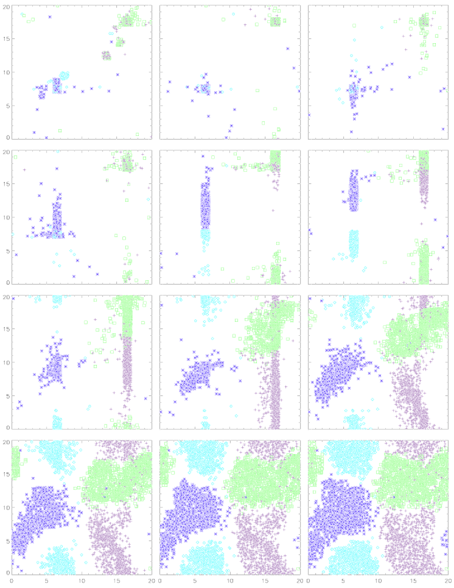
Figure 3: Evolution of a network trained with our synthetic data and with $\alpha(t)=\alpha_{0}=0.01$. Panels show (from left to right, top to bottom), iterations 1, 4, 7, 10, 13, 16, 19, 22, 25, 28, 31, 34. The four classes of synthetic lightcurve (described in Section 3.2.1) are denoted by (i) squares, (ii) crosses, (iii) diamonds and (iv) stars. Note that, for the purposes of visualisation, the positions of all lightcurves have been randomised within their host neurons.

3.2.2 Learning behaviour of the network

Figure 3 shows the evolution of a typical network. In this example the $\alpha$ parameter is held constant at 0.01 throughout. The full run had a resolution of 34 iterations. Figure 3 shows every third iteration and, for purposes of visualisation, the positions of all lightcurves have been randomised within their host neurons.

It can be seen in Fig. 3 that the 5000 lightcurves initially form two tight clusters. This is because the synthetic lightcurves naturally divide into two basic types (single and double peaked) and because the large smoothing kernel does not allow the network to form sufficient structure to resolve the lightcurve sub-types. The lightcurves are tightly clustered because the large smoothing length forces the clusters to strongly repel one another. Weak cross-shaped structures are also apparent, and are a natural consequence of the wrapping of the Gaussian kernel in both dimensions. As the network is evolved, and the kernel size is decreased, the network becomes increasingly free to develop substructure which better represents the the range of shapes of the synthetic lightcurves. Between iterations 13 and 16 one of the initial clusters splits into two (the contact and detached eclipsing binaries), and between iterations 13 and 22 the other initial cluster also gradually splits (the symmetric and skewed Gaussian shapes). By iteration 22 the map well represents the four types of lightcurve. As the kernel size continues to decrease the clusters repel each other less strongly and begin to spread to occupy more of the available neurons. This is because sharper differences in the template lightcurves are now allowed between neighbouring neurons. The increasing size of the clusters allow them to better describe the range of sub-structure within each type of lightcurve, and smooth variations of lightcurve properties are seen across the individual clusters. Finally, as the smoothing kernel decreases below the separation of individual neurons, neighbouring neurons become decoupled and the clusters can make contact. At this point the network has evolved to the point that all of its neurons are representing subtly different lightcurve shapes, and learning is complete.

3.2.3 Monitoring learning performance

The learning behaviour of our maps motivates us to track three measures which allow us to quantify the degree of re-organisation which is taking place at a given time, and the quality of the match between the template lightcurves and the training set members assigned to them.

Figure 4: The average “goodness of fit”, $\bar{S}$. In the leftmost column the learning parameter $\alpha$ is held constant throughout the learning phase. In the central column $\alpha$ falls linearly, and in the rightmost column exponentially. The initial value of $\alpha$ assumes the value 0.9 (top row), 0.5 (second row), 0.1 (third row) and 0.01 (bottom row).

Figure 5: The number of training set members that move from one iteration to the next, $n_{\mathit{move}}$. Panel order is the same as Figure 4.

Figure 6: The average Euclidean distance moved by a training set member in map space from one iteration to the next, $\bar{D}$. Panel order is the same as Figure 4.

The first of these measures ($\bar{S}$) is the value of $S_{ic,min}$ averaged over all members $i$ of the training set. The statistic $S_{ic,min}$ can be regarded as a measure of the goodness-of-fit between a training set member and the template lightcurve of the network neuron $c$ which most closely matches it. By averaging over all members of the training set we can therefore measure how well the template lightcurves of the network as a whole have adjusted to represent the input data. We expect $\bar{S}$ to remain high during early iterations, to show a rapid fall once the network becomes free to represent all the lightcurve sub-types as separate groups, and then to exhibit a slower decline as finer adjustments are made to the template lightcurves.

The second measure ($n_{\mathit{move}}$) is a count of the number of training set members that have changed location in map space from one iteration to the next. We expect maximum movement at times of maximum learning.

The final measure ($\bar{D}$) is the average Euclidean distance moved by a training set member in map space from one iteration to the next. Again, we expect maximum movement at times of maximum learning.

Figures 4, 5 and 6 show the evolution of $\bar{S}$, $n_{\mathit{move}}$ and $\bar{D}$ as networks are trained using the synthetic lightcurves described above. Several training runs were made, differing only in the initial value chosen for $\alpha$, and the functional form with which $\alpha$ evolves. We choose three functional forms for alpha: a constant value $\alpha(t)=\alpha_{0}$, a linear form $\alpha(t)=\alpha_{0}(1-t)$, and an exponential form $\alpha(t)=\alpha_{0}\exp(-\lambda t)$, where the scaling constant $\lambda$ is chosen such that $\alpha=10^{-3}$ in the final iteration.

Taken together these three figures illustrate that the ability of the map to robustly self-organise is not critically dependent on the choice of either $\alpha_{0}$ or the functional form of $\alpha(t)$. In particular Fig. 4 shows that the template lightcurves adjust to faithfully represent the input data in all cases. All panels in Fig. 4 show a monotonic improvement in the fit statistic that begins relatively slowly while $\sigma$ is high, becomes more rapid when $\sigma$ reaches a critical value that allows all types of lightcurve to be represented by their own grouping in the network, and finally slows as the maps approach a steady state at the end of the learning process. The final value of $\bar{S}$  is similar in all cases except in Fig. 4(l). This run refers to an exponential decrease in $\alpha$ from 0.01 to 0.001. It is clear from this panel that $\alpha$ can drop too fast too soon, thereby “freezing in” structure in the network and prematurely ending learning. For this reason we favour a constant $\alpha(t)$ that allows equal learning at all stages of the learning process. We also do not use $\alpha$ values substantially below 0.01 (although lower values may be acceptable as long as the map is given sufficient time to evolve into equilibrium).

Figures 5 and 6 reveal more details of the learning process. Once again, most panels show broadly the same behaviour, with most learning occurring during the middle of the run, and less at the beginning and ends. It is clear, however, that movement of lightcurves within the map is a function of $\alpha$. For $\alpha_{0}\la 0.2$ the evolution of the map appears to be stable, with individual clusters moving and evolving slowly and consistently with iteration. For larger values of $\alpha_{0}$, however, we have noticed that although large-scale structure does indeed form, that the cluster pattern as a whole continues to migrate rapidly through map space (Figure 5a, 5b, 5d & 5e). In a real-world application this mobility and constant restructuring would quite likely prove to be undesirable. For this reason we prefer to choose values of $\alpha_{0}\la 0.2$.

The rapid learning apparent in the middle iterations in Figs. 4, 5 & 6 reveals the presence of a critical value of $\sigma$ which allows the network sufficient freedom to well represent all classes of lightcurve. This critical $\sigma$ is likely to take a different value for different datasets (more classes would require more freedom and a smaller $\sigma_{\rm crit}$) but nevertheless, in a real-world application, one might choose to save computing effort by starting $\sigma_{0}$ at a value closer to $\sigma_{\rm crit}$.

There is evidence of some misclassification in the final trained network in Fig. 3, for example between skewed and non-skewed Gaussian profiles. This is not unexpected as some members of the skewed Gaussian class will exhibit a very small degree of skewness, and are difficult to distinguish from the non-skewed class members even when inspected by eye. Misclassification is difficult to avoid in any situation where there is a smooth trend in variation of light-curve shape between two classes, emphasising that in real-world applications shape-based classification would be used alongside other diagnostic attributes. Nevertheless as a whole the algorithm has performed remarkably well.

3.3 A test with real lightcurves

In order to test the classification abilities of the self-organising map using real data we chose to train it using lightcurves from the ROTSE experiment. The training set consisted of 1206 periodic lightcurves which had been independently pre-classified by other means (Akerlof et al., 2000). The externally derived classifications were not used in training our network, however they did allow us to assess the ability of the algorithm to group and classify class members after training is complete.

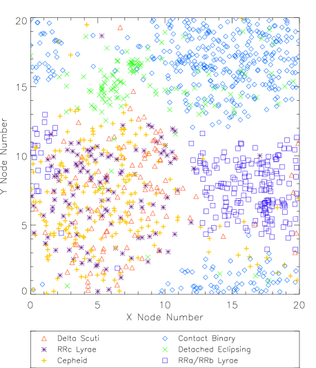
Figure 7: The final structure of a network trained using 1206 pre-classified ROTSE lightcurves.

Figure 7 shows the final state of a network trained using the ROTSE lightcurves. All parameters were set to the same values as the run in Fig. 3, in particular $\alpha$ was held at a value of 0.01 throughout. It can be seen that our algorithm has successfully differentiated the contact binaries, the detached eclipsing binaries, and the type-ab RR Lyrae systems. The remaining three classes in the sample, Cepheids, $\delta$ Scuti and type-c RR Lyrae stars, possess very similar lightcurve profiles (indeed the variability is driven by the same underlying physical process), therefore the network cannot distinguish between the classes on shape alone. In such cases, however, the use of additional information can be used to resolve the ambiguity. In Fig. 8 we show an example of how this additional information can be used. This figure shows the map of Fig. 7 collapsed in one dimension and expanded with the period of the variable star. The $\delta$ Scuti, Cepheid and type-c RR Lyrae variables, which formed an overlapping group in Fig. 7, have been separated in period with clearly defined cut-off boundaries for each type.

Some misidentification of lightcurves is apparent in Fig. 7. We have investigated a number of cases and are confident that our maps have classified the data correctly. The discrepancies seem to be the result of occasional misclassification in the original ROTSE analysis.

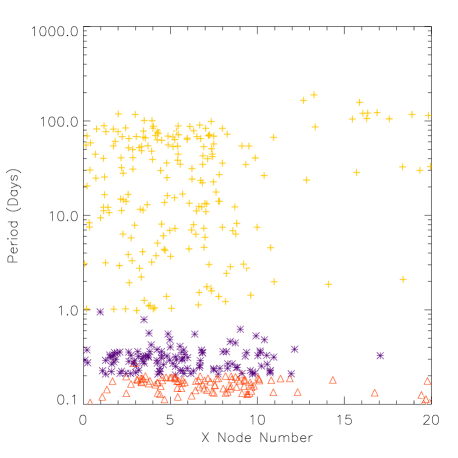
Figure 8: The ROTSE map of Fig. 7 collapsed in one dimension and expanded with the period of the variable star. Here the $\delta$ Scuti, Cepheid and type-c RR Lyrae variables, which formed an overlapping group in Fig. 7, have been separated in period. This illustrates how additional information can be used to resolve ambiguity in our maps, which are based on shape alone.

4 Automated extraction of Clusters

Once training is complete and the map has self organised, it may in some applications be desirable to proceed further to automatically identify “clusters” within the map. Such a cluster extraction step would then allow the automatic assignment of a classification to each member of the input set.

The most obvious approach to cluster extraction is a direct examination of the distribution of training set members in map space. One potential drawback of this approach is that the Kohonen scheme tends to spread the input members fairly uniformly throughout the map space (Fig. 3, see also Kohonen, 1990). This could be a particular problem in the case of small or noisy datasets, such as the ROTSE data (Fig. 7); in such cases the boundaries between clusters could become difficult to identify. Figure 9 shows the number of training set members assigned to each neuron for the ROTSE data set. A small degree of smoothing has been applied to this map to reduce noise due to small-number statistics in the map bins. The clusters and cluster boundaries are readily visible.

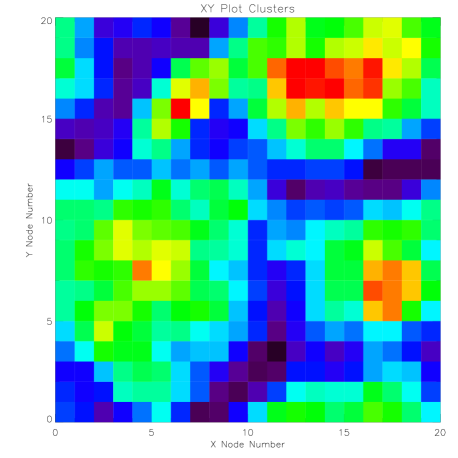
Figure 9: A map of the number of training set members assigned to each neuron for the network trained with the ROTSE data. The raw map has been filtered with a 3x3 top-hat kernel. The colour scale runs from black (low occupancy) to red (high occupancy).

Ultsch & Siemon (1990) outline a different approach to the problem by calculating what they call the U-matrix. In essence the U-matrix attempts to capture the rate of change of shape in the neuron reference vectors across the map space; within clusters adjacent neurons will have reference vectors which are rather similar to each other, whereas at boundaries the differences will be more marked.

The difference between the reference vector of a neuron, $i$, and that of one of its near neighbours, $j$, can be calculated as:

$$L=\sum_{q}{(w_{iq}-w_{jq})^{2}}$$

In a two-dimensional map each neuron will have eight nearest neighbours, so we calculate $L$ for each neighbour in turn and take the average. Figure 10 shows the resulting map calculated from the same trained network as Figure 9. The U-matrix map also readily reveals the clusters and their boundaries, and with noticeably less noise than the number density distribution map.

Both the number density and the U-matrix maps would be suitable for further processing to identify contiguous areas enclosed within the cluster boundaries. It is worth noting however that because the U-matrix is comparing the shape of the templates, rather than number counts in the training set, the resulting map is less susceptible to noise in cases where the training set is of limited size.

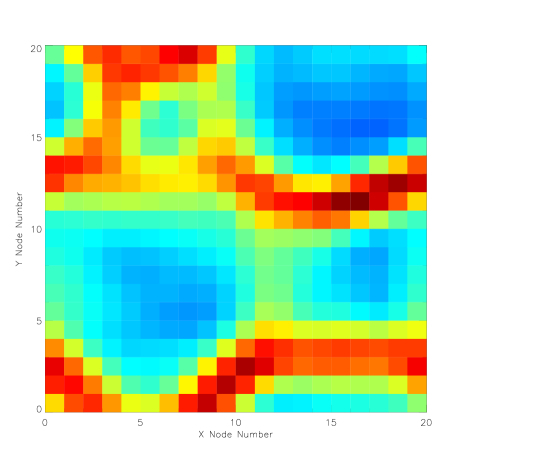
Figure 10: The final iteration of the ROTSE data map (shown in Fig. 7) when processed with the U-Matrix algorithm. The colour scale runs from dark blue (similar reference vectors) to red (dissimilar reference vectors).

5 Conclusions

We have applied the Kohonen self-organising map scheme to the classification of singly periodic astronomical lightcurves. Our algorithm has proved capable of reliably classifying both synthetic and real lightcurves. The investigation has also shown that the ability of the map to robustly self-organise is not strongly dependent on the parameters used to control the learning process.

We conclude that the self-organising map will prove a valuable addition to the data-mining toolset for future large time-domain datasets.

References

- Akerlof et al. (2000) Akerlof C., Amrose S., Balsano R., Bloch J., Casperson D., Fletcher S., Gisler G., Hills J., Kehoe R., Lee B., Marshall S., McKay T., Pawl A., Schaefer J., Szymanski J., Wren J., 2000, AJ, 119, 1901
- Alonso et al. (2003) Alonso R., Belmonte J. A., Brown T., 2003, Astrophys. Space. Sci., 284, 13
- Eyer & Blake (2002) Eyer L., Blake C., 2002, in ASP Conf. Ser. 259: IAU Colloq. 185: Radial and Nonradial Pulsationsn as Probes of Stellar Physics. Automated classification of variable stars for asas data. p. 160
- Fuentes (2001) Fuentes O., 2001, Experimental Astronomy, 12, 21
- Hernandez-Pajares & Floris (1994) Hernandez-Pajares M., Floris J., 1994, MNRAS, 268, 444
- Kane et al. (2003) Kane S. R., Horne K., Street R. A., Pollaco D. L., James D., Tsapras Y., Collier Cameron A., 2003, in ASP Conf. Ser. 294: Scientific Frontiers in Research on Extrasolar Planets Recent Results from the Wide Angle Search for Planets (WASP) Prototype. pp 387–390
- Kohonen (1990) Kohonen T., 1990, Proc. IEEE, 78, 1464
- Mähönen & Hakala (1995) Mähönen P. H., Hakala P. J., 1995, ApJ, 452, L77
- Miller & Coe (1996) Miller A. S., Coe M. J., 1996, MNRAS, 279, 293
- Molinari & Smareglia (1998) Molinari E., Smareglia R., 1998, A&A, 330, 447
- Naim et al. (1997) Naim A., Ratnatunga K. U., Griffiths R. E., 1997, ApJS, 111, 357
- Poincot et al. (1998) Poincot P., Lesteven S., Murtagh F., 1998, A&AS, 130, 183
- Pojmanski (1997) Pojmanski G., 1997, Acta Astron., 47, 467
- Pojmanski (2002) Pojmanski G., 2002, Acta Astron., 52, 397
- Rajaniemi & Mähönen (2002) Rajaniemi H. J., Mähönen P., 2002, ApJ, 566, 202
- Street et al. (2003) Street R. A., Pollaco D. L., Fitzsimmons A., Keenan F. P., Horne K., Kane S., Collier Cameron A., Lister T. A., Haswell C., Norton A. J., Jones B. W., Skillen I., Hodgkin S., Wheatley P., West R., Brett D., 2003, in ASP Conf. Ser. 294: Scientific Frontiers in Research on Extrasolar Planets SuperWASP: Wide Angle Search for Planets. pp 405–408
- Ultsch & Siemon (1990) Ultsch A., Siemon H. P., 1990, in Proc. Int. Neural Networks Conf. Kohonen’s self organising feature maps for exploratory data analysis. Dordrecht: Kluwer, pp 305–308
- Vestrand et al. (2002) Vestrand W. T., Borozdin K. N., Brumby S. P., Casperson D. E., Fenimore E. E., Galassi M. C., McGowan K., Perkins S. J., Priedhorsky W. C., Starr D., White R., Wozniak P., Wren J. A., 2002, in Advanced Global Communications Technologies for Astronomy II. Edited by Kibrick, Robert I. Proceedings of the SPIE, Volume 4845, pp. 126-136 (2002). The RAPTOR experiment: a system for monitoring the optical sky in real time. p. 126
- Wozniak et al. (2004) Wozniak P. R., et al., 2004, ApJ, in press