Entrainment coefficient and effective mass for conduction neutrons in neutron star crust: Macroscopic treatment.

Abstract.

Phenomena such as pulsar frequency glitches are believed to be attributable to differential rotation of a current of “free” superfluid neutrons at densities above the “drip” threshold in the ionic crust of a neutron star. Such relative flow is shown to be locally describable by adaption of a canonical two fluid treatment that emphasizes the role of the momentum covectors constructed by differentiation of action with respect to the currents, with allowance for stratification whereby the ionic number current may be conserved even when the ionic charge number ${\color[rgb]{0.6,0.4,0.0}Z}$ is altered by beta processes. It is demonstrated that the gauge freedom to make different choices of the chemical basis determining which neutrons are counted as “free” does not affect their “superfluid” momentum covector, which must locally have the form of a gradient (though it does affect the “normal” momentum covector characterising the protons and those neutrons that are considered to be “confined” in the nuclei). It is shown how the effect of “entrainment” (whereby the momentum directions deviate from those of the currents) is controlled by the (gauge independent) mobility coefficient ${\color[rgb]{0.4,0,0.2}{\cal K}}$ , estimated in recent microscopical quantum mechanical investigations, which suggest that the corresponding (gauge dependent) “effective mass” ${\color[rgb]{1,0,0}m}_{\star}$ of the free neutrons can become very large in some layers. The relation between this treatment of the crust layers and related work (using different definitions of “effective mass”) intended for the deeper core layers is discussed.

1 Introduction

As a prerequisite for the quantitative analysis of the role of differential rotation in the angular momentum transfer mechanism that is thought [1] to be responsible for phenomena such as pulsar glitches, the purpose of this article is to describe the adaptation to the special circumstances pertaining to the inner crust of a neutron star of the kind of non relativistic two constituent fluid formalism that has already been applied [2, 3] to the global description of the main bulk of the star, in which the basic constituents are relatively moving currents of protons and neutrons, using a treatment of the non-dissipative kind [4, 5] that has recently been developed in a variational formulation [6, 7, 8] that, although non-relativistic, can nevertheless be very conveniently expressed in a fully covariant manner [9, 10]. (A non-dissipative treatment is useful as a good first approximation in view of the superfluidity of the neutrons, but in any case, after the appropriate action function has been obtained in the manner described below, it will be possible to use it as an equation of state in a less idealised model of the kind [11] needed to allow for dissipation and for the relativistic effects [12] that are important at a global level.)

Such a two fluid treatment does not take account of the third independent current, namely that of the electrons, that is of dominant importance for electromagnetic effects, but which makes a relatively negligible contribution to the Newtonian mass transport effects under consideration here. Allowance will however be made here for an important special feature of the crust layers (providing stratification that contributes to stability against convection) namely the clustering of the protons into ions, whose number current can remain conserved even after allowance for possible variation of the ionic charge number ${\color[rgb]{0.6,0.4,0.0}Z}$ due to weak interactions whereby protons are transformed into neutron or vice versa. Another special stabilising feature of the crust that will also need to be allowed for, but that will be left for subsequent work is that of the (relatively small) stress anisotropy that can arise from the elastic solidity [14] of the crust, or from strong magnetic fields [13].

The present article is particularly concerned rather with allowance for the effect of relative “entrainment” [15] between on one hand the effectively free neutrons that will be present above the “neutron drip” density threshold (of the order of $10^{11}$ g/cm³) and that are expected to behave as a superfluid except at very high temperature, and on the other hand the protons, which (together with the ions to which they are confined) will behave as an effectively “normal” fluid in the crust, though they may behave as another superfluid in the deeper layers at densities above the nuclear threshold of the order of $10^{14}$ g/cm³ at which the ions merge.

One of the main goals of this article is to clarify the relationships between different kinds [4, 5] of definition of “effective mass” that have been introduced by various authors as a quantitative measure of the “entrainment” effect, and particularly to provide a discussion of the way such masses depend on the gauge freedom involved in the choice of a chemical basis for the purpose of specifying just which neutrons are considered to be free. In the homogeneous (unclustered) phase above the nuclear density threshold prevailing in the liquid core the neutrons will all be effectively free, while in the outer crust below the “drip” threshold it is clear that none of them will be free, in the “operational” sense of being able to penetrate the potential barriers between nuclei in an astrophysical timescale shorter than the age of the universe. In the inner crust at densities just above this threshold, neutrons in low and intermediate energy states will still be effectively confined, but there will be a clear cut critical energy above which they will be effectively free to travel over ionic separation distances on a microscopically short timescale.

The problem is that, at deeper levels in the crust, such an “operational” discrimination between “confined” and “free” neutron states will no longer be so clear cut, because the ionic wells will get too close for the exponential suppression outside to be fully effective, so that there will be marginally bound states with intermediate penetration timescales that are macroscopically long but cosmologicaly short. This means that there will be some degree of ambiguity that needs to be resolved by a more or less arbitrary choice of a chemical gauge whereby the baryon number ${\color[rgb]{0,0,0}A}\$ of the ionic clusters is prescribed as a function of their (depth dependent) charge number ${\color[rgb]{0.6,0.4,0.0}Z}$ . Fortunately, as will be shown below, the most important quantities in the two fluid formalism at a local (intervortex) level notably the action density $\Lambda$ with its concomitant energy function, and in particular the (irrotational) superfluid neutron momentum, all turn out to be robustly independent of which particular (“operational” or other) gauge criterion is used.

Following this discussion of the different ways of formulating the generic treatment of entrainment in the two fluid formalism, a more particular purpose of this work is to show how quantitative values of the relevant “effective mass” are provided by the corresponding (gauge independent) “mobility coefficient” ${\color[rgb]{0.4,0,0.2}{\cal K}}$ for which quantitative estimates are obtainable from the kind of microscopic analysis described in our immediately preceding work [16]. This analysis is based on a non-relativistic quantum mechanical formalism of the type introduced by Oyamatsu and Yamada [17] in a local frame with respect to which the ionic crust lattice is at rest, so that it gives rise to a static effective potential having a periodic dependence on the cartesian space coordinates $x^{i}$ . The analysis is carried out in terms of single particle wave functions subject to Bloch type boundary conditions (meaning that they deviate from ordinary periodicity by a phase factor of the form $\exp\{{\rm i}{\color[rgb]{0,0.6,0.0}k}_{i}x^{i}\}$ ) of the kind that is commonly used for electrons in ordinary solid state physics, but that has not yet been systematically employed for analogous problems involving neutrons. In a follow up article [18] we have shown how the method can be extended to include the moderate adjustments arising from the effect of BCS type superfluid pairing.

The mobility coefficient ${{\color[rgb]{0.4,0,0.2}{\cal K}}}$ , that is provided by this analysis, has a value which is interpretable as the ratio of the density ${\color[rgb]{0,0.6,0.0}n}$ of “free” (“conduction”) neutrons to their effective mass ${\color[rgb]{1,0,0}m}_{\star}$ . It was suggested by our preliminary results [16] and has been confirmed by more recent work  [19] that this value is likely to be much larger than had been expected. Even when measured with respect to an “operational” gauge as shown in Figure 4 in which the number density ${\color[rgb]{0,0.6,0.0}n}$ of neutrons that are counted as “free” allows only for those that are not bound inside ionic nuclei, the quantity ${\color[rgb]{1,0,0}m}_{\star}$ is likely to become extremely large compared with the ordinary neutron mass ${\color[rgb]{1,0,0}m}$ in the middle layers of the inner crust. It would of course be even larger with respect to the very simple “comprehensive” gauge in which all the neutrons are counted as “free” so that, as shown in Figure 3, the corresponding “effective mass” would in any case diverge as the density decreases to the “neutron drip” value.

The purely Newtonian (i.e. non relativistic) framework within which the work of the present article is carried out should be adequate, on a local scale, as a fairly good approximation in the density regime under consideration. This lower crust regime extends from the “neutron drip” threshold to the transition to a purely fluid (at low temperatures actually superfluid) mixture of neutrons and protons at the base of the crust where the mean density approaches that of ordinary nuclear matter (at a value of the order of about $10^{14}\,{\rm g.cm}^{-3}.$) In a global representation of the neutron star (on scales of the order of a kilometer or more) there will be significant deviations from flat geometry whose quantitative treatment would require the use of General Relativity, but the discussion here will be limited to a local neighbourhood that is sufficiently small (on scales of the order of a centimeter or less) to be treated as approximately homogeneous and geometrically flat. Even on such a purely local scale it would be necessary to use a special relativistic (Minkowski space) description if we were concerned with effects involving the electrons, but the rest mass of the neutrons, to which the present analysis is restricted, is so much higher that a purely Newtonian analysis should be quite adequate in the moderate energy range (up to a few tens of MeV) that is involved. This contrasts with the state of affairs in the fluid core of the neutron star, where estimation of the relevant “entrainment” between (superfluid) neutrons and protons requires a different kind of treatment [20] in which allowance for relativity is important, but where the effect of the entrainment is much more moderate. An implication is that to improve on previous work [21] that ignored the effects both of relativity and of entrainment in the analysis of angular momentum transfer in the crust, the effect of relativity is of secondary importance, and that the first priority is to include the relevant allowance for the effective mass enhancement due to entrainment [22].

2 Generic two-fluid models with stratification

2.1 The canonical master function

In astrophysical contexts for which a non-relativisitic Newtonian mechanical description is adequate it will usually be sufficiently accurate to represent the relevant distribution of mass just in terms of a conserved current of baryons characterised by a single constant mass parameter, ${\color[rgb]{1,0,0}m}$ say, that can be taken to be the standard atomic mass unit or simply the proton mass which is different only by a fraction of a per cent and so is near enough for practical purpose. It is convenient for many purposes to use a 4-dimensional notation scheme [9, 10, 11] in which, for example, the total baryon number density ${\color[rgb]{0,0.6,0.0}n}_{\rm b}$ say, and the corresponding baryon current density components ${\color[rgb]{0,0.6,0.0}n}_{{\rm b}}^{\,i}$ with respect to space coordinates $x^{i}$ $(i=1,2,3)$ are combined to form a 4-current ${\color[rgb]{0,0.6,0.0}n}_{{\rm b}}^{\,\nu}$ $(\nu=0,1,2,3)$ whose time component is given by ${\color[rgb]{0,0.6,0.0}n}_{{\rm b}}^{{}^{{}_{0}}}={\color[rgb]{0,0.6,0.0}n}_{{\rm b}}$ . This means that the total baryon conservation law,

$$\color[rgb]{0,0,0}{\partial{\color[rgb]{0,0.6,0.0}n}_{{\rm b}}/\partial t}+\nabla_{\!i\,}{\color[rgb]{0,0.6,0.0}n}_{{\rm b}}^{\,i}=0\,,$$ (2.1)

will be expressible more concisely as

$$\color[rgb]{0,0,0}\nabla_{\!\nu}{\color[rgb]{0,0.6,0.0}n}_{{\rm b}}^{\,\nu}=0\,.$$ (2.2)

(Throughout this paper, summation over repeated indices is assumed).

Our purpose here is to consider situations involving relative motion between an uncharged contribution ${\color[rgb]{0,0.6,0.0}n}_{{\rm n}}^{\,\nu}$ that will be attributable mainly to neutrons (but perhaps including other neutral hyperons such as the $\Lambda$ in the inner core regions) and an electrically charged contribution ${\color[rgb]{0,0.6,0.0}n}_{{\color[rgb]{0.6,0.4,0.0}\rm p}}^{\,\nu}$ that will similarly be attributable mainly to protons. (It is to be understood that overall electrical charge balance is ensured by a non baryonic current attributable mainly to electrons, whose mass contribution is so small that it can be neglected.) The two independent baryonic contributions combine to give the conserved total baryon current

$$\color[rgb]{0,0,0}{\color[rgb]{0,0.6,0.0}n}_{{\rm b}}^{\,\nu}={\color[rgb]{0,0.6,0.0}n}_{{\rm n}}^{\,\nu}+{\color[rgb]{0,0.6,0.0}n}_{{\color[rgb]{0.6,0.4,0.0}\rm p}}^{\,\nu}\,.$$ (2.3)

In dynamic processes on short timescales the neutron and proton currents may each be considered to be separately conserved, meaning that the 4-divergences $\nabla_{\!\nu}{\color[rgb]{0,0.6,0.0}n}_{{\rm n}}^{\,\nu}$ and $\nabla_{\!\nu}{\color[rgb]{0,0.6,0.0}n}_{{\color[rgb]{0.6,0.4,0.0}\rm p}}^{\,\nu}$ will both vanish individually, but in long term “secular” evolution processes it will be necessary to allow for the possibility of converting neutrons to protons or vice versa by weak interaction processes.

The present discussion will be concerned with cases in which the evolution of the separate contributions ${\color[rgb]{0,0.6,0.0}n}_{{\rm n}}^{\,\nu}$ and ${\color[rgb]{0,0.6,0.0}n}_{{\color[rgb]{0.6,0.4,0.0}\rm p}}^{\,\nu}$ can be described by a multiconstituent fluid model of the kind governed by a master function ${\color[rgb]{1,0,0}\Lambda}_{\rm mat}$ , that acts as the material (meaning non gravitational) part of a Lagrangian in effectively conservative applications [9, 10], but that is also compatible with allowance for potentially relevant dissipative effects [11]. Such a multifluid description does however entail neglect of the extra energy contributions due to possible elastic solid deformations [14], and to frozen in magnetic fields [13], whose inclusion would require a more elaborate treatment. As well as depending on the separate currents ${\color[rgb]{0,0.6,0.0}n}_{{\rm n}}^{\,\nu}$ and ${\color[rgb]{0,0.6,0.0}n}_{{\color[rgb]{0.6,0.4,0.0}\rm p}}^{\,\nu}$ it is useful to allow for the potentially important effect of stratification due to baryonic clustering forming ionic nuclei characterised by a charge number ${\color[rgb]{0.6,0.4,0.0}Z}$ and hence by a number density that is expressible as

$$\color[rgb]{0,0,0}{\color[rgb]{0,0.6,0.0}n}_{{\rm I}}={\color[rgb]{0,0.6,0.0}n}_{{\color[rgb]{0.6,0.4,0.0}\rm p}}/{\color[rgb]{0.6,0.4,0.0}Z}\,,$$ (2.4)

wherever the density is below the saturation density of the order of $10^{14}$ g.cm³. This means that the generic variation of the master function will be given in terms of corresponding partial derivative coefficients by an expression of the form

$$\color[rgb]{0,0,0}\delta{\color[rgb]{1,0,0}\Lambda}_{\rm mat}=-{\color[rgb]{1,0,0}\mu}^{{\rm I}}\,\delta{\color[rgb]{0,0.6,0.0}n}_{{\rm I}}+{\color[rgb]{1,0,0}\mu}^{{\rm n}}_{\,\nu}\,\delta{\color[rgb]{0,0.6,0.0}n}_{{\rm n}}^{\,\nu}+{\color[rgb]{1,0,0}\mu}^{{\color[rgb]{0.6,0.4,0.0}\rm p}}_{\,\nu}\,\delta{\color[rgb]{0,0.6,0.0}n}_{{\color[rgb]{0.6,0.4,0.0}\rm p}}^{\,\nu}\,,$$ (2.5)

or equivalently in the less compact form of a traditional 3+1 space time decomposition by an expression of the form

$$\color[rgb]{0,0,0}\delta{\color[rgb]{1,0,0}\Lambda}_{\rm mat}=-{\color[rgb]{1,0,0}\mu}^{{\rm I}}\,\delta{\color[rgb]{0,0.6,0.0}n}_{{\rm I}}-{\color[rgb]{1,0,0}\mu}^{{\rm n}}\,\delta{\color[rgb]{0,0.6,0.0}n}_{{\rm n}}-{\color[rgb]{1,0,0}\mu}^{{\color[rgb]{0.6,0.4,0.0}\rm p}}\,\delta{\color[rgb]{0,0.6,0.0}n}_{{\color[rgb]{0.6,0.4,0.0}\rm p}}+{\color[rgb]{1,0,0}\mu}^{{\rm n}}_{\,i}\,\delta{\color[rgb]{0,0.6,0.0}n}_{{\rm n}}^{\,i}+{\color[rgb]{1,0,0}\mu}^{{\color[rgb]{0.6,0.4,0.0}\rm p}}_{\,i}\,\delta{\color[rgb]{0,0.6,0.0}n}_{{\color[rgb]{0.6,0.4,0.0}\rm p}}^{\,i}\,,$$ (2.6)

in which ${\color[rgb]{1,0,0}\mu}^{{\rm n}}_{i}$ and ${\color[rgb]{1,0,0}\mu}^{{\color[rgb]{0.6,0.4,0.0}\rm p}}_{i}$ will be respectively interpretable as the mean momentum per particle of the neutrons and of the protons, while the quantities

$$\color[rgb]{0,0,0}{\color[rgb]{1,0,0}\mu}^{{\rm n}}=-{\color[rgb]{1,0,0}\mu}^{{\rm n}}_{\,{}_{0}}\,,\hskip 28.45274pt{\color[rgb]{1,0,0}\mu}^{{\rm n}}=-{\color[rgb]{1,0,0}\mu}^{{\rm n}}_{\,{}_{0}}\,,$$ (2.7)

will be interpretable as the corresponding neutronic and protonic chemical potentials, while the coefficient ${\color[rgb]{1,0,0}\mu}^{{\rm I}}$ is an ionic cluster potential, whose gradient, if any, represents the effect of stratification. This potential can be used to construct a corresponding 4-momentum covector that is given in terms of the gradient of the Newtonian time coordinate $x^{{}_{0}}=t$ by the formula

$$\color[rgb]{0,0,0}{\color[rgb]{1,0,0}\mu}^{{\rm I}}_{\,\nu}=-{\color[rgb]{1,0,0}\mu}^{{\rm I}}\,t_{\nu}\,,\hskip 28.45274ptt_{\nu}=\nabla_{\!\nu}\,t=\delta^{{}_{0}}_{\,\nu}\,,$$ (2.8)

which means that it has vanishing space components, ${\color[rgb]{1,0,0}\mu}^{{\rm I}}_{\,i}=0,$ as an expression of the fact that (in the Newtonian limit) the clustering contributes only to energy but not to mass.

The models we are considering are intended for application to neutron star matter after it has cooled down sufficiently for its dynamics to be hardly affected by thermal effects, which are not included. These models are to be interpreted as being governed by dynamical equations that are formally identical to those of the heat convecting thermal model presented in the appendix of the work [11] referred to above, with the ionic cluster potential ${\color[rgb]{1,0,0}\mu}^{{\rm I}}$ taking the place of the temperature ${\color[rgb]{1,0,0}\Theta}\ ,$ and with the ionic number density ${\color[rgb]{0,0.6,0.0}n}_{{\rm I}}$ taking the place of the entropy density ${\color[rgb]{0,0.6,0.0}s}$ , so that the entropy current 4-vector ${\color[rgb]{0,0.6,0.0}s}^{\mu}$ is to be replaced here by the ionic number current 4-vector ${\color[rgb]{0,0.6,0.0}n}_{{\rm I}}^{\,\nu}$ as given in terms of the flow 4-vector ${\color[rgb]{0.4,0,0.2}u}_{\rm c}^{\,\nu}$ of the crust by

$$\color[rgb]{0,0,0}{\color[rgb]{0,0.6,0.0}n}_{{\rm I}}^{\,\nu}={\color[rgb]{0,0.6,0.0}n}_{{\rm I}}\,{\color[rgb]{0.4,0,0.2}u}_{\rm c}^{\,\nu}\,,\hskip 28.45274pt{\color[rgb]{0.4,0,0.2}u}_{\rm c}^{\,\nu}={\color[rgb]{0,0.6,0.0}n}_{{\color[rgb]{0.6,0.4,0.0}\rm p}}^{\,\nu}/{\color[rgb]{0,0.6,0.0}n}_{{\color[rgb]{0.6,0.4,0.0}\rm p}}\,\,.$$ (2.9)

In terms of the generalised pressure function

$$\color[rgb]{0,0,0}{\color[rgb]{1,0,0}\Psi}={\color[rgb]{1,0,0}\Lambda}_{\rm mat}+{\color[rgb]{0,0.6,0.0}n}_{{\rm I}}\,{\color[rgb]{1,0,0}\mu}^{{\rm I}}-{\color[rgb]{0,0.6,0.0}n}_{{\color[rgb]{0.6,0.4,0.0}\rm p}}^{\,\nu}{\color[rgb]{1,0,0}\mu}^{{\color[rgb]{0.6,0.4,0.0}\rm p}}_{\,\nu}-{\color[rgb]{0,0.6,0.0}n}_{{\rm n}}^{\,\nu}{\color[rgb]{1,0,0}\mu}^{{\rm n}}_{\,\nu}\,,$$ (2.10)

and the Newtonian gravitational potential $\phi$ the corresponding material energy momentum 4-tensor [10] will therefore be given by

$$\color[rgb]{0,0,0}{\color[rgb]{1,0,0}T}^{\mu}_{\ \,\nu}={\color[rgb]{0,0.6,0.0}n}_{{\rm I}}^{\,\mu}{\color[rgb]{1,0,0}\mu}^{{\rm I}}_{\,\nu}+{\color[rgb]{0,0.6,0.0}n}_{{\color[rgb]{0.6,0.4,0.0}\rm p}}^{\,\mu}{\color[rgb]{1,0,0}\mu}^{{\color[rgb]{0.6,0.4,0.0}\rm p}}_{\,\nu}+{\color[rgb]{0,0.6,0.0}n}_{{\rm n}}^{\,\mu}{\color[rgb]{1,0,0}\mu}^{{\rm n}}_{\,\nu}+{\color[rgb]{1,0,0}\Psi}\delta^{\mu}_{\,\nu}-\phi\,{\color[rgb]{1,0,0}m}{\color[rgb]{0,0.6,0.0}n}_{{\rm b}}^{\,\mu}t_{\nu}\,.$$ (2.11)

This means that, if the only external force is gravitational, the total force balance equation will then be expressible as

$$\color[rgb]{0,0,0}\nabla_{\!\mu}{\color[rgb]{1,0,0}T}^{\mu}_{\ \,\nu}=-{\color[rgb]{1,0,0}m}{\color[rgb]{0,0.6,0.0}n}_{\rm b}\nabla_{\!\nu}\phi\,,$$ (2.12)

while the condition of conservation of entropy in the conservative case is to be replaced here by the ionic cluster conservation condition

$$\color[rgb]{0,0,0}\nabla_{\!\nu}{\color[rgb]{0,0.6,0.0}n}_{{\rm I}}^{\,\nu}=0\,,$$ (2.13)

which can be expected to be valid, not just in short timescale dynamic processes in which there would be separate conservation of the neutrons

$$\color[rgb]{0,0,0}\nabla_{\!\nu}{\color[rgb]{0,0.6,0.0}n}_{{\rm n}}^{\,\nu}=0$$ (2.14)

(and hence also, according to (2.2), of the protons) but even in processes having the much longer timescales needed for weak interactions to adjust the relative numbers of protons and neutrons so as to achieve the condition of “beta equilibrium”, namely vanishing of the affinity

$$\color[rgb]{0,0,0}{\color[rgb]{0.4,0,0.2}{\cal A}}=({\color[rgb]{1,0,0}\mu}^{{\rm n}}_{\nu}-{\color[rgb]{1,0,0}\mu}^{{\color[rgb]{0.6,0.4,0.0}\rm p}}_{\nu}){\color[rgb]{0.4,0,0.2}u}_{\rm c}^{\,\nu}\,,$$ (2.15)

as specified with respect to the “normal” rest frame specified by ${\color[rgb]{0.4,0,0.2}u}_{\rm c}^{\,\nu}$ , which is that of the protons (and therefore also of the ions) as opposed to that of the neutrons, whose superfluidity at low temperatures allows them to retain a relative motion (at densities above the neutron drip threshold) even in a state of exact non dissipative equilibrium. On timescales even longer than needed for the beta equilibrium condition,

$$\color[rgb]{0,0,0}{\color[rgb]{0.4,0,0.2}{\cal A}}=0\,,$$ (2.16)

it is ultimately to be expected that barrier tunnelling processes involving nuclear fission and recombination would lead to violation of (2.13) in such a way as to efface the stratification by allowing the ionic cluster potential ${\color[rgb]{1,0,0}\mu}^{{\rm I}}$ to tend towards zero, but in practice the stratification will commonly survive long enough to have important stabilising consequences, particularly in the outer layers of the neutron star.

To provide a complete system of evolution equations for the dynamic variables ${\color[rgb]{0,0.6,0.0}n}_{\rm I},$ ${\color[rgb]{0,0.6,0.0}n}_{\rm n}^{\,\nu},$ and ${\color[rgb]{0,0.6,0.0}n}_{\color[rgb]{0.6,0.4,0.0}\rm p}^{\,\nu},$ the system consisting of (2.12) and (2.13), together with one of the alternative possibilities (2.14) or (2.16), does not suffice, but must be supplemented by a further condition which can simply be taken to be the mesoscopic neutron superfluidity condition to the effect that the total neutron momentum covector,

$$\color[rgb]{0,0,0}{\color[rgb]{1,0,0}\pi}^{{\rm n}}_{\,\nu}={\color[rgb]{1,0,0}\mu}^{\rm n}_{\,\nu}-\phi\,{\color[rgb]{1,0,0}m}t_{\nu}\,,$$ (2.17)

should be proportional to a phase gradient, taking the form

$$\color[rgb]{0,0,0}{\color[rgb]{1,0,0}\pi}^{{\rm n}}_{\,\nu}={\color[rgb]{1,0,0}\hbar}\nabla_{\!\nu\,}\varphi^{\rm n}\,,$$ (2.18)

in which the phase variable $\varphi^{\rm n}$ has period $\pi$ (not $2\pi$ ) due to the fermionic half integer spin of the neutrons [18]. (This corresponds to a period having the usual value $2\pi$ for the corresponding phase $\varphi=2\varphi^{\rm n}$ for Cooper pairs with momentum covector $2{\color[rgb]{1,0,0}\pi}^{{\rm n}}_{\,\nu}$ .)

2.2 Chemical invariance of superfluid momentum

In order to obtain a formulation that is consistent with traditional usage in the low density regime with density less than the order of $10^{11}$ g.cm³ for which the neutrons will also be effectively confined within the nuclei, it is useful to introduce a dependent variable, ${\color[rgb]{0,0,0}A}_{\rm c}$ , that is to be interpreted as the total number of effectively “confined” baryons per nucleus, and that specifies a corresponding “confined” baryon number current ${\color[rgb]{0,0.6,0.0}n}_{{\rm c}}^{\,\nu}$ , which will be given by

$$\color[rgb]{0,0,0}{\color[rgb]{0,0.6,0.0}n}_{{\rm c}}^{\,\nu}={\color[rgb]{0,0,0}A}_{\rm c}{\color[rgb]{0,0.6,0.0}n}_{{\rm I}}^{\,\nu}\,.$$ (2.19)

The“confined” baryon number ${\color[rgb]{0,0,0}A}_{\rm c}={\color[rgb]{0,0.6,0.0}n}_{\rm c}/{\color[rgb]{0,0.6,0.0}n}_{\rm I}$ will evidently lie somewhere in the range ${\color[rgb]{0.6,0.4,0.0}Z}\leq{\color[rgb]{0,0,0}A}_{\rm c}\leq{\color[rgb]{0,0,0}A}_{\rm b}$ where ${\color[rgb]{0,0,0}A}_{\rm b}={\color[rgb]{0,0.6,0.0}n}_{\rm b}/{\color[rgb]{0,0.6,0.0}n}_{\rm I}$ is the total baryon number per nucleus, which will of course be the same as ${\color[rgb]{0,0,0}A}_{\rm c}$ at densities below the “neutron drip” threshold. As a corollary there will also be a corresponding “free” neutron current given by

$$\color[rgb]{0,0,0}{\color[rgb]{0,0.6,0.0}n}_{{\rm f}}^{\,\nu}={\color[rgb]{0,0.6,0.0}n}_{{\rm b}}^{\,\nu}-{\color[rgb]{0,0.6,0.0}n}_{{\rm c}}^{\,\nu}\,,$$ (2.20)

which will be non vanishing at densities above the “neutron drip” threshold. In the deeper layers of the ionic “crust” region where the clusters are near to stage of merging they may become highly deformed to “spaghetti” or even “lasagna” shaped configurations [23, 24] for which (as remarked above in the introduction) the meaning of the absolute numbers ${\color[rgb]{0.6,0.4,0.0}Z}$ and ${\color[rgb]{0,0,0}A}$ may become rather hazy, but this need not prevent the ratio

$$\color[rgb]{0,0,0}{\color[rgb]{0,0,0}a}_{\rm c}={\color[rgb]{0,0,0}A}_{\rm c}/{\color[rgb]{0.6,0.4,0.0}Z}={\color[rgb]{0,0.6,0.0}n}_{{\rm c}}/{\color[rgb]{0,0.6,0.0}n}_{{\color[rgb]{0.6,0.4,0.0}\rm p}}$$ (2.21)

of the “confined” baryon number density to the charged baryon number density from remaining definable according to some ansatz that might reasonably be required to specify ${\color[rgb]{0,0,0}a}_{\rm c}$ as a weakly dependent function of ${\color[rgb]{0.6,0.4,0.0}Z}$ in such a way that beyond the transition to an unclustered homogeneous phase above ordinary nuclear matter density, the corresponding “free” neutron current ${\color[rgb]{0,0.6,0.0}n}_{{\rm f}}^{\,\nu}$ will simply become the same as the entire neutron current ${\color[rgb]{0,0.6,0.0}n}_{{\rm n}}^{\,\nu}$ , while at lower densities it would be determined by the equation of state for “cold catalysed” matter whereby all relevant scalars including ${\color[rgb]{0.6,0.4,0.0}Z}$ and ${\color[rgb]{0,0,0}A}_{\rm c}$ are given (in such a way as to minimise the energy density) as functions of ${\color[rgb]{0,0.6,0.0}n}_{\rm b}$ .

However that may be, subject to the specification of any reasonable (realistic or idealised) equation of state for ${\color[rgb]{0,0,0}A}_{\rm c}$ as a function just of ${\color[rgb]{0.6,0.4,0.0}Z}$ so that the variation of the ratio ${\color[rgb]{0,0,0}a}_{\rm c}\{{\color[rgb]{0.6,0.4,0.0}Z}\}$ will be given in terms of its derivative ${\color[rgb]{0,0,0}a}_{\rm c}^{\prime}={\rm d}{\color[rgb]{0,0,0}a}_{\rm c}/{\rm d}{\color[rgb]{0.6,0.4,0.0}Z}$ by an expression of the form

$$\color[rgb]{0,0,0}\delta{\color[rgb]{0,0,0}a}_{\rm c}={\color[rgb]{0.6,0.4,0.0}Z}{\color[rgb]{0,0,0}a}_{\rm c}^{\prime}\left(\frac{\delta{\color[rgb]{0,0.6,0.0}n}_{\color[rgb]{0.6,0.4,0.0}\rm p}}{{\color[rgb]{0,0.6,0.0}n}_{\color[rgb]{0.6,0.4,0.0}\rm p}}-\frac{\delta{\color[rgb]{0,0.6,0.0}n}_{\rm I}}{{\color[rgb]{0,0.6,0.0}n}_{\rm I}}\right)\,,$$ (2.22)

it will be possible, and for some purposes convenient, to make a corresponding chemical basis transformation whereby the new (empirically defined) current variables ${\color[rgb]{0,0.6,0.0}n}_{{\rm f}}^{\,\nu}$ and ${\color[rgb]{0,0.6,0.0}n}_{{\rm c}}^{\,\nu}$ are used in place of the original (more physically fundamental) current variables ${\color[rgb]{0,0.6,0.0}n}_{{\rm n}}^{\,\nu}$ and ${\color[rgb]{0,0.6,0.0}n}_{{\color[rgb]{0.6,0.4,0.0}\rm p}}^{\,\nu}$ as the independent variables of the system. In terms of the new chemical basis, as specified by the homogeneous linear transformation

$$\color[rgb]{0,0,0}{\color[rgb]{0,0.6,0.0}n}_{{\rm f}}^{\,\nu}={\color[rgb]{0,0.6,0.0}n}_{{\rm n}}^{\,\nu}+(1-{\color[rgb]{0,0,0}a}_{\rm c}){\color[rgb]{0,0.6,0.0}n}_{{\color[rgb]{0.6,0.4,0.0}\rm p}}^{\,\nu}\,,\hskip 28.45274pt{\color[rgb]{0,0.6,0.0}n}_{{\rm c}}^{\,\nu}={\color[rgb]{0,0,0}a}_{\rm c}{\color[rgb]{0,0.6,0.0}n}_{{\color[rgb]{0.6,0.4,0.0}\rm p}}^{\,\nu}\,,$$ (2.23)

the generic variation (2.5) of the master function and the corresponding energy momentum tensor (2.11) will be expressible in the exactly analogous forms

$$\color[rgb]{0,0,0}\delta{\color[rgb]{1,0,0}\Lambda}_{\rm mat}=-\tilde{\color[rgb]{1,0,0}\mu}^{{\rm I}}\,\delta{\color[rgb]{0,0.6,0.0}n}_{{\rm I}}+{\color[rgb]{1,0,0}\mu}^{{\rm f}}_{\nu}\,\delta{\color[rgb]{0,0.6,0.0}n}_{{\rm f}}^{\,\nu}+{\color[rgb]{1,0,0}\mu}^{{\rm c}}_{\nu}\,\delta{\color[rgb]{0,0.6,0.0}n}_{{\rm c}}^{\,\nu}\,,$$ (2.24)

and

$$\color[rgb]{0,0,0}{\color[rgb]{1,0,0}T}^{\mu}_{\ \,\nu}={\color[rgb]{0,0.6,0.0}n}_{{\rm I}}^{\,\mu}\tilde{\color[rgb]{1,0,0}\mu}^{{\rm I}}_{\,\nu}+{\color[rgb]{0,0.6,0.0}n}_{{\rm c}}^{\,\mu}{\color[rgb]{1,0,0}\mu}^{{\rm c}}_{\,\nu}+{\color[rgb]{0,0.6,0.0}n}_{{\rm f}}^{\,\mu}{\color[rgb]{1,0,0}\mu}^{{\rm f}}_{\,\nu}+{\color[rgb]{1,0,0}\Psi}\delta^{\mu}_{\,\nu}-\phi\,{\color[rgb]{1,0,0}m}{\color[rgb]{0,0.6,0.0}n}_{{\rm b}}^{\,\mu}t_{\nu}\,,$$ (2.25)

with

$$\color[rgb]{0,0,0}{\color[rgb]{1,0,0}\Psi}={\color[rgb]{1,0,0}\Lambda}_{\rm mat}+{\color[rgb]{0,0.6,0.0}n}_{{\rm I}}\,\tilde{\color[rgb]{1,0,0}\mu}^{{\rm I}}-{\color[rgb]{0,0.6,0.0}n}_{{\rm c}}^{\,\nu}{\color[rgb]{1,0,0}\mu}^{{\rm c}}_{\,\nu}-{\color[rgb]{0,0.6,0.0}n}_{{\rm f}}^{\,\nu}{\color[rgb]{1,0,0}\mu}^{{\rm f}}_{\,\nu}\,,$$ (2.26)

in which the adjusted ionic cluster potential $\tilde{\color[rgb]{1,0,0}\mu}^{{\rm I}}$ and the correspondingly adjusted analogue

$$\color[rgb]{0,0,0}\tilde{\color[rgb]{0.4,0,0.2}{\cal A}}=({\color[rgb]{1,0,0}\mu}^{{\rm f}}_{\nu}-{\color[rgb]{1,0,0}\mu}^{{\rm c}}_{\nu}){\color[rgb]{0.4,0,0.2}u}_{\rm c}^{\,\nu}\,,$$ (2.27)

of the affinity (2.15) will be related to their untransformed analogues by

$$\color[rgb]{0,0,0}{\color[rgb]{0.4,0,0.2}{\cal A}}=\tilde{\color[rgb]{0.4,0,0.2}{\cal A}}({\color[rgb]{0,0,0}a}_{\rm c}+{\color[rgb]{0.6,0.4,0.0}Z}{\color[rgb]{0,0,0}a}_{\rm c}^{\prime})$$ (2.28)

and

$$\color[rgb]{0,0,0}{\color[rgb]{1,0,0}\mu}^{{\rm I}}=\tilde{\color[rgb]{1,0,0}\mu}^{{\rm I}}-{\color[rgb]{0.6,0.4,0.0}Z}^{2}\tilde{\color[rgb]{0.4,0,0.2}{\cal A}}\,{\color[rgb]{0,0,0}a}_{\rm c}^{\prime}\,,$$ (2.29)

while the new “free” and “confined” baryon momentum 4 covectors ${\color[rgb]{1,0,0}\mu}^{{\rm f}}_{\nu}$ and ${\color[rgb]{1,0,0}\mu}^{{\rm c}}_{\nu}$ will be given in terms of their untransformed analogues ${\color[rgb]{1,0,0}\mu}^{{\rm I}},$ ${\color[rgb]{1,0,0}\mu}^{{\rm f}}_{\nu},$ ${\color[rgb]{1,0,0}\mu}^{{\rm c}}_{\nu},$ by the relations

$$\color[rgb]{0,0,0}{\color[rgb]{1,0,0}\mu}^{{\color[rgb]{0.6,0.4,0.0}\rm p}}_{\,\nu}={\color[rgb]{1,0,0}\mu}^{{\rm c}}_{\,\nu}+(1-{\color[rgb]{0,0,0}a}_{\rm c})({\color[rgb]{1,0,0}\mu}^{{\rm f}}_{\,\nu}-{\color[rgb]{1,0,0}\mu}^{{\rm c}}_{\,\nu})-{\color[rgb]{0.6,0.4,0.0}Z}\tilde{\color[rgb]{0.4,0,0.2}{\cal A}}\,{\color[rgb]{0,0,0}a}_{\rm c}^{\prime}t_{\nu}\,$$ (2.30)

and

$$\color[rgb]{0,0,0}{\color[rgb]{1,0,0}\mu}^{{\rm n}}_{\,\nu}={\color[rgb]{1,0,0}\mu}^{{\rm f}}_{\,\nu}\,.$$ (2.31)

This last result is important: it tells us that whereas the momentum covector ${\color[rgb]{1,0,0}\mu}^{{\rm c}}_{\,\nu}$ associated with the “confined” part has a rather complicated dependence on the chemical gauge specified by the choice of the functional dependence of ${\color[rgb]{0,0,0}a}_{\rm c}$ on ${\color[rgb]{0.6,0.4,0.0}Z},$ on the other hand the momentum covector ${\color[rgb]{1,0,0}\mu}^{{\rm f}}_{\,\nu}$ associated with the “free” neutron current is invariant with respect to the change of gauge. The correponding total

$$\color[rgb]{0,0,0}{\color[rgb]{1,0,0}\pi}^{{\rm f}}_{\,\nu}={\color[rgb]{1,0,0}\mu}^{\rm f}_{\,\nu}-\phi\,{\color[rgb]{1,0,0}m}t_{\mu}\,,$$ (2.32)

is just the same as its analogue (2.17) in the original formulation, so that the superfluidity condition (2.18) will be expressible in terms of the the same phase variable $\varphi$ in exactly the same way as before, meaning that it will be given simply by

$$\color[rgb]{0,0,0}{\color[rgb]{1,0,0}\pi}^{{\rm f}}_{\,\nu}={\color[rgb]{1,0,0}\hbar}\nabla_{\!\nu\,}\varphi\,.$$ (2.33)

The upshot of this is that if the set of dynamical equations is completed by the beta equilibrium condition (2.16), which according to (2.28) will be expressible in the language of the new formulation simply by

$$\color[rgb]{0,0,0}\tilde{\color[rgb]{0.4,0,0.2}{\cal A}}=0\,,$$ (2.34)

then the entire system will be chemically covariant in the sense of having the same form regardless of the choice of the gauge function ${\color[rgb]{0,0,0}a}_{\rm c}\{{\color[rgb]{0.6,0.4,0.0}Z}\}$ in the chemical basis transformation (2.23).

On the other hand if (as will be appropriate for cases involving relatively short dynamical timescales) the beta equilibrium condition (2.16) is replaced by the separate neutron current conservation condition (2.14) then the complete system will be chemically covariant only with respect to transformations in which ${\color[rgb]{0,0,0}a}_{\rm c}$ is simply taken to be constant, as for example in what we shall refer to as the “comprehensive gauge”, which is given simply by ${\color[rgb]{0,0,0}a}_{\rm c}=1$ so that absolutely all of the neutrons are classified as “free”, while a less trivial example is that of what may be described as the “paired gauge”, which is given by ${\color[rgb]{0,0,0}a}_{\rm c}=2$ , and which is interpretable as meaning that the only neutrons classified as “confined” are those in the tightly bound states that are directly paired with corresponding proton states in the nuclei. However, if we wish to use ${\color[rgb]{0,0,0}a}_{\rm c}$ to provide a more realisticlly “operational” estimate of the total baryon to proton number ratio in the nuclei, it will need to be given a non vanishing derivative ${\color[rgb]{0,0,0}a}_{\rm c}^{\prime},$ and in that case the corresponding formulation of the separate conservation condition (2.14)   will have the patently gauge dependent form

$$\color[rgb]{0,0,0}\nabla_{\!\nu\,}{\color[rgb]{0,0.6,0.0}n}_{\rm f}^{\,\nu}=-{\color[rgb]{0,0,0}a}_{\rm c}^{\prime}{\color[rgb]{0,0.6,0.0}n}_{\rm c}^{\,\nu}\nabla_{\!\nu\,}{\color[rgb]{0.6,0.4,0.0}Z}\,.$$ (2.35)

2.3 Local energy function

In order to obtain information about the equation of state giving the functional dependence of the material action density ${\color[rgb]{1,0,0}\Lambda}_{\rm mat}$ on the relevant independent variables by comparison with the results of a microphysical analysis, it is convenient to work with the corresponding energy function. The complete energy momentum tensor (2.25)   comes from a complete action density ${\color[rgb]{1,0,0}\Lambda}={\color[rgb]{1,0,0}\Lambda}_{\rm mat}+{\color[rgb]{1,0,0}\Lambda}_{\rm pot}$ in which, as discussed in the previously cited work [10], the gravitational potential energy contribution is given simply by ${\color[rgb]{1,0,0}\Lambda}_{\rm pot}=-{\color[rgb]{1,0,0}\rho}\phi,$ with ${\color[rgb]{1,0,0}\rho}={\color[rgb]{1,0,0}m}{\color[rgb]{0,0.6,0.0}n}_{\rm b}$ so the corresponding energy ${\color[rgb]{1,0,0}U}=-{\color[rgb]{1,0,0}T}^{{}_{0}}_{\ {}_{0}}$ will have the form of a sum ${\color[rgb]{1,0,0}U}={\color[rgb]{1,0,0}U}_{\rm mat}+{\color[rgb]{1,0,0}U}_{\rm pot}$ involving a gravitational contribution ${\color[rgb]{1,0,0}U}_{\rm pot}=-{\color[rgb]{1,0,0}\Lambda}_{\rm pot}$ that must be subtracted off to leave the purely material part ${\color[rgb]{1,0,0}U}_{\rm mat}$ corresponding just to ${\color[rgb]{1,0,0}\Lambda}_{\rm mat}$ . It can thus be seen that this material energy density will be given (for an arbitrary choice of the chemical gauge function ${\color[rgb]{0,0,0}a}_{\rm c}\{{\color[rgb]{0.6,0.4,0.0}Z}\}$ ) by

$$\color[rgb]{0,0,0}{\color[rgb]{1,0,0}U}_{\rm mat}=\tilde{\color[rgb]{1,0,0}\mu}^{{\rm I}}\,{\color[rgb]{0,0.6,0.0}n}_{\rm I}-{\color[rgb]{1,0,0}\mu}^{{\rm f}}_{{}_{0}}\,{\color[rgb]{0,0.6,0.0}n}_{{\rm f}}-{\color[rgb]{1,0,0}\mu}^{{\rm c}}_{{}_{0}}\,{\color[rgb]{0,0.6,0.0}n}_{{\rm c}}-{\color[rgb]{1,0,0}\Psi}\,,$$ (2.36)

which, by (2.26)   , is evidently equivalent to taking

$$\color[rgb]{0,0,0}{\color[rgb]{1,0,0}U}_{\rm mat}={\color[rgb]{1,0,0}\mu}^{{\rm f}}_{i}\,{\color[rgb]{0,0.6,0.0}n}_{{\rm f}}^{\,i}+{\color[rgb]{1,0,0}\mu}^{{\rm c}}_{i}\,{\color[rgb]{0,0.6,0.0}n}_{{\rm c}}^{\,i}-{\color[rgb]{1,0,0}\Lambda}_{\rm mat}\,.$$ (2.37)

So long as the relevant velocities are sufficiently small, it will be possible to decompose the material Lagrangian and energy density in the form

$$\color[rgb]{0,0,0}{\color[rgb]{1,0,0}\Lambda}_{\rm mat}={\color[rgb]{1,0,0}\Lambda}_{\rm ins}+{\color[rgb]{1,0,0}\Lambda}_{\rm dyn}\,,$$ (2.38)

and

$$\color[rgb]{0,0,0}{\color[rgb]{1,0,0}U}_{\rm mat}={\color[rgb]{1,0,0}U}_{\rm ins}+{\color[rgb]{1,0,0}U}_{\rm dyn}\,,$$ (2.39)

in terms of a static internal energy contribution

$$\color[rgb]{0,0,0}{\color[rgb]{1,0,0}U}_{\rm ins}=-{\color[rgb]{1,0,0}\Lambda}_{\rm ins}\,,$$ (2.40)

that will depend only on the relevant ionic and (free and confined) baryon number densities namely ${\color[rgb]{0,0.6,0.0}n}_{{\rm I}},$ ${\color[rgb]{0,0.6,0.0}n}_{{\rm f}},$ ${\color[rgb]{0,0.6,0.0}n}_{{\rm c}}$ , together with a dynamic contribution for which the velocity dependence is homogeneously quadratic so that as for the purely kinetic part [10] the corresponding energy contribution will be the same as the Lagrangian contribution from which it is derived, having the form

$$\color[rgb]{0,0,0}{\color[rgb]{1,0,0}\Lambda}_{\rm dyn}={\color[rgb]{1,0,0}U}_{\rm dyn}=\frac{{}_{1}}{{}^{2}}({\color[rgb]{1,0,0}\mu}^{{\rm f}}_{i}\,{\color[rgb]{0,0.6,0.0}n}_{{\rm f}}^{\,i}+{\color[rgb]{1,0,0}\mu}^{{\rm c}}_{i}\,{\color[rgb]{0,0.6,0.0}n}_{{\rm c}}^{\,i})\,.$$ (2.41)

This means that it will be given as a function of the current components ${\color[rgb]{0,0.6,0.0}n}_{{\rm f}}^{\,i}$ and ${\color[rgb]{0,0.6,0.0}n}_{{\rm c}}^{\,i}\,$ by an expression of the form

$$\color[rgb]{0,0,0}{\color[rgb]{1,0,0}\Lambda}_{\rm dyn}=\frac{{}_{1}}{{}^{2}}\gamma_{ij}\big{(}{{\color[rgb]{0.4,0,0.2}{\cal K}}}^{\rm ff}\,{\color[rgb]{0,0.6,0.0}n}_{{\rm f}}^{\,i}\,{\color[rgb]{0,0.6,0.0}n}_{{\rm f}}^{\,j}+2{{\color[rgb]{0.4,0,0.2}{\cal K}}}^{{\rm fc}}\,{\color[rgb]{0,0.6,0.0}n}_{{\rm f}}^{\,i}\,{\color[rgb]{0,0.6,0.0}n}_{{\rm c}}^{\,j}+{{\color[rgb]{0.4,0,0.2}{\cal K}}}^{\rm cc}\,{\color[rgb]{0,0.6,0.0}n}_{\rm c}^{\,i}\,{\color[rgb]{0,0.6,0.0}n}_{{\rm c}}^{\,j}\big{)}\,,$$ (2.42)

in which the coefficients ${\color[rgb]{0.4,0,0.2}{\cal K}}^{\rm ff}$ , ${\color[rgb]{0.4,0,0.2}{\cal K}}^{\rm cc}$ , and ${\color[rgb]{0.4,0,0.2}{\cal K}}^{{\rm fc}}$ are functions only of ${\color[rgb]{0,0.6,0.0}n}_{{\rm I}},$ ${\color[rgb]{0,0.6,0.0}n}_{{\rm f}},$ and ${\color[rgb]{0,0.6,0.0}n}_{{\rm c}}\,$ . It follows from the Galilean covariance requirements [9] in the the decomposition (2.58)   to be discussed in the next section that these coefficients must satisfy the conditions

$$\color[rgb]{0,0,0}{\color[rgb]{0.4,0,0.2}{\cal K}}^{\rm ff}{\color[rgb]{0,0.6,0.0}n}_{{\rm f}}+{\color[rgb]{0.4,0,0.2}{\cal K}}^{\rm fc}{\color[rgb]{0,0.6,0.0}n}_{{\rm c}}={\color[rgb]{1,0,0}m}\,,\hskip 28.45274pt{\color[rgb]{0.4,0,0.2}{\cal K}}^{\rm cc}{\color[rgb]{0,0.6,0.0}n}_{{\rm c}}+{\color[rgb]{0.4,0,0.2}{\cal K}}^{\rm fc}{\color[rgb]{0,0.6,0.0}n}_{{\rm f}}={\color[rgb]{1,0,0}m}\,,$$ (2.43)

which means that only one of these coefficients needs to be specified. It follows from (2.42)   that the momenta defined by (2.6)   will be given as homogeneous linear functions of the currents by

$$\color[rgb]{0,0,0}{\color[rgb]{1,0,0}\mu}^{{\rm f}}_{\,i}=\gamma_{ij}\big{(}{{\color[rgb]{0.4,0,0.2}{\cal K}}}^{\rm ff}\,{\color[rgb]{0,0.6,0.0}n}_{\rm f}^{\,j}+{{\color[rgb]{0.4,0,0.2}{\cal K}}}^{{\rm fc}}\,{\color[rgb]{0,0.6,0.0}n}_{{\rm c}}^{\,j}\big{)}\,,\hskip 28.45274pt{\color[rgb]{1,0,0}\mu}^{{\rm c}}_{\,i}=\gamma_{ij}\big{(}{{\color[rgb]{0.4,0,0.2}{\cal K}}}^{{\rm fc}}\,{\color[rgb]{0,0.6,0.0}n}_{{\rm f}}^{\,j}+{{\color[rgb]{0.4,0,0.2}{\cal K}}}^{\rm cc}\,n_{{\rm c}}^{\,j}\big{)}\,.$$ (2.44)

These relations will be invertible to give the expressions

$$\color[rgb]{0,0,0}{\color[rgb]{0,0.6,0.0}n}_{{\rm f}}^{\,i}=\gamma^{ij}\big{(}{{\color[rgb]{0.4,0,0.2}{\cal K}}}_{\rm ff}\,{\color[rgb]{1,0,0}\mu}^{{\rm f}}_{\,j}+{{\color[rgb]{0.4,0,0.2}{\cal K}}}_{{\rm fc}}\,{\color[rgb]{1,0,0}\mu}^{{\rm c}}_{\,j}\big{)}\,,\hskip 28.45274pt{\color[rgb]{0,0.6,0.0}n}_{{\rm c}}^{\,i}=\gamma^{ij}\big{(}{{\color[rgb]{0.4,0,0.2}{\cal K}}}_{{\rm fc}}\,{\color[rgb]{1,0,0}\mu}^{{\rm f}}_{\,j}+{{\color[rgb]{0.4,0,0.2}{\cal K}}}_{\rm cc}\,{\color[rgb]{1,0,0}\mu}^{{\rm c}}_{\,j}\big{)}\,,$$ (2.45)

in which the original coefficients will be related to the new ones by

$$\color[rgb]{0,0,0}{{\color[rgb]{0.4,0,0.2}{\cal K}}}_{\rm ff}\!=\!\frac{{{\color[rgb]{0.4,0,0.2}{\cal K}}}^{\rm cc}}{{{\color[rgb]{0.4,0,0.2}{\cal K}}}^{\rm ff}{{\color[rgb]{0.4,0,0.2}{\cal K}}}^{\rm cc}\!-\!{{\color[rgb]{0.4,0,0.2}{\cal K}}}^{{\rm fc}\,2}}\,,\hskip 8.5359pt{{\color[rgb]{0.4,0,0.2}{\cal K}}}_{{\rm fc}}\!=\!\frac{-{{\color[rgb]{0.4,0,0.2}{\cal K}}}^{{\rm fc}}}{{{\color[rgb]{0.4,0,0.2}{\cal K}}}^{\rm ff}{{\color[rgb]{0.4,0,0.2}{\cal K}}}^{\rm cc}\!-\!{{\color[rgb]{0.4,0,0.2}{\cal K}}}^{{\rm fc}\,2}}\,,\hskip 8.5359pt{{\color[rgb]{0.4,0,0.2}{\cal K}}}_{\rm cc}\!=\!\frac{{{\color[rgb]{0.4,0,0.2}{\cal K}}}^{\rm ff}}{{{\color[rgb]{0.4,0,0.2}{\cal K}}}^{\rm ff}{{\color[rgb]{0.4,0,0.2}{\cal K}}}^{\rm cc}\!-\!{{\color[rgb]{0.4,0,0.2}{\cal K}}}^{{\rm fc}\,2}}\,.$$ (2.46)

In terms of these new coefficients, the covariance conditions (2.47)   are expressible as

$$\color[rgb]{0,0,0}{\color[rgb]{0.4,0,0.2}{\cal K}}_{\rm ff}+{\color[rgb]{0.4,0,0.2}{\cal K}}_{\rm fc}=\frac{{\color[rgb]{0,0.6,0.0}n}_{{\rm f}}}{{\color[rgb]{1,0,0}m}}\,,\hskip 28.45274pt{\color[rgb]{0.4,0,0.2}{\cal K}}_{\rm cc}+{\color[rgb]{0.4,0,0.2}{\cal K}}_{\rm fc}=\frac{{\color[rgb]{0,0.6,0.0}n}_{{\rm c}}}{{\color[rgb]{1,0,0}m}}\,.$$ (2.47)

The expression (2.42)   is convertible to the dual form

$$\color[rgb]{0,0,0}{\color[rgb]{1,0,0}U}_{\rm dyn}=\frac{{}_{1}}{{}^{2}}\gamma^{ij}\big{(}{{\color[rgb]{0.4,0,0.2}{\cal K}}}_{\rm ff}\,{\color[rgb]{1,0,0}\mu}^{{\rm f}}_{\,i}\,{\color[rgb]{1,0,0}\mu}^{{\rm f}}_{\,j}+2{{\color[rgb]{0.4,0,0.2}{\cal K}}}_{{\rm fc}}\,{\color[rgb]{1,0,0}\mu}^{{\rm f}}_{\,i}\,{\color[rgb]{1,0,0}\mu}^{{\rm c}}_{\,j}+{{\color[rgb]{0.4,0,0.2}{\cal K}}}_{\rm cc}\,{\color[rgb]{1,0,0}\mu}^{{\rm c}}_{\,i}\,{\color[rgb]{1,0,0}\mu}^{{\rm c}}_{\,j}\big{)}\,.$$ (2.48)

The requirement that (in order to ensure that the minimum energy configuration is the one in which the currents vanish) the dynamical energy density ${\color[rgb]{1,0,0}U}_{\rm dyn}$ in expressions (2.42)   or (2.48)   should be positive definite , implies that the on-diagonal coefficients should all be positive, as well as the restrictions

$$\color[rgb]{0,0,0}{{\color[rgb]{0.4,0,0.2}{\cal K}}}_{\rm ff}\,{{\color[rgb]{0.4,0,0.2}{\cal K}}}_{\rm cc}>({{\color[rgb]{0.4,0,0.2}{\cal K}}}_{{\rm fc}})^{2},\hskip 28.45274pt{{\color[rgb]{0.4,0,0.2}{\cal K}}}^{\rm ff}\,{{\color[rgb]{0.4,0,0.2}{\cal K}}}^{\rm cc}>({{\color[rgb]{0.4,0,0.2}{\cal K}}}^{{\rm fc}})^{2}\,,$$ (2.49)

which can be seen from (2.46)   to entail that the off-diagonal coefficients ${{\color[rgb]{0.4,0,0.2}{\cal K}}}^{{\rm fc}}$ and ${{\color[rgb]{0.4,0,0.2}{\cal K}}}_{{\rm fc}}$ should have opposite signs.

2.4 Specification of the entrainment coefficient

In order to relate the canonical approach described above to a description of the traditional kind [4, 15] in terms of 3-velocities and densities, the dynamical energy density has to be rewritten in terms of the relevant current 3-velocity vectors $v_{\rm c}^{\,i}$ and $v_{\rm f}^{\,i}$ as specifed with respect to chosen Galilean rest frame by setting

$$\color[rgb]{0,0,0}{\color[rgb]{0,0.6,0.0}n}_{\rm c}^{\,i}={\color[rgb]{0,0.6,0.0}n}_{\rm c}\,v_{\rm c}^{\,i}\,,\hskip 28.45274pt{\color[rgb]{0,0.6,0.0}n}_{\rm f}^{\,i}={\color[rgb]{0,0.6,0.0}n}_{\rm f}\,v_{\rm f}^{\,i}\ ,$$ (2.50)

which means that $v_{\rm c}^{\,i}$ will be physically well defined as the “normal” velocity of the ions and the rigorously confined proton current, for which we shall have

$$\color[rgb]{0,0,0}{\color[rgb]{0,0.6,0.0}n}_{{}_{{\rm I}}}^{\,i}={\color[rgb]{0,0.6,0.0}n}_{{}_{{\rm I}}}\,v_{{\rm c}}^{\,i}\,,\hskip 28.45274pt{\color[rgb]{0,0.6,0.0}n}_{{\color[rgb]{0.6,0.4,0.0}\rm p}}^{\,i}={\color[rgb]{0,0.6,0.0}n}_{{\color[rgb]{0.6,0.4,0.0}\rm p}}\,v_{{\rm c}}^{\,i}\,.$$ (2.51)

whereas $v_{\rm f}^{\,i}$ depends on the chemical gauge function ${\color[rgb]{0,0,0}a}_{\rm c}\{{\color[rgb]{0.6,0.4,0.0}Z}\}$ that is chosen to determine which of the neutrons are classified as “free”. The chemical gauge dependent but Galilean frame independent relative flow velocity vector

$$\color[rgb]{0,0,0}\bar{v}_{{\rm fc}}^{\,i}=v_{{\rm f}}^{\,i}-v_{{\rm c}}^{\,i}\,,$$ (2.52)

can then be used for construction of the relative current 3-vector

$$\color[rgb]{0,0,0}{\color[rgb]{0,0.6,0.0}n}^{i}={\color[rgb]{0,0.6,0.0}n}_{\rm f}\,\bar{v}_{{\rm fc}}^{\,i}\,,$$ (2.53)

which as well as being evidently frame independent, also has the noteworthy property of being physically well defined in the sense that (like the neutron momentum covector ${\color[rgb]{1,0,0}\mu}^{\rm f}_{\,i}$ ) it is unaffected by a change of the gauge parameter ${\color[rgb]{0,0,0}a}_{\rm c}$ in (2.23)   . This can be seen from the possibility of rewriting it directly in terms of the unambiguously well defined total baryonic number density ${\color[rgb]{0,0.6,0.0}n}_{{\rm b}}={\color[rgb]{0,0.6,0.0}n}_{{\rm f}}+{\color[rgb]{0,0.6,0.0}n}_{{\rm c}}$ , and the unambigously defined “normal” 3-velocity vector $v_{{\rm c}}^{\,i}$ , in the form

$$\color[rgb]{0,0,0}{\color[rgb]{0,0.6,0.0}n}^{i}={\color[rgb]{0,0.6,0.0}n}_{\rm b}^{\,i}-{\color[rgb]{0,0.6,0.0}n}_{\rm b}v_{{\rm c}}^{\,i}\,,$$ (2.54)

which is manifestly independent of any prescription for specifying which neutrons are deemed to be “confined” and which are deemed to be “free”. (Before continuing it is to be remarked that subject to substitution of total lepton number current, ${\color[rgb]{0,0.6,0.0}n}_{\rm e}^{\nu}$ say, in place of the total baryon number current ${\color[rgb]{0,0.6,0.0}n}_{\rm b}^{\nu}$ above, a precisely analogous relation applies in the context of electron conductivity in ordinary solid state physics.)

We can now proceed to convert the dynamical energy formula to the generic form

$$\color[rgb]{0,0,0}{\color[rgb]{1,0,0}U}_{\rm dyn}=\frac{{}_{1}}{{}^{2}}\gamma_{ij}\big{(}{\color[rgb]{1,0,0}\rho}^{\rm ff}\,v_{\rm f}^{\,i}\,v_{{\rm f}}^{\,j}+2{\color[rgb]{1,0,0}\rho}^{{\rm fc}}\,v_{{\rm f}}^{\,i}\,v_{{\rm c}}^{\,j}+{\color[rgb]{1,0,0}\rho}^{\rm cc}\,v_{{\rm c}}^{\,i}\,v_{{\rm c}}^{\,j}\big{)}\,,$$ (2.55)

in which the required mass density matrix components can be read out as

$$\color[rgb]{0,0,0}{\color[rgb]{1,0,0}\rho}^{\rm ff}={{\color[rgb]{0.4,0,0.2}{\cal K}}}^{\rm ff}\,{\color[rgb]{0,0.6,0.0}n}_{{\rm f}}{{}^{2}}\,,\hskip 28.45274pt{\color[rgb]{1,0,0}\rho}^{{\rm fc}}={{\color[rgb]{0.4,0,0.2}{\cal K}}}^{{\rm fc}}\,{\color[rgb]{0,0.6,0.0}n}_{{\rm f}}{\color[rgb]{0,0.6,0.0}n}_{{\rm c}}\,,\hskip 28.45274pt{\color[rgb]{1,0,0}\rho}^{\rm cc}={{\color[rgb]{0.4,0,0.2}{\cal K}}}^{\rm cc}\,{\color[rgb]{0,0.6,0.0}n}_{{\rm c}}{{}^{2}}\,.$$ (2.56)

This expression (2.55)   is to be compared with the alternative arrangement whereby the decomposition

$$\color[rgb]{0,0,0}{\color[rgb]{1,0,0}\rho}={\color[rgb]{1,0,0}\rho}_{{\rm f}}+{\color[rgb]{1,0,0}\rho}_{{\rm c}}\,,$$ (2.57)

of the total mass density ${\color[rgb]{1,0,0}\rho}={\color[rgb]{1,0,0}m}\,{\color[rgb]{0,0.6,0.0}n}_{\rm b}\,,$ determines a corresponding decomposition

$$\color[rgb]{0,0,0}{\color[rgb]{1,0,0}U}_{\rm dyn}=\tilde{\color[rgb]{1,0,0}U}_{\rm kin}+\tilde{\color[rgb]{1,0,0}U}_{\rm ent}\,,$$ (2.58)

in which the first term is a kinetic energy contribution of the standard form

$$\color[rgb]{0,0,0}\tilde{\color[rgb]{1,0,0}U}_{\rm kin}=\frac{{}_{1}}{{}^{2}}\big{(}{\color[rgb]{1,0,0}\rho}_{{\rm f}}\,v_{{\rm f}}{{}^{2}}+{\color[rgb]{1,0,0}\rho}_{{\rm c}}\,v_{{\rm c}}{{}^{2}}\big{)}\,,$$ (2.59)

while the second term $\tilde{\color[rgb]{1,0,0}U}_{\rm ent}$ in (2.58)   is a frame independent “entrainment” contribution that can depend only on the magnitude $\bar{v}_{{\rm fc}}$ of the relative velocity (2.52)   and must therefore be given in terms of some “entrainment” mass density $\bar{\color[rgb]{1,0,0}\rho}_{{\rm fc}}$ by

$$\color[rgb]{0,0,0}\tilde{\color[rgb]{1,0,0}U}_{\rm ent}=\frac{{}_{1}}{{}^{2}}\bar{\color[rgb]{1,0,0}\rho}_{{\rm fc}}\,\bar{v}_{{\rm fc}}{{}^{2}}\,.$$ (2.60)

Substituting (2.60)   and (2.59)   in (2.58)   , and comparing the result with the preceding expression (2.55)   for ${\color[rgb]{1,0,0}U}_{\rm dyn}$ , we see that the density coefficients in the latter will be given by

$$\color[rgb]{0,0,0}{\color[rgb]{1,0,0}\rho}^{\rm ff}={\color[rgb]{1,0,0}\rho}_{{\rm f}}+\bar{\color[rgb]{1,0,0}\rho}_{{\rm fc}}\,,\hskip 28.45274pt{\color[rgb]{1,0,0}\rho}^{{\rm fc}}=-\bar{\color[rgb]{1,0,0}\rho}_{{\rm fc}}\,,\hskip 28.45274pt{\color[rgb]{1,0,0}\rho}^{\rm cc}={\color[rgb]{1,0,0}\rho}_{{\rm c}}+\bar{\color[rgb]{1,0,0}\rho}_{{\rm fc}}\,.$$ (2.61)

It is to be observed that the values of all the density coefficients involved will of course depend on the choice of the chemical gauge parameter ${\color[rgb]{0,0,0}a}_{\rm c}$ that is used for the specification

$$\color[rgb]{0,0,0}{\color[rgb]{1,0,0}\rho}_{{\rm f}}={\color[rgb]{1,0,0}m}\,{\color[rgb]{0,0.6,0.0}n}_{{\rm f}}={\color[rgb]{1,0,0}m}({\color[rgb]{0,0.6,0.0}n}_{\rm b}-{\color[rgb]{0,0,0}a}_{\rm c}\,{\color[rgb]{0,0.6,0.0}n}_{\color[rgb]{0.6,0.4,0.0}\rm p})\,\hskip 28.45274pt{\color[rgb]{1,0,0}\rho}_{{\rm c}}={\color[rgb]{1,0,0}m}\,{\color[rgb]{0,0.6,0.0}n}_{{\rm c}}={\color[rgb]{1,0,0}m}{\color[rgb]{0,0,0}a}_{\rm c}\,{\color[rgb]{0,0.6,0.0}n}_{\color[rgb]{0.6,0.4,0.0}\rm p}\,.$$ (2.62)

of the relevant “bare” mass densities in the decomposition (2.57)   .

The foregoing relations can be translated into the terminology of effective masses by introducing the values ${\color[rgb]{1,0,0}m}^{{\rm f}}_{\star}$ and ${\color[rgb]{1,0,0}m}^{{\rm c}}_{\star}$ according to the specifications

$$\color[rgb]{0,0,0}{\color[rgb]{1,0,0}\rho}^{\rm ff}={\color[rgb]{0,0.6,0.0}n}_{{\rm f}}\,{\color[rgb]{1,0,0}m}^{{\rm f}}_{\star}\,,\hskip 28.45274pt{\color[rgb]{1,0,0}\rho}^{\rm cc}={\color[rgb]{0,0.6,0.0}n}_{{\rm c}}\,{\color[rgb]{1,0,0}m}^{{\rm c}}_{\star}\,,$$ (2.63)

so that one obtains

$$\color[rgb]{0,0,0}\gamma^{ij}{\color[rgb]{1,0,0}\mu}^{\rm f}_{\,j}={\color[rgb]{1,0,0}m}^{\rm f}_{\star}({\color[rgb]{0.4,0,0.2}v}_{\rm f}^{\,i}-{\color[rgb]{0.4,0,0.2}v}_{\rm c}^{\,i})+{\color[rgb]{1,0,0}m}{\color[rgb]{0.4,0,0.2}v}_{\rm c}^{\,i}\,,\hskip 28.45274pt\gamma^{ij}{\color[rgb]{1,0,0}\mu}^{\rm c}_{\,j}={\color[rgb]{1,0,0}m}^{\rm c}_{\star}({\color[rgb]{0.4,0,0.2}v}_{\rm c}^{\,i}-{\color[rgb]{0.4,0,0.2}v}_{\rm f}^{\,i})+{\color[rgb]{1,0,0}m}{\color[rgb]{0.4,0,0.2}v}_{\rm f}^{\,i}\,.$$ (2.64)

The respective deviations, ${\color[rgb]{1,0,0}m}^{\rm f}_{\ {\rm c}}$ and ${\color[rgb]{1,0,0}m}^{\rm c}_{\ {\rm f}}$ say, of these effective masses from the ordinary baryonic mass ${\color[rgb]{1,0,0}m}$ will be given in terms of the entrainment density by the familiar expressions [5]

$$\color[rgb]{0,0,0}{\color[rgb]{1,0,0}m}^{\rm f}_{\ {\rm c}}={\color[rgb]{1,0,0}m}_{\star}^{{\rm f}}-{\color[rgb]{1,0,0}m}=\frac{\bar{\color[rgb]{1,0,0}\rho}_{{\rm fc}}}{{\color[rgb]{0,0.6,0.0}n}_{{\rm f}}}\,,\hskip 28.45274pt{\color[rgb]{1,0,0}m}^{\rm c}_{\ {\rm f}}={\color[rgb]{1,0,0}m}_{\star}^{{\rm c}}-{\color[rgb]{1,0,0}m}=\frac{\bar{\color[rgb]{1,0,0}\rho}_{{\rm fc}}}{{\color[rgb]{0,0.6,0.0}n}_{{\rm c}}}\,.$$ (2.65)

It can be seen from (2.65)   that both effective masses are either larger or smaller than ${\color[rgb]{1,0,0}m},$ but one effective mass cannot be larger than ${\color[rgb]{1,0,0}m}$ and the other smaller. In particular whenever one of the effective masses coincides with the ordinary baryon mass, this entails that the other one is also equal to the ordinary mass.

It is important to distinguish the true (current) 3-velocities used above from the pseudo-velocities that are referred to in many older and even recent discussions [2] as “superfluid velocities”, and that are constructed by dividing the corresponding 3-momentum by the relevant mass parameter. The example that arises in the present context is that of the so called “superfluid neutron velocity” $V^{{}_{\rm S}}_{\,i}$ which is obtained by setting

$$\color[rgb]{0,0,0}{\color[rgb]{1,0,0}\mu}^{{\rm f}}_{\,i}={\color[rgb]{1,0,0}m}\,V^{{}_{\rm S}}_{\,i}\,.$$ (2.66)

The corresponding “normal velocity” ${\color[rgb]{0.4,0,0.2}v}_{{}_{\rm N}}^{\,i}$ is not a pseudo velocity but a true velocity in the sense of being the space projected part of a physically well defined 4-velocity, namely that of the crust reference frame as given by ${\color[rgb]{0.4,0,0.2}u}_{\rm c}^{\,\nu},$ so that we can make the identification ${\color[rgb]{0.4,0,0.2}v}_{{}_{\rm N}}^{\,i}={\color[rgb]{0.4,0,0.2}v}_{\rm c}^{\,i}.$ This leads to a corresponding density decomposition

$$\color[rgb]{0,0,0}{\color[rgb]{1,0,0}\rho}={\color[rgb]{1,0,0}\rho}_{{}_{\rm S}}+{\color[rgb]{1,0,0}\rho}_{{}_{\rm N}}\,,$$ (2.67)

(which unlike (2.57)   is not affected by the choice of the gauge parameter ${\color[rgb]{0,0,0}a}_{\rm c}$ as will be shown later) in terms of which the dynamical energy will be expressible simply as

$$\color[rgb]{0,0,0}{\color[rgb]{1,0,0}U}_{\rm dyn}=\frac{{}_{1}}{{}^{2}}\big{(}{\color[rgb]{1,0,0}\rho}_{{}_{\rm S}}\,V^{{}_{\rm S}2}+{\color[rgb]{1,0,0}\rho}_{{}_{\rm N}}\,v_{{}_{\rm N}}{{}^{2}}\big{)}\,,$$ (2.68)

with the so called “superfluid density” ${\color[rgb]{1,0,0}\rho}_{{}_{\rm S}}$ and the so called “normal density” ${\color[rgb]{1,0,0}\rho}_{{}_{\rm N}}$ given in the notation of (2.65)   by

$$\color[rgb]{0,0,0}{\color[rgb]{1,0,0}\rho}_{{}_{\rm S}}={\color[rgb]{1,0,0}\rho}_{\rm f}\,{\color[rgb]{1,0,0}m}/{\color[rgb]{1,0,0}m}^{{\rm f}}_{\star}\,,\hskip 28.45274pt{\color[rgb]{1,0,0}\rho}_{{}_{\rm N}}={\color[rgb]{1,0,0}\rho}_{\rm c}+{\color[rgb]{1,0,0}\rho}_{\rm f}\,{\color[rgb]{1,0,0}m}^{{\rm f}}_{\ {\rm c}}\,/{\color[rgb]{1,0,0}m}^{{\rm f}}_{\star}\,.$$ (2.69)

3 Underlying physical theory of neutron conduction

3.1 Microscopic analysis in the crust frame

As it is not practical to carry out direct experimental measurements for bulk matter at neutron star densities, the evaluation of the relevant equation of state functions requires a theoretical analysis based on an underlying physical model. In particular, to provide the quantitative estimates [19] needed for obtaining the entrainment density, or the corresponding neutronic effective mass in the ionic crust layers above the neutron drip density threshold, it is necessary to use a microscopic model of the kind whose essential elements were presented in our preceding work [16] and that we have recently developed in a follow up [18] allowing for the effect of BCS pairing.

The approach we use provides a typical continuum fluid description as formulated in terms of mesoscopically homogeneous configurations that are obtainable from a corresponding microscopic theory by the minimisation subject to relevant constraints of the energy density ${\color[rgb]{1,0,0}U}$ that is defined in terms of a quantum system in a unit volume sample box (subject to periodic boundary conditions) as the averaged expectation value, which we indicate by angle brackets, of the relevant total Hamiltonian operator ${\color[rgb]{1,0,0}{\hat{H}}}$ say, i.e. ${\color[rgb]{1,0,0}U}=\langle{\color[rgb]{1,0,0}{\hat{H}}}\rangle$ . The analysis will be carried out using the crust rest frame, in which the heavy ionic nuclei can be treated as classical particles at fixed positions, to which all the protons and a subset of “confined” neutrons are considered to be bound. For simplicity a quantum description is applied only to “free” (unconfined) neutrons (whose role is analoguous to that of “conduction” electrons in ordinary solid state theory) whose Bragg scattering by the potential wells associated with the nuclear clusters gives rise to strong entrainment effects.

In a strictly static configuration the only relevant constraint is the preservation of the number density ${\color[rgb]{0,0.6,0.0}n}$ of such unconfined neutrons, which is definable as the corresponding average ${\color[rgb]{0,0.6,0.0}n}=\langle{\color[rgb]{0.4,0,0.2}\hat{n}}\rangle$ of a conserved particle number operator ${\color[rgb]{0.4,0,0.2}\hat{n}}$ say. The minimisation of ${\color[rgb]{1,0,0}U}$ subject to such a constraint is equivalent to the absolute minimisation of a combination of the form

$$\color[rgb]{0,0,0}{\color[rgb]{1,0,0}U}^{\prime}={\color[rgb]{1,0,0}U}-{\color[rgb]{1,0,0}\mu}\,{\color[rgb]{0,0.6,0.0}n}\,,$$ (3.1)

in which ${\color[rgb]{1,0,0}\mu}$ is a Lagrange multiplier that will be interpretable as the relevant chemical potential. For any given value of ${\color[rgb]{0,0.6,0.0}n}$ the corresponding constrained minimum state can be expected on symmetry grounds to be static, in the sense of containing no relatively moving currents. To obtain the relatively conducting configurations in which we are interested here, we need to impose the further constraint of preservation of the relevant current components ${\color[rgb]{0,0.6,0.0}n}^{i}$ (with respect to the rest frame of the sample box, i.e. in the crust frame) as defined by the corresponding averages of the relevant quantum operators ${\color[rgb]{0,0.6,0.0}n}^{i}=\langle{\color[rgb]{0.4,0,0.2}\hat{n}}^{i}\rangle$ say. The problem will thus be that of minimising a combination of the form

$$\color[rgb]{0,0,0}{\color[rgb]{1,0,0}U}^{\prime}_{\{{\color[rgb]{1,0,0}p}\}}={\color[rgb]{1,0,0}U}^{\prime}-{\color[rgb]{1,0,0}p}_{i}\,{\color[rgb]{0,0.6,0.0}n}^{i}$$ (3.2)

in which the quantities ${\color[rgb]{1,0,0}p}_{i}$ are Lagrange multipliers that will be seen to be interpretable as representing effective momentum per particle, so that an infinitesimal variation in the neighbourhood of such a conditionally minimised energy density will be given by

$$\color[rgb]{0,0,0}\delta{\color[rgb]{1,0,0}U}={\color[rgb]{1,0,0}\mu}\,\delta{\color[rgb]{0,0.6,0.0}n}+{\color[rgb]{1,0,0}p}_{i}\delta{\color[rgb]{0,0.6,0.0}n}^{i}\,.$$ (3.3)

This means that the multipliers ${\color[rgb]{1,0,0}\mu}$ and ${\color[rgb]{1,0,0}p}_{i}$ can be construed as partial derivatives with respect to number density and current respectively.

Subject to the realistic assumption that the current is small, the energy density will be close to the static internal energy value ${\color[rgb]{1,0,0}U}_{\rm ins}$ say (minimising ${\color[rgb]{1,0,0}U}^{\prime}$ ) in the state of zero current characterised by a given value of the number density ${\color[rgb]{0,0.6,0.0}n}$ and the ionic charge number ${\color[rgb]{0.6,0.4,0.0}Z}$ . It will therefore be expressible by an expansion that will be given to second order in the current density ${\color[rgb]{0,0.6,0.0}n}^{i}$ by a decomposition of the form

$$\color[rgb]{0,0,0}{\color[rgb]{1,0,0}U}={\color[rgb]{1,0,0}U}_{\rm ins}+{\color[rgb]{1,0,0}U}_{\rm dyn}\,,$$ (3.4)

in which – for a given value of the charge number ${\color[rgb]{0.6,0.4,0.0}Z}$ and the confined particle number density ${\color[rgb]{0,0.6,0.0}n}_{{\rm c}}$ which, in the present case are considered as given classical variables in the microscopic model – the static internal energy density ${\color[rgb]{1,0,0}U}_{\rm ins}$ will depend just on the relevant particle number density ${\color[rgb]{0,0.6,0.0}n}$ , so that it will be expressible as

$$\color[rgb]{0,0,0}{\color[rgb]{1,0,0}U}_{\rm ins}={\color[rgb]{1,0,0}U}_{\rm ins}\{{\color[rgb]{0.6,0.4,0.0}Z},{\color[rgb]{0,0.6,0.0}n}_{{\rm c}},{\color[rgb]{0,0.6,0.0}n}\}\,,$$ (3.5)

while the dynamical contribution is given in terms of a positive definite matrix with tensor components ${{\color[rgb]{0.4,0,0.2}{\cal K}}}^{ij}$ that also depend just on the same three scalar variables by an expression having the homogeneous quadratic form

$$\color[rgb]{0,0,0}{\color[rgb]{1,0,0}U}_{\rm dyn}=\frac{{}_{1}}{{}^{2}}{{\color[rgb]{0.4,0,0.2}{\cal K}}}^{-1}_{\,ij}{\color[rgb]{0,0.6,0.0}n}^{i}{\color[rgb]{0,0.6,0.0}n}^{j}\,.$$ (3.6)

By differentiating this expression with respect to the current components, it can be seen that in terms of the momentum components appearing as partial derivative coefficients in the variation formula (3.3)   , the current will be given by the formula

$$\color[rgb]{0,0,0}{\color[rgb]{0,0.6,0.0}n}^{i}={\color[rgb]{0.4,0,0.2}{\cal K}}^{ij}{\color[rgb]{1,0,0}p}_{j}\,.$$ (3.7)

In practice ${\color[rgb]{0,0.6,0.0}n}$ and ${\color[rgb]{0,0.6,0.0}n}_{{\rm c}}$ can be expected to remain close to values that are determined as functions of ${\color[rgb]{0.6,0.4,0.0}Z}$ and the total baryon number density ${\color[rgb]{0,0.6,0.0}n}_{\rm b}$ by a condition of chemical equilibrium whereby ${\color[rgb]{1,0,0}U}_{\rm ins}$ is minimised, with value ${\color[rgb]{1,0,0}U}_{\rm eq}$ say, for the given values of ${\color[rgb]{0.6,0.4,0.0}Z}$ and ${\color[rgb]{0,0.6,0.0}n}_{\rm b}$ , where ${\color[rgb]{0,0.6,0.0}n}$ will have a value, ${\color[rgb]{0,0.6,0.0}n}_{\rm eq}$ say, that is determined as a function of ${\color[rgb]{0.6,0.4,0.0}Z}$ and ${\color[rgb]{0,0.6,0.0}n}_{\rm b}$ and hence of the corresponding value of ${\color[rgb]{0,0.6,0.0}n}_{{\rm c}}$ . Therefore rather than considering the coefficients ${{\color[rgb]{0.4,0,0.2}{\cal K}}}^{ij}$ to be functions of the three independent variables ${\color[rgb]{0.6,0.4,0.0}Z},$ ${\color[rgb]{0,0.6,0.0}n}_{{\rm c}}$ and ${\color[rgb]{0,0.6,0.0}n},$ it should be an adequate approximation to consider them to be functions just of the pair of variables ${\color[rgb]{0.6,0.4,0.0}Z}$ and ${\color[rgb]{0,0.6,0.0}n}_{{\rm c}}$ that determine the classical background field in the model. This allows us to deduce from (3.3)   that the partial derivative with respect to ${\color[rgb]{0,0.6,0.0}n}$ of the static internal energy density function (3.5)   will be given exactly by

$$\color[rgb]{0,0,0}\frac{\partial{\color[rgb]{1,0,0}U}_{\rm ins}}{\partial{\color[rgb]{0,0.6,0.0}n}}={\color[rgb]{1,0,0}\mu}\,.$$ (3.8)

To accuracy of linear order in deviations from chemical equilibrium it will therefore suffice to take the function (3.5)   to have the simple form

$$\color[rgb]{0,0,0}{\color[rgb]{1,0,0}U}_{\rm ins}={\color[rgb]{1,0,0}U}_{\rm eq}+{\color[rgb]{1,0,0}\mu}({\color[rgb]{0,0.6,0.0}n}-{\color[rgb]{0,0.6,0.0}n}_{\rm eq})$$ (3.9)

in which ${\color[rgb]{1,0,0}U}_{\rm eq}$ , ${\color[rgb]{0,0.6,0.0}n}_{\rm eq}$ and ${\color[rgb]{1,0,0}\mu}$ itself are all functions just of the pair of variables ${\color[rgb]{0,0.6,0.0}n}_{{\rm c}}$ and ${\color[rgb]{0.6,0.4,0.0}Z}$ that characterise the mean density and degree of clustering of the underlying distribution of protons.

The mobility tensor ${{\color[rgb]{0.4,0,0.2}{\cal K}}}^{ij}$ defined by the formula (3.7)   might be anisotropic in a solid [14] of perfectly regular crystalline type, but one would expect it to be given by an expression of the isotropic form

$$\color[rgb]{0,0,0}{{\color[rgb]{0.4,0,0.2}{\cal K}}}^{ij}={{\color[rgb]{0.4,0,0.2}{\cal K}}}\gamma^{ij}\,,$$ (3.10)

in which the scalar coefficient will evidently be given by

$$\color[rgb]{0,0,0}{{\color[rgb]{0.4,0,0.2}{\cal K}}}=\frac{{}_{1}}{{}^{3}}\gamma_{ij}{{\color[rgb]{0.4,0,0.2}{\cal K}}}^{ij}\,,$$ (3.11)

not only for a medium that is a liquid (as will be the case in a neutron star crust when the star is very young) and for the case of a solid having a glasslike or disordered crystalline structure on a macroscopic scale (as is likely to be the case in a realistic description of a neutron star crust) but even for a perfectly regular crystal lattice provided it is of a cubic type (such as will be energetically favoured throughout the neutron star crust except near the base where rod or slab like structures may be preferred).

In terms of the mobility scalar introduced in this way, the relation between current and momentum (in the crust frame) will be given by

$$\color[rgb]{0,0,0}{\color[rgb]{0,0.6,0.0}n}^{i}={{\color[rgb]{0.4,0,0.2}{\cal K}}}\gamma^{ij}{\color[rgb]{1,0,0}p}_{j}\,,$$ (3.12)

and the corresponding final result for the dynamical energy contribution in (3.6)   will be given by

$$\color[rgb]{0,0,0}{\color[rgb]{1,0,0}U}_{\rm dyn}=\frac{{}_{1}}{{}^{2}}{{\color[rgb]{0.4,0,0.2}{\cal K}}}\gamma^{ij}{\color[rgb]{1,0,0}p}_{i}{\color[rgb]{1,0,0}p}_{j}=\frac{{}_{1}}{{}^{2}}{{\color[rgb]{0.4,0,0.2}{\cal K}}}^{-1}\gamma_{ij}\,{\color[rgb]{0,0.6,0.0}n}^{i}{\color[rgb]{0,0.6,0.0}n}^{j}\,.$$ (3.13)

3.2 Matching with the macroscopic description

In order to match the microscopic quantum mechanical description in the previous subsection to the macroscopic fluid description summarised before, an obvious first step is to take the convention that the fraction of the neutrons that is considered to be bound to the ionic nuclei is such that we can identify the unbound neutron nunber density ${\color[rgb]{0,0.6,0.0}n}$ with the free neutron number density ${\color[rgb]{0,0.6,0.0}n}^{{\rm f}}$ introduced above.

Having thus set

$$\color[rgb]{0,0,0}{\color[rgb]{0,0.6,0.0}n}^{\rm f}={\color[rgb]{0,0.6,0.0}n}$$ (3.14)

we go on to observe that in the crust frame characterised by ${\color[rgb]{0.4,0,0.2}v}_{{\rm c}}^{\,i}=0$ in which the preceding microscopic analysis was carried out the free neutron current will just be the same as the (gauge independent) conduction current (2.53)   so we shall be able to make the further identification ${\color[rgb]{0,0.6,0.0}n}^{i}={\color[rgb]{0,0.6,0.0}n}_{{\rm f}}^{\,i}\,.$

It can be seen that with respect to this particular frame the kinetic energy will simply be given by

$$\color[rgb]{0,0,0}\tilde{\color[rgb]{1,0,0}U}_{\rm kin}=\frac{{}_{1}}{{}^{2}}\,{\color[rgb]{1,0,0}m}\,{\color[rgb]{0,0.6,0.0}n}_{\rm f}\,\gamma_{ij}\,{\color[rgb]{0.4,0,0.2}v}_{\rm f}^{\,i}\,{\color[rgb]{0.4,0,0.2}v}_{\rm f}^{\,j}=\frac{{}_{1}}{{}^{2}}\,\frac{{\color[rgb]{1,0,0}m}}{{\color[rgb]{0,0.6,0.0}n}_{\rm f}}\,\gamma_{ij}\,{\color[rgb]{0,0.6,0.0}n}^{i}{\color[rgb]{0,0.6,0.0}n}^{j}\,.$$ (3.15)

In order to evaluate the (frame independent) entrainment energy that is definable, in accordance with (2.58)   as

$$\color[rgb]{0,0,0}\tilde{\color[rgb]{1,0,0}U}_{\rm ent}={\color[rgb]{1,0,0}U}_{\rm dyn}-\tilde{\color[rgb]{1,0,0}U}_{\rm kin}\,,$$ (3.16)

it now suffices to substitute the formula (3.6)   for the dynamical part, which provides the required result in the form

$$\color[rgb]{0,0,0}\tilde{\color[rgb]{1,0,0}U}_{\rm ent}=\frac{{}_{1}}{{}^{2}}\left({\color[rgb]{0.4,0,0.2}{\cal K}}^{-1}_{\,ij}-\frac{{\color[rgb]{1,0,0}m}}{{\color[rgb]{0,0.6,0.0}n}_{\rm f}}\gamma_{ij}\right){\color[rgb]{0,0.6,0.0}n}^{i}{\color[rgb]{0,0.6,0.0}n}^{j}\,,$$ (3.17)

which is noteworthy for remaining valid for application to the elastic solid models [14] that will ultimately be needed, in which the mobility tensor ${\color[rgb]{0.4,0,0.2}{\cal K}}^{ij}$ need not always be isotropic.

In the fluid case characterised by (3.10)   with which we are concerned here, the formula (3.17)   reduces to

$$\color[rgb]{0,0,0}\tilde{\color[rgb]{1,0,0}U}_{\rm ent}=\frac{{}_{1}}{{}^{2}}\left(\frac{1}{{\color[rgb]{0.4,0,0.2}{\cal K}}}-\frac{{\color[rgb]{1,0,0}m}}{{\color[rgb]{0,0.6,0.0}n}_{\rm f}}\right)\gamma_{ij}\,{\color[rgb]{0,0.6,0.0}n}^{i}{\color[rgb]{0,0.6,0.0}n}^{j}\,.$$ (3.18)

By comparison with (2.60)   the entrainment density can be read out from this as

$$\color[rgb]{0,0,0}\bar{\color[rgb]{1,0,0}\rho}_{{\rm fc}}={\color[rgb]{0,0.6,0.0}n}_{{\rm f}}{{}^{2}}/{\color[rgb]{0.4,0,0.2}{\cal K}}-{\color[rgb]{1,0,0}\rho}_{{\rm f}}\,,$$ (3.19)

which by (2.61)   a implies

$$\color[rgb]{0,0,0}{\color[rgb]{1,0,0}\rho}^{\rm ff}={\color[rgb]{0,0.6,0.0}n}_{\rm f}^{\,2}/{{\color[rgb]{0.4,0,0.2}{\cal K}}}\,.$$ (3.20)

This quantity depends on the choice of chemical basis, but we can use (2.56)   to obtain the corresponding coefficient

$$\color[rgb]{0,0,0}{{\color[rgb]{0.4,0,0.2}{\cal K}}}^{\rm ff}={{\color[rgb]{0.4,0,0.2}{\cal K}}}^{-1}\,,$$ (3.21)

which has the important property of being gauge invariant in the sense that it is independent of the choice of the gauge parameter ${\color[rgb]{0,0,0}a}_{\rm c}$ that has been used in (2.23)   for specifying the number density ${\color[rgb]{0,0.6,0.0}n}_{\rm f}$ of neutrons that are counted as “free”. The gauge independence of the tensor ${\color[rgb]{0.4,0,0.2}{\cal K}}^{-1}_{\,ij}$ and thus of the scalar ${\color[rgb]{0.4,0,0.2}{\cal K}}$ is an evident consequence of the gauge independence of the relative current vector (2.54)   in terms of which it was defined by (3.6)   .

We can go on to rewrite the formulae (2.69)   for the so called “superfluid” and “normal” density contributions in the manifestly gauge independent form

$$\color[rgb]{0,0,0}{\color[rgb]{1,0,0}\rho}_{{}_{\rm S}}={\color[rgb]{1,0,0}\rho}-{\color[rgb]{1,0,0}\rho}_{{}_{\rm N}}={\color[rgb]{1,0,0}m}^{2}{\color[rgb]{0.4,0,0.2}{\cal K}}\,.$$ (3.22)

This shows that the “superfluid” density contribution ${\color[rgb]{1,0,0}\rho}_{{}_{\rm S}}$ will tend to zero when the mobility coefficient ${\color[rgb]{0.4,0,0.2}{\cal K}}$ tends to zero, which is what occurs at the “neutron drip” transition (whose role is thus analogous to that of the “lambda point” transition in ordinary liquid helium).

The actual evaluation of the required mobility coefficient ${\color[rgb]{0.4,0,0.2}{\cal K}}$ as a function of the relevant densities has been initiated in the preceding work [16] which describes the way in which a simple nuclear physical treatment can be applied most easily to the rod or plate type configurations that are likely to be relevant at the base of the crust [23, 24], while more recent work using more elaborate numerical analysis has extended the range of this treatment to include three dimensional cubic configurations as well [19]. The quantitative results obtained so far are of an approximate provisional nature, and much further work will be needed to improve their precision and reliability. A first step towards such refinement has been taken in our recent examination  [18] of the – apparently only moderate – adjustment of the mobility tensor that is needed to take account of the pairing effect responsible for the BCS type superfluidity of the neutrons that is predicted to occur in the low to moderate temperature range that is relevant in pulsars.

When the appropriate value of ${\color[rgb]{0.4,0,0.2}{\cal K}}$ has been obtained, the complete determination of the model still requires the specification of the (frame independent) internal static contribution (2.40)   . This can evidently be obtained just by adopting the prescription (3.9)   , which enables us to make the simple identification ${\color[rgb]{1,0,0}\mu}^{{\rm f}}_{{}_{0}}\rightarrow-{\color[rgb]{1,0,0}\mu}\,$ in the zero current limit.

4 Restoration of frame covariance

4.1 Chemically invariant action formula

In the crust rest frame used in the previous section the “free” neutron momentum covector was just the quantity ${\color[rgb]{1,0,0}p}_{i}$ that is given by (3.12)   , so with respect to a generic frame with non vanishing 3 velocity ${\color[rgb]{0.4,0,0.2}v}_{\rm c}^{\,i}$ this quantity will be given by the formula

$$\color[rgb]{0,0,0}{\color[rgb]{1,0,0}\mu}^{{\rm f}}_{\,i}={\color[rgb]{1,0,0}m}\gamma_{ij}{\color[rgb]{0.4,0,0.2}v}_{{\rm c}}^{\,j}+{\color[rgb]{1,0,0}p}_{i}\,,$$ (4.1)

in which it is to be observed that both terms are independent of the parameter ${\color[rgb]{0,0,0}a}_{\rm c}$ that specifies the chemical gauge, so that as remarked in Subsection 2.2 their is no ambiguity in the application of the superfluidity condition to the effect that the momentum covector (4.1)   should be irrotational.

This contrasts with the chemical gauge dependent status of the corresponding “crust” momentum covector which will be expressible in terms of the (chemically gauge invariant) relative conduction current ${\color[rgb]{0,0.6,0.0}n}^{i}$ (2.53)   by

$$\color[rgb]{0,0,0}{\color[rgb]{1,0,0}\mu}^{{\rm c}}_{\,i}={\color[rgb]{1,0,0}m}\gamma_{ij}{\color[rgb]{0.4,0,0.2}v}_{{\rm c}}^{\,j}+\frac{{\color[rgb]{1,0,0}m}}{{\color[rgb]{0,0.6,0.0}n}_{{\rm c}}}\gamma_{ij}{\color[rgb]{0,0.6,0.0}n}^{j}-\frac{{\color[rgb]{0,0.6,0.0}n}_{{\rm f}}}{{\color[rgb]{0,0.6,0.0}n}_{{\rm c}}}{\color[rgb]{1,0,0}p}_{i}\,.$$ (4.2)

in which the relative conduction current ${\color[rgb]{0,0.6,0.0}n}^{\,i}$ and the corresponding momentum contribution ${\color[rgb]{1,0,0}p}_{i}$ are gauge invariant, but the densities ${\color[rgb]{0,0.6,0.0}n}_{{\rm f}}$ and ${\color[rgb]{0,0.6,0.0}n}_{{\rm c}}$ are not.

Similar remarks apply to the complete dynamical action density (2.41)   which can be given by the formula

$$\color[rgb]{0,0,0}{\color[rgb]{1,0,0}U}_{\rm dyn}=\frac{{}_{1}}{{}^{2}}{\color[rgb]{1,0,0}\rho}\,{\color[rgb]{0.4,0,0.2}v}_{\rm c}^{\,2}+{\color[rgb]{0.4,0,0.2}{\cal K}}\left({\color[rgb]{1,0,0}m}\,{\color[rgb]{0.4,0,0.2}v}_{\rm c}^{\,i}{\color[rgb]{1,0,0}p}_{i}+\frac{{}_{1}}{{}^{2}}{\color[rgb]{1,0,0}p}^{2}\right)\,,$$ (4.3)

in which each separate term is chemically invariant, in contrast with the status of the separate kinetic and entrainment contributions in the decompositions (2.58)   , and in the corresponding decomposition

$$\color[rgb]{0,0,0}{\color[rgb]{1,0,0}\Lambda}_{\rm mat}=\tilde{\color[rgb]{1,0,0}\Lambda}_{\rm int}+\tilde{\color[rgb]{1,0,0}\Lambda}_{\rm kin}$$ (4.4)

of the material action contribution in which the kinetic part is simply given by $\tilde{\color[rgb]{1,0,0}\Lambda}_{\rm kin}=\tilde{\color[rgb]{1,0,0}U}_{\rm kin}$ and the internal contribution will take the form

$$\color[rgb]{0,0,0}\tilde{\color[rgb]{1,0,0}\Lambda}_{\rm int}=\tilde{\color[rgb]{1,0,0}U}_{\rm ent}-\tilde{\color[rgb]{1,0,0}U}_{\rm ins}\,.$$ (4.5)

This quantity needs to be distinguished from the corresponding internal energy density defined by

$$\color[rgb]{0,0,0}\tilde{\color[rgb]{1,0,0}U}_{\rm int}={\color[rgb]{1,0,0}U}_{\rm mat}-\tilde{\color[rgb]{1,0,0}U}_{\rm kin}\,,$$ (4.6)

which will be given by

$$\color[rgb]{0,0,0}\tilde{\color[rgb]{1,0,0}U}_{\rm int}=\tilde{\color[rgb]{1,0,0}U}_{\rm ent}+\tilde{\color[rgb]{1,0,0}U}_{\rm ins}\,.$$ (4.7)

In particular it can be seen from (4.5)   and (4.7)   that the internal contribution $\tilde{\color[rgb]{1,0,0}\Lambda}_{\rm int}$ to the Lagrangian density is not simply given by the negative of the internal energy density $\tilde{\color[rgb]{1,0,0}U}_{\rm int}$ (as stated by Prix et al. [3, 5, 6, 7]) but takes the form

$$\color[rgb]{0,0,0}\tilde{\color[rgb]{1,0,0}\Lambda}_{\rm int}=-\tilde{\color[rgb]{1,0,0}U}_{\rm int}+2\tilde{\color[rgb]{1,0,0}U}_{\rm ent}\,.$$ (4.8)

The tilde is used here as a reminder that the contributions thus designated have the disadvantage of being chemically gauge dependent. However the terms in (4.5)   have the compensating advantage of Galilean frame invariance. It is therefore convenient and customary to use these entities as a starting point for the specification of particular models, as they contain just the minimum information, in the form of the particular equations of state, that are needed for this purpose, namely expressions as a function of the relevant scalar densities ${\color[rgb]{0,0.6,0.0}n}_{{\rm f}}$ , ${\color[rgb]{0,0.6,0.0}n}_{{\rm c}}$ and if necessary also ${\color[rgb]{0,0.6,0.0}n}_{{\rm I}}$ , for the static internal energy ${\color[rgb]{1,0,0}U}_{\rm ins}$ and for the mobility coefficient ${\color[rgb]{0.4,0,0.2}{\cal K}}$ or equivalently, via (3.19)   , of the entrainment density $\bar{\color[rgb]{1,0,0}\rho}_{{\rm fc}}$ for the entrainment part $\tilde{\color[rgb]{1,0,0}U}_{\rm ent}\,.$ In terms of the relative velocity defined by (2.52)   the generic variation of the frame invariant internal action density will evidently be expressible in the form

$$\color[rgb]{0,0,0}\delta\tilde{\color[rgb]{1,0,0}\Lambda}_{\rm int}=\bar{\color[rgb]{1,0,0}\rho}_{{\rm fc}}\,\bar{v}_{{\rm fc}\,i}\,\delta\bar{v}_{{\rm fc}}^{\,i}-\tilde{\color[rgb]{1,0,0}\chi}^{{\rm f}}\delta{\color[rgb]{0,0.6,0.0}n}_{\rm f}-\tilde{\color[rgb]{1,0,0}\chi}^{{\rm c}}\delta{\color[rgb]{0,0.6,0.0}n}_{\rm c}-\tilde{\color[rgb]{1,0,0}\chi}^{{\rm I}}\delta{\color[rgb]{0,0.6,0.0}n}_{\rm I}\,.$$ (4.9)

The frame independent chemical potentials $\tilde{\color[rgb]{1,0,0}\chi}^{{\rm f}}$ $\tilde{\color[rgb]{1,0,0}\chi}^{{\rm c}}$ , $\tilde{\color[rgb]{1,0,0}\chi}^{{\rm I}}$ defined in this way determine corresponding potentials

$$\color[rgb]{0,0,0}\tilde{\color[rgb]{1,0,0}\mu}^{{\rm f}}=\tilde{\color[rgb]{1,0,0}\chi}^{{\rm f}}-\frac{{}_{1}}{{}^{2}}m\,v_{\rm f}^{\,2}\,,\hskip 28.45274pt\tilde{\color[rgb]{1,0,0}\mu}^{{\rm c}}=\tilde{\color[rgb]{1,0,0}\chi}^{{\rm c}}-\frac{{}_{1}}{{}^{2}}m\,v_{\rm c}^{\,2}\,,\hskip 28.45274pt\tilde{\color[rgb]{1,0,0}\mu}^{{\rm I}}=\tilde{\color[rgb]{1,0,0}\chi}^{{\rm I}}\,,$$ (4.10)

(of which the first two are Galilean frame dependent) in terms of which the variation of the complete (chemical gauge invariant) material action density (4.4)   will take the form

$$\color[rgb]{0,0,0}\delta\tilde{\color[rgb]{1,0,0}\Lambda}_{\rm mat}={\color[rgb]{0,0.6,0.0}n}_{\rm f}{\color[rgb]{1,0,0}\mu}^{\rm f}_{\,i}\delta v_{{\rm f}}^{\ i}+{\color[rgb]{0,0.6,0.0}n}_{\rm c}{\color[rgb]{1,0,0}\mu}^{\rm c}_{\,i}\delta v_{{\rm c}}^{\ i}-\tilde{\color[rgb]{1,0,0}\mu}^{{\rm f}}\delta{\color[rgb]{0,0.6,0.0}n}_{\rm f}-\tilde{\color[rgb]{1,0,0}\mu}^{{\rm c}}\delta{\color[rgb]{0,0.6,0.0}n}_{\rm c}-\tilde{\color[rgb]{1,0,0}\mu}^{{\rm I}}\delta{\color[rgb]{0,0.6,0.0}n}_{\rm I}\,.$$ (4.11)

To match this with the preceding expression (2.24)   for the material action variation, it can be seen that we need to make the identifications

$$\color[rgb]{0,0,0}\tilde{\color[rgb]{1,0,0}\mu}^{{\rm f}}=-{\color[rgb]{0.4,0,0.2}u}_{\rm f}^{\,\nu}{\color[rgb]{1,0,0}\mu}^{\rm f}_{\,\nu}\,,\hskip 28.45274pt\tilde{\color[rgb]{1,0,0}\mu}^{{\rm c}}=-{\color[rgb]{0.4,0,0.2}u}_{\rm c}^{\,\nu}{\color[rgb]{1,0,0}\mu}^{\rm c}_{\,\nu}\,,$$ (4.12)

(whereas to relate this to the terminology of Prix et al. [5] one would need to make the translations $\tilde{\color[rgb]{1,0,0}\chi}^{{\rm f}}\rightarrow\mu^{{\rm f}},$ $\tilde{\color[rgb]{1,0,0}\chi}^{{\rm c}}\rightarrow\mu^{{\rm c}}$ and $\tilde{\color[rgb]{1,0,0}\Lambda}_{\rm int}\rightarrow-{\cal E}$ ).

To match this with an alternative treatment of a kind suitable for generalisation [14] to allow for solid elasticity, in which the confined constituent will have a privileged role, the relative velocity $\bar{v}_{{\rm fc}}^{\,i}$ needs to be replaced in the variation (4.9)   by the relative current ${\color[rgb]{0,0.6,0.0}n}^{i}$ given by (2.53)   which has the advantage of being chemically invariant. In the notation of (2.65)   one thus obtains

$$\color[rgb]{0,0,0}\delta\tilde{\color[rgb]{1,0,0}\Lambda}_{\rm int}=\frac{{\color[rgb]{1,0,0}m}^{\rm f}_{\ {\rm c}}}{{\color[rgb]{0,0.6,0.0}n}_{\rm f}}\,\gamma_{ij}\,{\color[rgb]{0,0.6,0.0}n}^{i}\,\delta{\color[rgb]{0,0.6,0.0}n}^{j}-{\color[rgb]{1,0,0}\chi}^{{\rm f}}\delta{\color[rgb]{0,0.6,0.0}n}_{\rm f}-{\color[rgb]{1,0,0}\chi}^{{\rm c}}\delta{\color[rgb]{0,0.6,0.0}n}_{\rm c}-{\color[rgb]{1,0,0}\chi}^{{\rm I}}\delta{\color[rgb]{0,0.6,0.0}n}_{\rm I}\,,$$ (4.13)

with

$$\color[rgb]{0,0,0}{\color[rgb]{1,0,0}\chi}^{{\rm f}}=\tilde{\color[rgb]{1,0,0}\chi}^{{\rm f}}+{\color[rgb]{1,0,0}m}^{{\rm f}}_{\ {\rm c}}\,\bar{v}_{{\rm fc}}^{\,2}\,,\hskip 28.45274pt{\color[rgb]{1,0,0}\chi}^{{\rm c}}=\tilde{\color[rgb]{1,0,0}\chi}^{{\rm c}}\,,\hskip 28.45274pt{\color[rgb]{1,0,0}\chi}^{{\rm I}}=\tilde{\color[rgb]{1,0,0}\chi}^{{\rm I}}\,.$$ (4.14)

4.2 Effective mass relations

Subject to the understanding that number density ${\color[rgb]{0,0.6,0.0}n}$ in the preceeding work  [16, 19] is to be interpreted as the “free” number density ${\color[rgb]{0,0.6,0.0}n}_{{\rm f}}$ in the present terminology, the corresponding effective mass ${\color[rgb]{1,0,0}m}_{\star}$ will be identifiable with the effective mass per free particle as denoted here by ${\color[rgb]{1,0,0}m}^{{\rm f}}_{\star}$ , which means that it will be given according to (3.21)   by

$$\color[rgb]{0,0,0}{\color[rgb]{1,0,0}m}^{{\rm f}}_{\star}={\color[rgb]{0,0.6,0.0}n}_{{\rm f}}/{\color[rgb]{0.4,0,0.2}{\cal K}}\,.$$ (4.15)

A particularly noteworthy and previously unexpected conclusion that has emerged from our preliminary investigations [16, 19] is this effective mass can be expected to become very large (by a factor of several hundred percent) compared with the ordinary neutron mass ${\color[rgb]{1,0,0}m}$ in the middle layers of the outer crust, even when it is only the neutrons outside the nuclei that are counted as free. It would of course be even larger with respect to the simple “comprehensive” gauge given by ${\color[rgb]{0,0,0}a}_{\rm c}=1$ for which all the neutrons are counted as “free”.

Before concluding, it needs to be pointed out that whereas the definitions used here for the effective masses are equivalent to setting

$$\color[rgb]{0,0,0}{{\color[rgb]{1,0,0}m}_{\star}^{{\rm f}}}={{\color[rgb]{0.4,0,0.2}{\cal K}}}^{\rm ff}{{\color[rgb]{0,0.6,0.0}n}_{{\rm f}}}\,,\hskip 28.45274pt{{\color[rgb]{1,0,0}m}_{\star}^{{\rm c}}}={{\color[rgb]{0.4,0,0.2}{\cal K}}}^{\rm cc}{{\color[rgb]{0,0.6,0.0}n}_{{\rm c}}}\,,$$ (4.16)

there is an alternative definition that is commonly used in the published literature on neutron star matter [4]. This alternative definition can be formulated in the present terminology by setting

$$\color[rgb]{0,0,0}{\color[rgb]{1,0,0}m}^{{\rm f}}_{\sharp}={{\color[rgb]{0,0.6,0.0}n}_{{\rm f}}}/{{\color[rgb]{0.4,0,0.2}{\cal K}}_{\rm ff}}\,,\hskip 28.45274pt{\color[rgb]{1,0,0}m}^{{\rm c}}_{\sharp}={{\color[rgb]{0,0.6,0.0}n}_{{\rm c}}}/{{\color[rgb]{0.4,0,0.2}{\cal K}}_{\rm cc}}\,.$$ (4.17)

The effective masses of this second kind will be given in terms of those of the first kind by

$$\color[rgb]{0,0,0}{\color[rgb]{1,0,0}m}^{{\rm f}}_{\sharp}-{\color[rgb]{1,0,0}m}=\frac{{\color[rgb]{1,0,0}m}}{{\color[rgb]{1,0,0}m}_{\star}^{{\rm c}}}\big{(}{\color[rgb]{1,0,0}m}^{{\rm f}}_{\star}-{\color[rgb]{1,0,0}m}\big{)}\,,\hskip 28.45274pt{\color[rgb]{1,0,0}m}^{{\rm c}}_{\sharp}-{\color[rgb]{1,0,0}m}=\frac{{\color[rgb]{1,0,0}m}}{{\color[rgb]{1,0,0}m}_{\star}^{{\rm f}}}\big{(}{\color[rgb]{1,0,0}m}_{\star}^{{\rm c}}-{\color[rgb]{1,0,0}m}\big{)}\,.$$ (4.18)

These effective masses of the second kind are (like the first kind) either both larger or both smaller than the ordinary mass.

To complete the specification of the two fluid description, the coefficient ${{\color[rgb]{0.4,0,0.2}{\cal K}}}^{{\rm fc}}$ giving rise to entrainment can be seen to be given by either of the equivalent formulae

$$\color[rgb]{0,0,0}{{\color[rgb]{0.4,0,0.2}{\cal K}}}^{{\rm fc}}{\color[rgb]{0,0.6,0.0}n}_{\rm c}=-{\color[rgb]{1,0,0}m}^{\rm f}_{\ {\rm c}}={\color[rgb]{1,0,0}m}-{\color[rgb]{1,0,0}m}_{\star}^{{\rm f}}\,,\hskip 28.45274pt{{\color[rgb]{0.4,0,0.2}{\cal K}}}^{{\rm fc}}{\color[rgb]{0,0.6,0.0}n}_{\rm f}=-{\color[rgb]{1,0,0}m}^{\rm c}_{\ {\rm f}}={\color[rgb]{1,0,0}m}-{\color[rgb]{1,0,0}m}_{\star}^{{\rm c}}\,,$$ (4.19)

Thus ${{\color[rgb]{0.4,0,0.2}{\cal K}}}^{{\rm fc}}$ will vanish, as expected, whenever the effective masses are equal to the ordinary (protonic) baryon mass ${\color[rgb]{1,0,0}m}$ . (As previously remarked, both effective masses are equal to ${\color[rgb]{1,0,0}m}$ whenever one of them is equal to ${\color[rgb]{1,0,0}m}$ ). The alternative description in terms of the effective masses of the second kind leads to the expressions

$$\color[rgb]{0,0,0}{{\color[rgb]{0.4,0,0.2}{\cal K}}}_{{\rm fc}}=\frac{{\color[rgb]{0,0.6,0.0}n}_{{\rm f}}}{{\color[rgb]{1,0,0}m}}\,(1-\frac{{\color[rgb]{1,0,0}m}}{{\color[rgb]{1,0,0}m}^{{\rm f}}_{\sharp}})=\frac{{\color[rgb]{0,0.6,0.0}n}_{{\rm c}}}{{\color[rgb]{1,0,0}m}}\,(1-\frac{{\color[rgb]{1,0,0}m}}{{\color[rgb]{1,0,0}m}^{{\rm c}}_{\sharp}}).$$ (4.20)

The conditions (2.49)   can thereby be restated in terms of effective masses in the equivalent forms

$$\color[rgb]{0,0,0}\frac{{\color[rgb]{1,0,0}m}_{\star}^{{\rm c}}}{{\color[rgb]{1,0,0}m}}>\frac{{\color[rgb]{0,0.6,0.0}n}_{{\rm c}}}{{\color[rgb]{0,0.6,0.0}n}_{{\rm b}}}\,,\hskip 28.45274pt\frac{{\color[rgb]{1,0,0}m}_{\star}^{{\rm f}}}{{\color[rgb]{1,0,0}m}}>\frac{{\color[rgb]{0,0.6,0.0}n}_{{\rm f}}}{{\color[rgb]{0,0.6,0.0}n}_{{\rm b}}}\,,$$ (4.21)

while the effective masses of the second kind must obey the equivalent inequalities

$$\color[rgb]{0,0,0}\frac{{\color[rgb]{1,0,0}m}^{{\rm c}}_{\sharp}}{{\color[rgb]{1,0,0}m}}<\frac{{\color[rgb]{0,0.6,0.0}n}_{{\rm b}}}{{\color[rgb]{0,0.6,0.0}n}_{{\rm c}}}\,,\hskip 28.45274pt\frac{{\color[rgb]{1,0,0}m}^{{\rm f}}_{\sharp}}{{\color[rgb]{1,0,0}m}}<\frac{{\color[rgb]{0,0.6,0.0}n}_{{\rm b}}}{{\color[rgb]{0,0.6,0.0}n}_{{\rm f}}}\,.$$ (4.22)

4.3 Comprehensive treatment of inner crust and (outer) core

The approach developed above has been particularly designed for the treatment of the inner crust layers above the “neutron drip” density threshold but below the transition density at which the ionic clusters merge. It is desirable to relate this approach to that of related work[3, 5, 7] designed more specifically for treatment of the homogeneous (unclustered) nuclear matter of the core region, or to be more precise the outer core region (since the most massive neutron stars may also contain an inner core consisting of hyperons or quark matter that would need a relativistic treatment of kind that is beyond the scope of the present discussion).

Instead of using the more general kind of chemical basis that is useful for discussion of the “neutron drip” transition, for the purpose of matching to the formalism that is usually employed for work on the outer core it is convenient to work exclusively in the “comprehensive” gauge characterised by setting ${\color[rgb]{0,0,0}a}_{\rm c}=1$ in (2.23)   , which simply means identifying the “free” neutron current ${\color[rgb]{0,0.6,0.0}n}_{\rm f}^{\,\nu}$ with the entire neutron current ${\color[rgb]{0,0.6,0.0}n}_{\rm n}^{\,\nu}$ and identifying the “confined” baryon current ${\color[rgb]{0,0.6,0.0}n}_{\rm c}^{\,\nu}$ with the proton current ${\color[rgb]{0,0.6,0.0}n}_{\color[rgb]{0.6,0.4,0.0}\rm p}^{\,\nu}$ . This allows us to obtain a treatment combining the representation of the crust and the core in a single “comprehensive” model in which the relevant “comprehensive” effective mass,

$$\color[rgb]{0,0,0}{\color[rgb]{1,0,0}m}_{\star}^{\rm n}={\color[rgb]{0,0.6,0.0}n}_{\rm n}/{\color[rgb]{0.4,0,0.2}{\cal K}}\,,$$ (4.23)

(of the first kind) for the neutrons has the advantage of having a clear physical definition, though – as the price for this – it has the awkward property of diverging to infinity as the density decreases to that of the “neutron drip” threshold.

Figure 1: Rough sketch of expected radial dependence of dimensionless “comprehensive” entrainment coefficients $\varepsilon_{\rm n}$ (dashed line) and $\varepsilon_{\color[rgb]{0.6,0.4,0.0}\rm p}$ (solid line) in a neutron star.

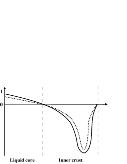
Figure 2: Rough sketch of expected radial dependence of dimensionless “operational” entrainment coefficients $\varepsilon_{\rm f}$ (dashed line) and $\varepsilon_{\rm c}$ (solid line) in a neutron star.

The link with work on the core regime can be made more explicit by using notation of the kind employed by Prix et al. [3, 5, 6, 7] in which the neutron and proton 3-momenta are given in terms of the relative 3-velocity ${{\color[rgb]{0.4,0,0.2}{\mit\Delta}}}^{i}={\color[rgb]{0.4,0,0.2}v}_{{\color[rgb]{0.6,0.4,0.0}\rm p}}^{i}-{\color[rgb]{0.4,0,0.2}v}_{{\rm n}}^{i}$ by expressions of the form

$$\color[rgb]{0,0,0}{\color[rgb]{1,0,0}\mu}^{{\rm n}}_{\,i}=\gamma_{ij}{\color[rgb]{1,0,0}m}\big{(}{\color[rgb]{0.4,0,0.2}v}_{{\rm n}}^{\,j}+\varepsilon_{\rm n}{{\color[rgb]{0.4,0,0.2}{\mit\Delta}}}^{j}\big{)}\,,\hskip 28.45274pt{\color[rgb]{1,0,0}\mu}^{{\color[rgb]{0.6,0.4,0.0}\rm p}}_{\,i}=\gamma_{ij}{\color[rgb]{1,0,0}m}\big{(}{\color[rgb]{0.4,0,0.2}v}_{{\color[rgb]{0.6,0.4,0.0}\rm p}}^{\,j}-\varepsilon_{\color[rgb]{0.6,0.4,0.0}\rm p}{{\color[rgb]{0.4,0,0.2}{\mit\Delta}}}^{j}\big{)}\,,$$ (4.24)

involving dimensionless parameters $\varepsilon_{\rm n}$ and $\varepsilon_{\color[rgb]{0.6,0.4,0.0}\rm p}$ that can be seen from (2.44)   and (4.24)   to be definable as

$$\color[rgb]{0,0,0}\varepsilon_{\rm n}=({\color[rgb]{1,0,0}m}-{\color[rgb]{1,0,0}m}_{\star}^{{\rm n}})/{\color[rgb]{1,0,0}m}\,,\hskip 28.45274pt\varepsilon_{\color[rgb]{0.6,0.4,0.0}\rm p}=({\color[rgb]{1,0,0}m}-{\color[rgb]{1,0,0}m}_{\star}^{{\color[rgb]{0.6,0.4,0.0}\rm p}})/{\color[rgb]{1,0,0}m}\,.$$ (4.25)

According to an identity of the same kind as that given by (4.19)   , these coefficients $\varepsilon_{\rm n}$ and $\varepsilon_{\color[rgb]{0.6,0.4,0.0}\rm p}$ will be related to each other, and to a density variable ${\color[rgb]{1,0,0}\alpha}$ introduced by Prix et al. [5] by

$$\color[rgb]{0,0,0}\varepsilon_{\rm n}{\color[rgb]{0,0.6,0.0}n}_{\rm n}=\varepsilon_{\color[rgb]{0.6,0.4,0.0}\rm p}{\color[rgb]{0,0.6,0.0}n}_{\color[rgb]{0.6,0.4,0.0}\rm p}=2{\color[rgb]{1,0,0}\alpha}/{\color[rgb]{1,0,0}m}\,,\hskip 28.45274pt{\color[rgb]{1,0,0}\alpha}=-\frac{{}_{1}}{{}^{2}}\,\bar{\color[rgb]{1,0,0}\rho}_{\rm np}\,.$$ (4.26)

This means in particular that for any given layer inside the star, the coefficients $\varepsilon_{\color[rgb]{0.6,0.4,0.0}\rm p}$ and $\varepsilon_{\rm n}$ both have the same sign, and it also shows that we shall have $|\varepsilon_{\rm n}|<|\varepsilon_{\color[rgb]{0.6,0.4,0.0}\rm p}|$ since the density of neutrons will always exceed the number of protons, increasing from a comparable value in the outer layers, where we shall have $\varepsilon_{\rm n}\approx\varepsilon_{\color[rgb]{0.6,0.4,0.0}\rm p},$ to a very much higher value, ${\color[rgb]{0,0.6,0.0}n}_{\rm n}\gg{\color[rgb]{0,0.6,0.0}n}_{\color[rgb]{0.6,0.4,0.0}\rm p}$ in the neutron rich core where we shall have $|\varepsilon_{\rm n}|\ll|\varepsilon_{\color[rgb]{0.6,0.4,0.0}\rm p}|.$ In terms of the proton fraction $x_{\color[rgb]{0.6,0.4,0.0}\rm p}={\color[rgb]{0,0.6,0.0}n}_{\color[rgb]{0.6,0.4,0.0}\rm p}/{\color[rgb]{0,0.6,0.0}n}_{\rm b}<1/2,$ it can be seen that an inequality of the type (4.21)   is equivalent to either of the restrictions

$$\color[rgb]{0,0,0}\varepsilon_{\rm n}<x_{\color[rgb]{0.6,0.4,0.0}\rm p}\,,\hskip 28.45274pt\varepsilon_{\color[rgb]{0.6,0.4,0.0}\rm p}<1-x_{\color[rgb]{0.6,0.4,0.0}\rm p}\,.$$ (4.27)

which evidently entails that the entrainment coefficients $\varepsilon_{\rm n}$ and $\varepsilon_{\color[rgb]{0.6,0.4,0.0}\rm p}$ must both be less than unity.

As the effective mass ${\color[rgb]{1,0,0}m}_{\star}^{\rm n}$ (and hence also ${\color[rgb]{1,0,0}m}_{\star}^{\color[rgb]{0.6,0.4,0.0}\rm p}$ ) has been found [25, 20] to be smaller than the ordinary nucleon mass ${\color[rgb]{1,0,0}m}$ in the outer core, it follows that the entrainment coefficients $\varepsilon_{\rm n}$ and $\varepsilon_{\color[rgb]{0.6,0.4,0.0}\rm p}$ will both be positive there. This contrasts with situation in the crust, where we expect the “comprehensive” effective mass ${\color[rgb]{1,0,0}m}_{\star}^{\rm n}>{\color[rgb]{1,0,0}m}$ to be larger compared with ${\color[rgb]{1,0,0}m}$ so that the coefficients $\varepsilon_{\rm n}$ and $\varepsilon_{\color[rgb]{0.6,0.4,0.0}\rm p}$ will both be negative, since we have found [16, 19] that the smaller effective mass given in a “realistic” gauge just for “conduction” neutrons with number density ${\color[rgb]{0,0.6,0.0}n}_{\rm f}$ (defined as those contributing significantly to the current) by ${\color[rgb]{1,0,0}m}_{\star}^{\rm f}={\color[rgb]{1,0,0}m}_{\star}^{\rm n}{\color[rgb]{0,0.6,0.0}n}_{\rm f}/{\color[rgb]{0,0.6,0.0}n}_{\rm n}$ will already be larger (and in some layers much larger) than the ordinary mass ${\color[rgb]{1,0,0}m}$ in the crust. It is to be observed that the negative values of $\varepsilon_{\rm n}$ and $\varepsilon_{\color[rgb]{0.6,0.4,0.0}\rm p}$ will actually diverge at the “neutron drip” transition where the “conduction” number density ${\color[rgb]{0,0.6,0.0}n}_{\rm f}$ tends to zero. These considerations are summarised on figures 1, 2, 3 and 4.

Figure 3: Rough sketch of expected radial dependence of “comprehensive” effective mass ratios ${\color[rgb]{1,0,0}m}_{\star}^{\rm n}/{\color[rgb]{1,0,0}m}$ (dashed line) and ${\color[rgb]{1,0,0}m}_{\star}^{{\color[rgb]{0.6,0.4,0.0}\rm p}}/{\color[rgb]{1,0,0}m}$ (solid line) in a neutron star.

Figure 4: Rough sketch of expected radial dependence of “operational” effective mass ratios, ${\color[rgb]{1,0,0}m}_{\star}^{\rm f}/{\color[rgb]{1,0,0}m}$ (dashed line) and ${\color[rgb]{1,0,0}m}_{\star}^{\rm c}/{\color[rgb]{1,0,0}m}$ (solid line) in a neutron star.

The total material energy density (as locally defined without allowance for gravity) will be expressible in the “comprehensive” treatment by

$$\color[rgb]{0,0,0}{\color[rgb]{1,0,0}U}_{\rm mat}=\tilde{\color[rgb]{1,0,0}U}_{\rm kin}+\tilde{\color[rgb]{1,0,0}U}_{\rm int}\,,\hskip 28.45274pt\tilde{\color[rgb]{1,0,0}U}_{\rm int}=\tilde{\color[rgb]{1,0,0}U}_{\rm ins}+\tilde{\color[rgb]{1,0,0}U}_{\rm ent}\,,$$ (4.28)

with the kinetic contribution given by the usual formula

$$\color[rgb]{0,0,0}\tilde{\color[rgb]{1,0,0}U}_{\rm kin}=\frac{{}_{1}}{{}^{2}}{\color[rgb]{1,0,0}m}\big{(}{\color[rgb]{0,0.6,0.0}n}_{\rm n}{\color[rgb]{0.4,0,0.2}v}_{\rm n}^{2}+{\color[rgb]{0,0.6,0.0}n}_{\color[rgb]{0.6,0.4,0.0}\rm p}{\color[rgb]{0.4,0,0.2}v}_{\color[rgb]{0.6,0.4,0.0}\rm p}^{2}\big{)}\,,$$ (4.29)

while from equations (2.60)   , (2.65)   and (4.25)   it can be seen that the two fluid equation of state will be expressible in terms of a pair of 3-variable functions $\tilde{\color[rgb]{1,0,0}U}_{\rm ins}\{{\color[rgb]{0,0.6,0.0}n}_{\rm I},{\color[rgb]{0,0.6,0.0}n}_{\rm n},{\color[rgb]{0,0.6,0.0}n}_{\color[rgb]{0.6,0.4,0.0}\rm p}\}$ and ${\color[rgb]{1,0,0}\alpha}\{{\color[rgb]{0,0.6,0.0}n}_{\rm I},{\color[rgb]{0,0.6,0.0}n}_{\rm n},{\color[rgb]{0,0.6,0.0}n}_{\color[rgb]{0.6,0.4,0.0}\rm p}\}$ in terms of the quantity that has been loosely referred by Prix et al. [3, 5, 6, 7] to as the “internal energy density” – but that is actually the negative of the internal action density – will be given by

$$\color[rgb]{0,0,0}-\tilde{\color[rgb]{1,0,0}\Lambda}_{\rm int}=\tilde{\color[rgb]{1,0,0}U}_{\rm ins}+{\color[rgb]{1,0,0}\alpha}\,{{\color[rgb]{0.4,0,0.2}{\mit\Delta}}}^{2}\,.$$ (4.30)

whereas the true internal energy density will be given by

$$\color[rgb]{0,0,0}\tilde{\color[rgb]{1,0,0}U}_{\rm int}=\tilde{\color[rgb]{1,0,0}U}_{\rm ins}-{\color[rgb]{1,0,0}\alpha}\,{{\color[rgb]{0.4,0,0.2}{\mit\Delta}}}^{2}\,.$$ (4.31)

In the high density core region the static energy contribution $\tilde{\color[rgb]{1,0,0}U}_{\rm ins}$ will cease to have any dependence on the ionic number density ${\color[rgb]{0,0.6,0.0}n}_{\rm I}$ , not because of any tendency of ${\color[rgb]{0,0.6,0.0}n}_{\rm I}$ to vanish on the lower boundary of the crust (where it merely ceases to be well defined) but rather because the corresponding clustering energy coefficient ${\color[rgb]{1,0,0}\mu}^{\rm I}$ will vanish there, so that the value of ${\color[rgb]{0,0.6,0.0}n}_{\rm I}$ no longer matters.

As depicted in figure 1, the entrainment coefficients between the neutron and proton fluids in the core of a neutron star are expected to be very small compared to the previously neglected entrainment coefficients in the inner crust layers. This strong entrainment in the inner crust may have significant effects on the dynamical evolution of the star. For instance, as recently shown by Andersson et al. [26], sufficiently large negative values of the entrainment coefficients $\varepsilon_{\rm n}$ and $\varepsilon_{\color[rgb]{0.6,0.4,0.0}\rm p}$ could trigger a Kelvin-Helmholtz instability in the fluid mixture which might be at the origin of observed pulsar glitches. The development of gravitational wave detectors could provide valuable constraints upon the internal structure of a neutron star by asteroseismology [27]. However a thorough understanding of the oscillation modes of a neutron star is required in order to extract useful information from the gravitational wave data. Hydrodynamical simulations of neutron star cores indicate that these oscillation modes are very sensitive to entrainment [27]. The inner crust, where the two fluids are expected to be the most strongly coupled, should therefore be given careful consideration in neutron star dynamical studies. As shown in the present work, a simple neutron star two fluid model allowing for the presence of the crust (but neglecting the stress anisotropy), can be easily implemented by suitable adjustments of the corresponding entrainment coefficients.

Acknowledgements. This work was supported by the LEA Astro-PF program. Pawel Haensel was supported by the KBN grant no. 1-P03D-008-27. Nicolas Chamel was supported by the Lavoisier program of the French Ministry of Foreign Affairs.

References

- [1] M. Ruderman, “Neutron star crustal plate tectonics: Magnetic dipole evolution in millisecond pulsars and low-mass X-ray binaries”, Astroph. J. 366 (1991) 261-269.
- [2] L. Lindblom, G. Mendell, “R modes in superfluid neutron stars” Phys.Rev. D61 (2000)104003. [gr-qc/9909084]
- [3] R.Prix, G.L. Comer, N. Andersson, “Inertial modes of non-stratified superfluid neutron stars” Mon. Not. R. Astr. Soc. 348 (2004) 652-662. [astro-ph/0308507]
- [4] G. Mendell “Superfluid hydrodynamics in rotating neutron stars. I Nondissipative equations”, Astroph. J. 380 (1991) 515-529.
- [5] R. Prix, G. L. Comer, N. Andersson, “Slowly rotating superfluid Newtonian neutron star model with entrainment”, Astron. Astrophys. 381 (2002) 178-196. [astro-ph/0107176]
- [6] R. Prix, M. Rieutord, “Adiabatic oscillations of non-rotating superfluid neutron stars”, Astron. Astroph. 393 (2002) 949-964. [ astro-ph/0204520]
- [7] R. Prix, “Variational description of multifluid hydrodynamics: uncharged fluids”, Phys. Rev. D69 (2004) 043001. [physics/0209024]
- [8] N. Andersson, G.L. Comer, K. Grosart, “Lagrangian perturbation theory of nonrelativistic rotating superfluid stars”, Mon. Not. R. Astr. Soc. 355 (2004) 918-928. [astro-ph/0402640]
- [9] B. Carter, N. Chamel, “Covariant analysis of Newtonian multifluid models for neutron stars: I Milne-Cartan structure and variational formulation”, Int. J. Mod. Phys. D13 (2004) 291-325. [astro-ph/0305186]
- [10] B. Carter, N. Chamel, “Covariant analysis of Newtonian multifluid models for neutron stars: II Stress - energy tensors and virial theorems”, Int. J. Mod. Phys. D14 (2005) 717-748. [astro-ph/0312414]
- [11] B. Carter, N. Chamel, “Covariant analysis of Newtonian multifluid models for neutron stars: III Transvective, viscous, and superfluid drag dissipation”, Int. J. Mod. Phys. D14 (2005) 749-774. [astro-ph/0410660]
- [12] D. Langlois, D. Sedrakian, B. Carter, “Differential rotation of relativistic superfluid in neutron stars”, Mon. Not. R. Astr. Soc. 297 (1998) 1198-1201. [astro-ph/9711042]
- [13] B. Carter, E. Chachoua, N. Chamel, “Covariant Newtonian and Relativistic dynamics of (magneto)-elastic solid model for neutron star crust”, Gen. Rel. Grav. 38 (2006) 83-119. [gr-qc/0507006]
- [14] B. Carter, E. Chachoua, “Newtonian mechanics of neutron superfluid in elastic star crust”, preprint. [astro-ph/0601658]
- [15] A. F. Andreev, E. P. Bashkin, “Three velocity hydrodynamics of superfluid solutions”, Sov. Phys. JETP 42 (1975) 164-167.
- [16] B. Carter, N. Chamel, P. Haensel, “Entrainment coefficient and effective mass for conduction neutrons in neutron star crust: simple microscopic models”, Nucl. Phys. A748 (2005) 675-697. [nucl-th/0402057]
- [17] K. Oyamatsu, Y. Yamada “Shell energies of non spherical nuclei in the inner crust of a neutron star”, Nucl. Phys. A578 (1994) 184-203.
- [18] B. Carter, N. Chamel, P. Haensel, “Effect of BCS pairing on entrainment in neutron superfluid current in neutron star crust”, Nucl. Phys A 759 (2005) 441-164. [astro-ph/0406228]
- [19] N. Chamel, “Band structure effects for dripped neutrons in neutron star crust”, Nucl. Phys A 747 (2005) 109-128. [ nucl-th/0405003]
- [20] G.L. Comer, R. Joynt, “A relativistic mean field model for entrainment in general relativistic superfluid neutron stars”, Phys. Rev. D68 (2003) 023002. [gr-qc/0212083]
- [21] B. Carter, D. Sedrakian, D. Langlois, “Centrifugal buoyancy as a mechanism for neutron star glitches”, Astron. Astroph., 361 (2000) 795 - 802. [astro-ph/0004121]
- [22] B. Carter, N. Chamel, “Effect of entrainment on stress and pulsar glitches in neutron star crust”, preprint. [astro-ph/0503044]
- [23] C. J. Pethick, D. G. Ravenhall, “Matter at large neutron excess and the physics of neutron star crusts”, Annu. Rev. Part. Sci. 45 (1995) 429-484.
- [24] P. Haensel, “Neutron Star Crusts” , LNP 578 Physics of Neutron Star Interiors, ed. D. Blaschke, N. K. Glendenning A. Sedrakian, (Springer 2001) 127-174.
- [25] M. Borumand, R. Joynt, W. Kluzniak, “Superfluid densities in neutron star matter”, Phys. Rev. C V54-N5 (1996) 2745-2750.
- [26] N. Andersson, G. L. Comer, R. Prix, “The superfluid two-stream instability”, Mon. Not. R. Astr. Soc. 354 (2004) 101-110.
- [27] N. Andersson, “Topical Review: Gravitational waves from instabilities in relativistic stars”, Class. Quantum Grav. 20 (2003) R105-R144. [astro-ph/0211057]