Excitation of large-scale inertial waves in a rotating inhomogeneous turbulence

Abstract

A mechanism of excitation of the large-scale inertial waves in a rotating inhomogeneous turbulence due to an excitation of a large-scale instability is found. This instability is caused by a combined effect of the inhomogeneity of the turbulence and the uniform mean rotation. The source of the large-scale instability is the energy of the small-scale turbulence. We determined the range of parameters at which the large-scale instability occurs, the growth rate of the instability and the frequency of the generated large-scale inertial waves.

I Introduction

The study of rotating flows is of interest for a wide range of problems, ranging from engineering (e.g., turbomachinery), astrophysics (galactic and accretion discs) to geophysics (oceans, the atmosphere of the Earth, gaseous planets) and weather predictions (see, e.g., P87 ; G90 ; SF97 ). Inertial waves arise in rotating flows and are observed in the atmosphere of the Earth and in laboratory rotating flows. In turbulent rotating flows inertial waves are damped due to a high turbulent viscosity. Thus, excitation of coherent and undamped inertial waves by turbulence seems not to be effective. However, large-scale inertial waves are observed in turbulent rotating flows. A mechanism of excitation of the large-scale coherent inertial waves in turbulence is not well understood.

Inertial waves are related with generation of large-scale vorticity. Generation of a large-scale vorticity in a helical turbulence due to hydrodynamical $\alpha$ effect was suggested in MST83 ; KMT91 ; CMP94 . This effect is associated with the $\alpha\tilde{\bf W}$ term in the equation for the mean vorticity, where $\tilde{\bf W}$ are the perturbations of the mean vorticity and $\alpha$ is determined by the hydrodynamical helicity of turbulent flow. A nonzero hydrodynamical helicity is caused, e.g., by a combined effect of an uniform rotation and inhomogeneity of turbulence.

Formation of large-scale vortices in a turbulent rotating flows was studied experimentally and in numerical simulations (see, e.g., ME73 ; HB82 ; ZBF97 ; TYK98 ; MK99 ; GL99 ; AK99 ). Formation of large-scale coherent structures (e.g., large-scale cyclonic and anticyclonic vortices) in a small-scale turbulence is one of the characteristic features of rotating turbulence (see, e.g., ZBF97 ). A number of mechanisms have been proposed to describe generation of a mean flow by a small-scale rotating turbulence, e.g., the effect of angular momentum mixing BT68 and vorticity expulsion GL68 . The first experimental demonstration wherein it was shown that the divergence of the Reynolds stresses can generate an organized mean circulation was described in ZBF97 .

There is a certain similarity between mean rotation and a mean velocity shear. Generation of a mean vorticity in a nonhelical homogeneous incompressible turbulent flow with an imposed mean velocity shear due to an excitation of a large-scale instability was studied in EKR03 . This instability is caused by a combined effect of the large-scale shear motions (”skew-induced” deflection of equilibrium mean vorticity) and ”Reynolds stress-induced” generation of perturbations of the mean vorticity. This instability and the dynamics of the mean vorticity are associated with the Prandtl’s turbulent secondary flows (see, e.g., P52 ; T56 ; B87 ; C94 ). However, a turbulence with an imposed mean velocity shear and a uniformly rotating turbulence are different. In particular, the mean vorticity is generated by a homogeneous nonhelical sheared turbulence EKR03 . On the other hand, the mean vorticity cannot be generated by a homogeneous uniformly rotating nonhelical turbulence (see below). The main difference between these two flows is that the mean velocity shear produces work in a turbulent flow, while a uniform rotation does not produce work in a homogeneous turbulent flow.

There are other interesting problems related with the inertial waves including, e.g., the effect of inertial waves on the onset of convection and on the turbulence dynamics. In particular, the onset of convection in the form of inertial waves in a rotating fluid sphere were studied in BS04 . On the other hand, the modification of turbulence dynamics by rotation is due to the presence of small-scale inertial waves in rotating flows (see, e.g., G90 ; CS99 ; BPS03 ; GA03 ; CR04 ).

The main goal of this paper is to study large-scale structures formed in a rotating inhomogeneous turbulence. In particular, we investigate the excitation of large-scale inertial waves. These structures are associated with a generation of a large-scale vorticity due to the excitation of the large-scale instability in an uniformly rotating inhomogeneous turbulence. The excitation of the mean vorticity in this system requires an inhomogeneity of turbulence.

This paper is organized as follows. In Section II we formulated the governing equations, the assumptions and the procedure of the derivation. In Section III the effective force was determined, which allowed us to derive the mean-filed equations and to study the excitation of large-scale inertial waves in Section IV. The large-scale instability was investigated in Section IV analytically for a weakly inhomogeneous turbulence and numerically for an arbitrary inhomogeneous turbulence. Conclusions and applications of the obtained results are discussed in Section V. In Appendixes A, B and C the detailed derivation of the effective force is performed.

II The governing equations

The system of equations for the evolution of the velocity ${\bf v}$ and vorticity ${\bf W}\equiv\mbox{\boldmath$\nabla$}{\bf\times}{\bf v}$ reads:

$$\biggl{[}{\partial\over\partial t}+{\bf v}\cdot\mbox{\boldmath$\nabla$}\biggr{]}{\bf v}=-{\mbox{\boldmath$\nabla$}P\over\rho}+2\,{\bf v}{\bf\times}{\bf\Omega}+\nu\Delta{\bf v}+{\bf F}_{\rm st}\;,$$ (1)

$${\partial{\bf W}\over\partial t}=\mbox{\boldmath$\nabla$}{\bf\times}\,({\bf v}{\bf\times}{\bf W}+2\,{\bf v}{\bf\times}{\bf\Omega}-\nu\mbox{\boldmath$\nabla$}{\bf\times}{\bf W})\;,$$ (2)

where ${\bf v}$ is the fluid velocity with $\mbox{\boldmath$\nabla$}\cdot{\bf v}=0,$ $\,P$ is the fluid pressure, $\,{\bf F}_{\rm st}$ is an external stirring force with a zero mean value, ${\bf\Omega}$ is a constant angular velocity and $\nu$ is the kinematic viscosity. Equation (2) follows from the Navier-Stokes equation (1). We use a mean field approach whereby the velocity, pressure and vorticity are separated into the mean and fluctuating parts: ${\bf v}=\bar{\bf U}+{\bf u},$ $P=\bar{P}+p$ and ${\bf W}=\bar{\bf W}+{\bf w},$ the fluctuating parts have zero mean values, $\bar{\bf U}=\langle{\bf v}\rangle,$ $\,\bar{P}=\langle P\rangle$ and $\bar{{\bf W}}=\langle{\bf W}\rangle.$ Averaging Eqs. (1) and (2) over an ensemble of fluctuations we obtain the equations for the mean velocity $\bar{\bf U}$ and mean vorticity $\bar{{\bf W}}:$

$$\biggl{[}{\partial\over\partial t}+\bar{\bf U}\cdot\mbox{\boldmath$\nabla$}\biggr{]}\bar{\bf U}=-{\mbox{\boldmath$\nabla$}\bar{P}\over\rho}+2\,\bar{\bf U}{\bf\times}{\bf\Omega}+\mbox{\boldmath$\cal F$}+\nu\Delta\bar{\bf U}\;,$$ (3)

$${\partial\bar{{\bf W}}\over\partial t}=\mbox{\boldmath$\nabla$}{\bf\times}\,(\bar{\bf U}{\bf\times}\bar{{\bf W}}+2\,\bar{\bf U}{\bf\times}{\bf\Omega}+\langle{\bf u}{\bf\times}{\bf w}\rangle-\nu\mbox{\boldmath$\nabla$}{\bf\times}\bar{{\bf W}})\;,$$ (4)

where ${\cal F}_{i}=-\nabla_{j}\langle u_{i}u_{j}\rangle.$ Note that the effect of turbulence on the mean vorticity is determined by the Reynolds stresses $\langle u_{i}u_{j}\rangle$ because

$$\langle{\bf u}{\bf\times}{\bf w}\rangle_{i}=-\nabla_{j}\langle u_{i}u_{j}\rangle+{1\over 2}\nabla_{i}\langle{\bf u}^{2}\rangle\;.$$ (5)

Consider a steady state solution of Eqs. (3) and (4) in the form: $\bar{\bf U}^{(s)}=0$ and $\bar{\bf W}^{(s)}=0.$ In order to study a stability of this equilibrium we consider perturbations of the mean velocity, $\tilde{\bf U},$ and the mean vorticity, $\tilde{{\bf W}}.$ The linearized equations for the small perturbations of the mean velocity and the mean vorticity are given by

$${\partial\tilde{\bf U}\over\partial t}=-{\mbox{\boldmath$\nabla$}\tilde{P}\over\rho}+2\,\tilde{\bf U}{\bf\times}{\bf\Omega}+\tilde{\mbox{\boldmath$\cal F$}}(\tilde{\bf U})+\nu\Delta\tilde{\bf U}\;,$$ (6)

$${\partial\tilde{\bf W}\over\partial t}=\mbox{\boldmath$\nabla$}{\bf\times}\,(2\,\tilde{\bf U}{\bf\times}\mbox{\boldmath$\Omega$}+\tilde{\mbox{\boldmath$\cal F$}}(\tilde{\bf U})-\nu\mbox{\boldmath$\nabla$}{\bf\times}\tilde{{\bf W}})\;,$$ (7)

where $\tilde{\mbox{\boldmath$\cal F$}}(\tilde{\bf U})=-\nabla_{j}(f_{ij}-f_{ij}^{(0)})$ is the effective force, $f_{ij}=\langle u_{i}u_{j}\rangle$ and $f_{ij}^{(0)}$ is the second moment of the velocity field in a background turbulence (with a zero gradient of the mean velocity). Thus, the mean fields $\tilde{\bf U}$ and $\tilde{\bf W}$ represent deviations from the equilibrium solution $\bar{\bf U}^{(s)}=0$ and $\bar{\bf W}^{(s)}=0.$ This equilibrium solution is a steady state solution of Eqs. (3) and (4). Note that the characteristic times and spatial scales of small-scale fluctuations of velocity and vorticity ${\bf u}$ and ${\bf w}$ are much smaller than that of the mean fields $\tilde{\bf U}$ and $\tilde{\bf W}$.

In order to obtain a closed system of equations in the next Section we derived an equation for the effective force $\tilde{\mbox{\boldmath$\cal F$}}.$

III The effective force

In this section we derive an equation for the effective force $\tilde{\mbox{\boldmath$\cal F$}}.$ The mean velocity gradients can affect turbulence. The reason is that additional essentially non-isotropic velocity fluctuations can be generated by tangling of the mean-velocity gradients with the Kolmogorov-type turbulence. The source of energy of this ”tangling turbulence” is the energy of the Kolmogorov turbulence. The tangling turbulence was introduced by Wheelon W57 and Batchelor et al. BH59 for a passive scalar and by Golitsyn G60 and Moffatt M61 for a passive vector (magnetic field). Anisotropic fluctuations of a passive scalar (e.g., the number density of particles or temperature) are generated by tangling of gradients of the mean passive scalar field with a random velocity field. Similarly, anisotropic magnetic fluctuations are excited by tangling of the mean magnetic field with the velocity fluctuations. The Reynolds stresses in a turbulent flow with mean velocity gradients is another example of a tangling turbulence. Indeed, they are strongly anisotropic in the presence of mean velocity gradients and have a steeper spectrum $(\propto k^{-7/3})$ than a Kolmogorov turbulence (see, e.g., L67 ; WC72 ; SV94 ; IY02 ; EKRZ02 ). The anisotropic velocity fluctuations of tangling turbulence were studied first by Lumley L67 .

To derive an equation for the effective force $\tilde{\mbox{\boldmath$\cal F$}}$ we use equation for fluctuations ${\bf u}(t,{\bf r})$ which is obtained by subtracting Eq. (3) for the mean field from Eq. (1) for the total field:

$${\partial{\bf u}\over\partial t} = -(\bar{\bf U}\cdot\mbox{\boldmath$\nabla$}){\bf u}-({\bf u}\cdot\mbox{\boldmath$\nabla$})\bar{\bf U}-{\mbox{\boldmath$\nabla$}p\over\rho}$$ (8)

$$+2\,{\bf u}{\bf\times}\mbox{\boldmath$\Omega$}+{\bf F}_{\rm st}+{\bf U}^{N}\;,$$

where

$${\bf U}^{N} = \langle({\bf u}\cdot\mbox{\boldmath$\nabla$}){\bf u}\rangle-({\bf u}\cdot\mbox{\boldmath$\nabla$}){\bf u}+\nu\Delta{\bf u}\;.$$ (9)

We consider a turbulent flow with large Reynolds numbers $({\rm Re}=l_{0}u_{0}/\nu\gg 1)$, where $u_{0}$ is the characteristic velocity in the maximum scale $l_{0}$ of turbulent motions. We assume that there is a separation of scales, i.e., the maximum scale of turbulent motions $l_{0}$ is much smaller then the characteristic scale of inhomogeneities of the mean fields. Using Eq. (8) we derived equation for the second moment of turbulent velocity field $f_{ij}({\bf k,R})\equiv\int\langle u_{i}({\bf k}+{\bf K}/2)u_{j}(-{\bf k}+{\bf K}/2)\rangle\exp(i{\bf K}{\bf\cdot}{\bf R})\,d{\bf K}$:

$${\partial f_{ij}({\bf k,R})\over\partial t} = {\cal G}_{ijmn}f_{mn}+F_{ij}+f_{ij}^{(N)}\;$$ (10)

(see Appendix A), where ${\cal G}_{ijmn}=I_{ijmn}(\tilde{\bf U})+N_{ijmn}({\bf\Omega}),$

$$I_{ijmn}(\tilde{\bf U}) = \biggl{[}2k_{iq}\delta_{mp}\delta_{jn}+2k_{jq}\delta_{im}\delta_{pn}-\delta_{im}\delta_{jq}\delta_{np}$$ (11)

$$-\delta_{iq}\delta_{jn}\delta_{mp}+\delta_{im}\delta_{jn}k_{q}{\partial\over\partial k_{p}}\biggr{]}\nabla_{p}\tilde{U}_{q}\;,$$

$$N_{ijmn}({\bf\Omega}) = 2\,\Omega_{q}k_{pq}(\varepsilon_{imp}\,\delta_{nj}+\varepsilon_{jmp}\,\delta_{ni})\;,$$ (12)

and ${\bf R}$ and ${\bf K}$ correspond to the large scales, and ${\bf r}$ and ${\bf k}$ to the small scales (see Appendix A), $\delta_{ij}$ is the Kronecker tensor, $k_{ij}=k_{i}k_{j}/k^{2},$ and $\mbox{\boldmath$\nabla$}=\partial/\partial{\bf R},$ $\,F_{ij}({\bf k},{\bf R})=\langle\tilde{F}_{i}({\bf k},{\bf R})u_{j}(-{\bf k},{\bf R})\rangle+\langle u_{i}({\bf k},{\bf R})\tilde{F}_{j}(-{\bf k},{\bf R})\rangle$, $\,{\bf\tilde{F}}({\bf k},{\bf R},t)=-{\bf k}{\bf\times}({\bf k}{\bf\times}{\bf F}_{\rm st}({\bf k},{\bf R}))/k^{2}$ and $f_{ij}^{(N)}({\bf k},{\bf R})$ are the terms which are related with the third moments appearing due to the nonlinear terms. The third moments terms $f_{ij}^{(N)}$ are defined as

$$f_{ij}^{(N)}({\bf k},{\bf R}) = \langle P_{in}({\bf k}_{1})\hat{U}^{N}_{n}({\bf k}_{1})u_{j}({\bf k}_{2})\rangle$$

$$+\langle u_{i}({\bf k}_{1})P_{jn}({\bf k}_{2})\hat{U}^{N}_{n}({\bf k}_{2})\rangle\;,$$

where $\hat{\bf U}^{N}_{n}({\bf k})$ is the Fourier transform of ${\bf U}^{N}$ determined by Eq. (9), ${\bf k}_{1}={\bf k}+{\bf K}/2$, $\,{\bf k}_{2}=-{\bf k}+{\bf K}/2$ and $P_{ij}({\bf k})=\delta_{ij}-k_{ij}$.

Equation (10) is written in a frame moving with a local velocity $\tilde{\bf U}$ of the mean flow. In Eq. (10) for the second moments of the turbulent velocity field we neglected small terms $\sim O(\nabla^{2})$ , where the terms with $\nabla\sim O(L^{-1})$ contain the large-scale spatial derivatives. These terms are of the order of $(l_{0}/L)^{2}$, where the maximum scale of turbulent motions $l_{0}$ is much smaller than the vertical size of the turbulent region $L$.

Equation (10) for the background turbulence (with a zero gradient of the mean fluid velocity $\nabla_{i}\tilde{U}_{j}=0$ and ${\bf\Omega}=0)$ reads

$${\partial f_{ij}^{(0)}({\bf k,R})\over\partial t}=F_{ij}+f_{ij}^{(N,0)}\;,$$ (13)

where the superscript ${(0)}$ corresponds to the background turbulence, and we assumed that the tensor $F_{ij}({\bf k,R}),$ which is determined by a stirring force, is independent of the mean velocity gradients and of a constant mean angular velocity. Equation for the deviations $f_{ij}-f_{ij}^{(0)}$ from the background turbulence is given by

$${\partial(f_{ij}-f_{ij}^{(0)})\over\partial t}={\cal G}_{ijmn}f_{mn}+f_{ij}^{(N)}-f_{ij}^{(N,0)}\;.$$ (14)

Equation (14) for the deviations of the second moments $f_{ij}-f_{ij}^{(0)}$ in ${\bf k}$-space contains the deviations of the third moments $f_{ij}^{(N)}-f_{ij}^{(N,0)}$ and a problem of closing the equations for the higher moments arises. Various approximate methods have been proposed for the solution of problems of this type (see, e.g., MY75 ; O70 ; Mc90 ). The simplest procedure is the $\tau$ approximation which was widely used for study of different problems of turbulent transport (see, e.g., O70 ; PFL76 ; KRR90 ; RK2000 ; BK04 ). One of the simplest procedures, that allows us to express the deviations of the terms with the third moments $f_{ij}^{(N)}-f_{ij}^{(N,0)}$ in ${\bf k}$-space in terms of that for the second moments $f_{ij}-f_{ij}^{(0)},$ reads

$$f_{ij}^{(N)}-f_{ij}^{(N,0)} = -{f_{ij}-f_{ij}^{(0)}\over\tau(k)}\;,$$ (15)

where $\tau(k)$ is the scale dependent correlation time of the turbulent velocity field. Here we assumed that the time $\tau(k)$ is independent of the mean velocity gradients (for a weak mean velocity shear). We considered also the case of slow rotation rate. In this case a modification of the correlation time of fully developed turbulence by slow rotation is small. This allows us to suggest that Eq. (15) is valid for a slow rotation rate.

The $\tau$-approximation is different from Eddy Damped Quasi Normal Markowian (EDQNM) approximation. A principle difference between these two approaches is as follows (see O70 ; Mc90 ). The EDQNM closures do not relax to the equilibrium, and this procedure does not describe properly the motions in the equilibrium state. In EDQNM approximation, there is no dynamically determined relaxation time, and no slightly perturbed steady state can be approached O70 . In the $\tau$-approximation, the relaxation time for small departures from equilibrium is determined by the random motions in the equilibrium state, but not by the departure from equilibrium O70 . Analysis performed in O70 showed that the $\tau$-approximation describes the relaxation to the equilibrium state (the background turbulence) more accurately than the EDQNM approach.

Note that we applied the $\tau$-approximation (15) only to study the deviations from the background turbulence which are caused by the spatial derivatives of the mean velocity and a uniform rotation. The background turbulence is assumed to be known. Here we use the following model for the background isotropic and weakly inhomogeneous turbulence:

$$f^{(0)}_{ij}({\bf k},{\bf R}) = \frac{{\cal E}(k)}{8\pi k^{2}}\biggl{[}P_{ij}({\bf k})+\frac{i}{2k^{2}}(k_{i}\nabla_{j}$$ (16)

$$-k_{j}\nabla_{i})\biggr{]}\langle{\bf u}^{2}\rangle^{(0)}\;$$

(see e.g., EKR95 ), where $P_{ij}({\bf k})=\delta_{ij}-k_{ij}$, $\,\delta_{ij}$ is the Kronecker tensor and $k_{ij}=k_{i}k_{j}/k^{2}$, $\,\tau(k)=2\tau_{0}\bar{\tau}(k),$ $\,{\cal E}(k)=-d\bar{\tau}(k)/dk,$ $\,\bar{\tau}(k)=(k/k_{0})^{1-q},$ $\,1<q<3$ is the exponent of the kinetic energy spectrum (e.g., $q=5/3$ for Kolmogorov spectrum), $k_{0}=1/l_{0}.$

The mean velocity gradient $\nabla_{i}\tilde{\bf U}$ causes generation of anisotropic velocity fluctuations (tangling turbulence). Equations (14)-(16) allow to determine the second moment $f_{ij}({\bf R})=\int f_{ij}({\bf k},{\bf R})\,d{\bf k}$:

$$f_{ij}({\bf R}) = f_{ij}^{(0)}({\bf R})-\nu_{{}_{T}}^{(0)}M_{ij}-{1\over 6}l_{0}^{2}\,\Omega S_{ij}\;$$ (17)

(see Appendix B), where $\nu_{{}_{T}}^{(0)}=\tau_{0}\langle{\bf u}^{2}\rangle^{(0)}/6$ and the tensors $M_{ij}$ and $S_{ij}$ are determined in Appendix B. The definition of the function $\nu_{{}_{T}}^{(0)}$ yields $\langle{\bf u}^{2}\rangle^{(0)}({\bf R})=6\nu_{{}_{T}}^{(0)}({\bf R})/\tau_{0}$. Since we assumed that $\tau_{0}$ is independent of ${\bf R}$, the spatial profile of the function $\nu_{{}_{T}}^{(0)}$ [e.g., given by Eq. (LABEL:PB1) in Sect. IV-B] determines the spatial profile of $\langle{\bf u}^{2}\rangle^{(0)}$. Equation (17) allows to determine the effective force $\tilde{\cal F}_{i}=-{\nabla}_{j}[f_{ij}({\bf R})-f_{ij}^{(0)}({\bf R})]:$

$$\tilde{\cal F}_{i}=\nu_{{}_{T}}^{(0)}(M_{ij}\Lambda_{j}+\nabla_{j}M_{ij})+{1\over 6}l_{0}^{2}\,\Omega(S_{ij}\Lambda_{j}+\nabla_{j}S_{ij})\;,$$

(18)

where ${\bf\Lambda}=(\mbox{\boldmath$\nabla$}l_{0}^{2})/l_{0}^{2}=(\mbox{\boldmath$\nabla$}\nu_{{}_{T}}^{(0)})/\nu_{{}_{T}}^{(0)}.$

Note that when $\Lambda=const,$ the effective force $\tilde{\mbox{\boldmath$\cal F$}}$ does not have the term $\propto\alpha\tilde{\bf W},$ where $\alpha$ describes the hydrodynamic $\alpha$-effect. The hydrodynamic $\alpha$-effect was introduced in the equation for the mean vorticity (see, e.g., MST83 ; KMT91 ; CMP94 ), similarly to the $\alpha$-effect in the equation for the evolution of the mean magnetic field (see, e.g., M78 ). The reason for the absence of the $\alpha\tilde{\bf W}$ term in $\tilde{\mbox{\boldmath$\cal F$}}$ is as follows. Let us suggest the opposite, i.e., that $\tilde{\mbox{\boldmath$\cal F$}}\propto\alpha\tilde{\bf W}=\alpha\mbox{\boldmath$\nabla$}{\bf\times}\tilde{\bf U}.$ Since the effective force $\tilde{\cal F}_{i}=-{\nabla}_{j}[f_{ij}({\bf R})-f_{ij}^{(0)}({\bf R})],$ we obtain

$$f_{ij}({\bf R})-f_{ij}^{(0)}({\bf R})\propto-\alpha\varepsilon_{ijk}\tilde{U}_{k}\;.$$ (19)

Here we used the identity $\tilde{W}_{i}=\varepsilon_{ijk}\nabla_{j}\tilde{U}_{k}$ and we took into account that when $\Lambda=const,$ the hydrodynamic $\alpha$ is constant. Note also that in our paper we considered incompressible velocity field. The condition (19) is in contradiction with the Galilean invariance, because the Reynolds stresses in the considered case may depend on the gradient of the mean velocity field rather than on the mean velocity itself. When $\Lambda$ is not constant, the effective force $\tilde{\mbox{\boldmath$\cal F$}}$ can have the term $\propto\alpha\tilde{\bf W}.$ However, this effect is not in the scope of our paper (e.g., this case cannot be described in the framework of the gradient approximation).

IV The large-scale instability in an inhomogeneous turbulence

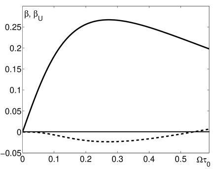
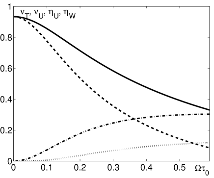
Figure 1: The rotation rate dependence of the functions $\beta(\Omega\tau_{0})$ (solid) and $\beta_{{}_{U}}(\Omega\tau_{0})$ (dashed).

Figure 2: The rotation rate dependence of the functions $\nu_{{}_{T}}(\Omega\tau_{0})$ (solid), $\nu_{{}_{U}}(\Omega\tau_{0})$ (dashed-dotted), $\eta_{{}_{W}}(\Omega\tau_{0})$ (dashed) and $\eta_{{}_{U}}(\Omega\tau_{0})$ (dotted).

For simplicity we consider the case when the turbulence is inhomogeneous along the rotation axis, i.e., ${\bf\Lambda}=\Lambda(z){\bf e}_{z},$ $\,{\bf\Omega}=\Omega{\bf e}_{z}.$ After calculating $[\mbox{\boldmath$\nabla$}{\bf\times}(\mbox{\boldmath$\nabla$}{\bf\times}\tilde{\bf U})]_{z}$ from Eq. (6) and $\tilde{W}_{z}$ from Eq. (7) we arrive at the following equations written in nondimensional form

$$\Delta{\partial\tilde{U}_{z}\over\partial t} = -[\hat{G}-\beta_{{}_{U}}\,\Delta_{\perp}\nabla_{z}]\,\tilde{W}_{z}+[\nu_{{}_{T}}\,\Delta^{2}+\nu_{{}_{T}}\,\Lambda\,\Delta\,\nabla_{z}$$ (20)

$$+\,\nu_{{}_{U}}\,\Lambda\,\Delta_{\perp}\,\nabla_{z}+\eta_{{}_{U}}\,\Delta_{\perp}\nabla_{z}^{2}]\tilde{U}_{z}\;,$$

$${\partial\tilde{W}_{z}\over\partial t} = (\hat{G}-\beta\,\Lambda\,\Delta_{\perp})\tilde{U}_{z}+[\nu_{{}_{T}}\,\nabla_{z}^{2}+\nu_{{}_{T}}\,\Lambda\,\nabla_{z}$$ (21)

$$+\,\eta_{{}_{W}}\,\Delta_{\perp}]\tilde{W}_{z}\;,$$

where $\Delta=\Delta_{\perp}+\nabla_{z}^{2}$, $\,\nabla_{z}=\partial/\partial z$,

$$\hat{G}=2\,a_{\ast}\,\nabla_{z}+\beta[\Lambda\,\nabla_{z}^{2}+\Delta\nabla_{z}]\;,$$

$$\beta(\Omega,z) = \nu_{{}_{T}}^{(0)}(z)(\omega/8)[D_{5}(\omega)/2-D_{6}(\omega)]\;,$$

$$\beta_{{}_{U}}(\Omega,z) = \nu_{{}_{T}}^{(0)}(z)(\omega/8)D_{6}(\omega)\;,$$

$$\nu_{{}_{T}}(\Omega,z) = \nu_{{}_{T}}^{(0)}(z)[D_{1}(\omega)/2+D_{2}(\omega)]\;,$$

$$\nu_{{}_{U}}(\Omega,z) = \,\eta_{{}_{U}}(\Omega,z)+2\nu_{{}_{T}}^{(0)}(z)D_{2}(\omega)\;,$$

$$\eta_{{}_{U}}(\Omega,z) = \nu_{{}_{T}}^{(0)}(z)D_{4}(\omega)\;,$$

$$\eta_{{}_{W}}(\Omega,z) = \nu_{{}_{T}}^{(0)}(z)[D_{1}(\omega)/2-D_{3}(\omega)]\;.$$

Here $\omega=8\tau_{0}\Omega,$ $\,a_{\ast}=\Omega L^{2}/\nu_{{}_{T}}^{\ast}\gg 1$, and we used Eq. (18). The functions $D_{k}(\omega)$ are determined in Appendix B.

In Eqs. (20) and (21) we use the following dimensionless variables: length is measured in units of $L$, time in units of $L^{2}/\nu_{{}_{T}}^{\ast},$ the function $\Lambda(z)$ is measured in the units of $L^{-1}$, the function $\nu_{{}_{T}}^{(0)}(z)$ is measured in the units of $\nu_{{}_{T}}^{\ast}$, the perturbations of velocity $\tilde{U}_{z}$ and vorticity $\tilde{W}_{z}$ are measured in units of $U_{\ast}$ and $U_{\ast}/L,$ respectively. The functions $\,\beta(\Omega\tau_{0})$, $\,\beta_{{}_{U}}(\Omega\tau_{0})$, $\,\nu_{{}_{T}}(\Omega\tau_{0})$, $\,\nu_{{}_{U}}(\Omega\tau_{0})$, $\,\eta_{{}_{W}}(\Omega\tau_{0})$ and $\,\eta_{{}_{U}}(\Omega\tau_{0})$ are shown in FIGS. 1-2. All these functions shown in FIGS. 1-2 are normalized by $\nu_{{}_{T}}^{(0)}(z)$, e.g, $\nu_{{}_{T}}(\Omega\tau_{0})\equiv\nu_{{}_{T}}(\Omega,z)/\nu_{{}_{T}}^{(0)}(z)$, and similarly for other functions.

IV.1 The weakly inhomogeneous turbulence

Assume that functions $\nu_{{}_{T}}^{(0)}(z)$ and $\Lambda(z)$ vary slowly with $z$ in comparison with the variations of the mean velocity $\tilde{U}_{z}(z)$ and mean vorticity $\tilde{W}_{z}(z)$. Let us seek for the solution of Eqs. (20) and (21) in the form $\propto\exp(\gamma t-i{\bf K}\cdot{\bf R}).$ Let us first consider perturbations with the wave numbers $K^{2}_{\perp}\ll K^{2}_{z}.$ Since $\mbox{\boldmath$\nabla$}\cdot\tilde{\bf U}=0,$ the velocity components $\tilde{U}_{z}\ll|\tilde{\bf U}_{\perp}|.$ Thus the growth rate of the inertial waves with the frequency

$$\omega_{w}=-{\rm sgn}(\beta\,\Lambda)\,{2\,a_{\ast}\,K_{z}\over K}\;,$$ (22)

is given by

$$\gamma_{w} = |\beta(\Omega\tau_{0})\,\Lambda\,K_{z}|-\nu_{{}_{T}}(\Omega\tau_{0})K^{2}\;,$$ (23)

where $\gamma=\gamma_{w}+i\omega_{w},$ the wave number $K$ is measured in the units of $L^{-1}$ and $\gamma$ is measured in the units of $\nu_{{}_{T}}^{\ast}/L^{2}.$ The maximum growth rate of the inertial waves, $\gamma_{m}=[\beta(\Omega\tau_{0})\,\Lambda]^{2}/4\nu_{{}_{T}}(\Omega\tau_{0}),$ is attained at $K=K_{m}=|\beta(\Omega\tau_{0})\,\Lambda|/2\nu_{{}_{T}}(\Omega\tau_{0}).$ For a very small rotation rate, i.e., for $\omega\equiv 8\Omega\tau_{0}\ll 1,$ the turbulent viscosity $\nu_{{}_{T}}(\Omega\tau_{0})\approx(q+3)/5$ and $\beta(\Omega\tau_{0})\approx(32/15)\Omega\tau_{0},$ where the parameter $q$ is the exponent of the kinetic energy spectrum of the background isotropic and weakly inhomogeneous turbulence (e.g., $q=5/3$ for Kolmogorov spectrum), and this parameter varies in the range $1<q<3$. Note that the inertial waves are helical, i.e., the large-scale hydrodynamic helicity of the motions in the inertial waves is $\tilde{\bf U}\cdot(\mbox{\boldmath$\nabla$}{\bf\times}\tilde{\bf U})=2|\tilde{\bf U}_{\perp}|^{2}K_{z}\not=0.$ This instability is caused by a combined effect of the inhomogeneity of the turbulence and the uniform mean rotation [see the first term in Eq. (23)].

Now we consider the opposite case, i.e., the perturbations with the wave numbers $K^{2}_{\perp}\gg K^{2}_{z}.$ Since $\mbox{\boldmath$\nabla$}\cdot\tilde{\bf U}=0,$ the velocity components $\tilde{U}_{z}\gg|\tilde{\bf U}_{\perp}|.$ When $K^{2}\,|\beta(\Omega)\,\Lambda|/4a_{\ast}\ll K_{z}\ll K_{\perp}$, the growth rate of perturbations with the frequency

$$\omega_{w}={\rm sgn}(\beta\,\Lambda)\,{2\,a_{\ast}\,K_{z}\over K}\;,$$ (24)

is given by

$$\gamma_{w} = {1\over 2}\biggl{[}|\beta(\Omega\tau_{0})\,\Lambda|\,K-[\nu_{{}_{T}}(\Omega\tau_{0})+\eta_{{}_{W}}(\Omega\tau_{0})]\,K^{2}\biggr{]}.$$

The maximum growth rate of perturbations, $\gamma_{m}=[\beta(\Omega\tau_{0})\,\Lambda]^{2}/8[\nu_{{}_{T}}(\Omega\tau_{0})+\eta_{{}_{W}}(\Omega\tau_{0})],$ is attained at $K=K_{m}=|\beta(\Omega\tau_{0})\,\Lambda|/2[\nu_{{}_{T}}(\Omega\tau_{0})+\eta_{{}_{W}}(\Omega\tau_{0})].$ This case corresponds to $a_{\ast}\gg\beta^{2}(\Omega\tau_{0})/4\nu_{{}_{T}}(\Omega\tau_{0}).$ The large-scale hydrodynamic helicity of the flow is $\tilde{\bf U}\cdot(\mbox{\boldmath$\nabla$}{\bf\times}\tilde{\bf U})=4K_{\perp}|\tilde{\bf U}_{z}|^{2}\,{\rm sgn}(\beta)\not=0.$

IV.2 Numerical results

In this Section we take into account the inhomogeneity of the functions $\nu_{{}_{T}}^{(0)}(z)$ and $\Lambda(z)$. We introduce a new variable $V=\Delta\tilde{U}_{z}$ and consider an eigenvalue problem for a system of Eqs. (20) and (21). We seek for a solution of Eqs. (20) and (21) in the form $\propto\Psi(z)\exp(\gamma t)J_{0}(K_{\perp}\,r),$ where $J_{0}(x)$ is the Bessel function of the first kind. After the substitution of this solution into Eqs. (20) and (21) we obtain the system of the ordinary differential equations which is solved numerically.

We used the cylindrical geometry $(z,r,\phi)$ with $z$-axis along the rotation axis and consider the axisymmetric solution (i.e., there are no derivatives with respect to the polar angle $\phi$). The turbulence is inhomogeneous along the rotation axis. We use the periodic boundary conditions in $z$ direction for Eqs. (20) and (21), i.e., $\tilde{U}_{z}(z=0,r)=\tilde{U}_{z}(z=L,r)$, $\tilde{U}_{z}^{\prime}(z=0,r)=\tilde{U}_{z}^{\prime}(z=L,r)$, $\tilde{U}_{z}^{\prime\prime}(z=0,r)=\tilde{U}_{z}^{\prime\prime}(z=L,r)$, $\tilde{U}_{z}^{\prime\prime\prime}(z=0,r)=\tilde{U}_{z}^{\prime\prime\prime}(z=L,r)$, $\tilde{W}_{z}(z=0,r)=\tilde{W}_{z}(z=L,r)$ and $\tilde{W}_{z}^{\prime}(z=0,r)=\tilde{W}_{z}^{\prime}(z=L,r)$, where $\tilde{U}^{\prime}=\nabla_{z}\tilde{U}$. We also use the condition $\tilde{U}_{r}(z,r=0)=\tilde{U}_{r}(z,r=R)=0$, where $R$ is the radius of the turbulent region.

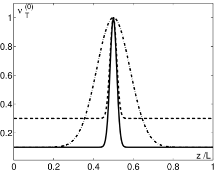
We have chosen the vertical profile of the function $\nu_{{}_{T}}^{(0)}(z)$ in the following form

$$\nu_{{}_{T}}^{(0)}(z) = 1-C\,\biggl{\{}1-\exp\biggl{[}-2\Lambda_{0}^{2}\biggl{(}\frac{z}{L}-\frac{1}{2}\biggr{)}^{2}\biggr{]}\biggr{\}}\;,$$

$$C = {1-\nu_{{}_{T}}^{(b)}\over 1-\exp(-\Lambda_{0}^{2}/2)}\;,$$

with two values of the parameter $\nu_{{}_{T}}^{(b)}=$ $\,0.1$ and $0.3$; and two values of the parameter $\Lambda_{0}=$ $\,12$ and $30$. The vertical profile of the turbulent viscosity $\nu_{{}_{T}}^{(0)}(z)$ is shown in FIG. 3. The maximum of turbulence intensity is located at $z=L/2$. The form of the chosen spatial profile of the function $\nu_{{}_{T}}^{(0)}(z)$ is simple enough and universal. It allows us to vary the size of the region occupied by turbulence (by changing the parameter $\Lambda_{0}$) and the difference in the level of the turbulence between the center and boundary of the region (by changing the parameter $\nu_{{}_{T}}^{(b)}$), i.e., it allows us to change the inhomogeneity of the turbulence. The numerical solution of Eqs.  (20) and (21) was performed also for other spatial profiles of the function $\nu_{{}_{T}}^{(0)}(z)$. However, the final results do not depend strongly on the details in the spatial profile of the function $\nu_{{}_{T}}^{(0)}(z)$. Note also that the chosen spatial profile of the function $\nu_{{}_{T}}^{(0)}(z)$ can mimic the distribution of turbulence in galactic and accretion discs (see, e.g., RSS88 ).

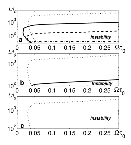
Figure 3: The vertical profile of the turbulent viscosity $\nu_{{}_{T}}^{(0)}(z)$ for $\Lambda_{0}=30$ and $\nu_{{}_{T}}^{(b)}=0.1$ (solid); $\Lambda_{0}=30$ and $\,\nu_{{}_{T}}^{(b)}=0.3$ (dashed); $\Lambda_{0}=12$ and $\,\nu_{{}_{T}}^{(b)}=0.1$ (dashed-dotted).

Figure 4: The range of parameters $(L/l_{0},\Omega\tau_{0})$ for which the large-scale instability occurs $(\gamma_{w}>0)$ for (a). $\Lambda_{0}=12$, $\,\nu_{{}_{T}}^{(b)}=0.1$; (b). $\Lambda_{0}=30$, $\,\nu_{{}_{T}}^{(b)}=0.1$; (c). $\Lambda_{0}=30$, $\,\nu_{{}_{T}}^{(b)}=0.3$; and different values of the parameter $\mu$: $\,\,\mu=0.1$ (dotted), $\mu=0.5$ (solid), $\mu=1$ (dashed), $\mu=2$ (dashed-dotted).

Figure 5: The rotation rate $(\Omega\tau_{0})$ dependencies of (a) the growth rate $\gamma_{w}\tau_{{}_{D}}$ of the large-scale instability and (b) the frequency $\omega_{w}\tau_{0}$ of the generated waves due to the large-scale instability for $\Lambda_{0}=12$, $\,\nu_{{}_{T}}^{(b)}=0.1$, $\,\mu=0.1$ and different values of the parameter $L/l_{0}$: $\,\,L/l_{0}=50$ (solid), $\,\,L/l_{0}=100$ (dashed) and $\,\,L/l_{0}=500$ (dashed-dotted). Here $\tau_{{}_{D}}=L^{2}/\nu_{{}_{T}}^{\ast}.$

Figure 6: The rotation rate $(\Omega\tau_{0})$ dependencies of (a) the growth rate $\gamma_{w}\tau_{{}_{D}}$ of the large-scale instability and (b) the frequency $\omega_{w}\tau_{0}$ of the generated waves due to the large-scale instability for $\Lambda_{0}=30$, $\,\nu_{{}_{T}}^{(b)}=0.1$, $\,\mu=0.1$ and different values of the parameter $L/l_{0}$: $\,\,L/l_{0}=100$ (solid), $\,\,L/l_{0}=500$ (dashed) and $\,\,L/l_{0}=1000$ (dashed-dotted).

The sufficient condition for the excitation of the instability is $\gamma_{w}>0$. The range of parameters $(L/l_{0},\Omega\tau_{0})$ for which the large-scale instability occurs is shown in FIG. 4 for different values of the parameters $\mu$, $\nu_{{}_{T}}^{(0)}(z)$ and $\Lambda_{0}$. Here $\mu=L/L_{r}$, $\,L$ is the vertical size of the whole region, $L_{r}$ is a radius from the center of the structure at which the energy $\tilde{U}_{r}^{2}$ of the radial velocity perturbations is maximum. Note that the maximum radial (horizontal) size $R$ of the whole region is of the order of $\sim 4L_{r}$. The decrease of the parameter $\mu$ causes increase of the range of the large-scale instability. On the other hand, the increase of the size of the highly intense turbulent region (i.e., decrease of the parameter $\Lambda_{0})$ results in the increase of the range of the instability.

The rotation rate dependencies of the growth rate $\gamma_{w}\tau_{{}_{D}}$ of the large-scale instability and the frequency $\omega_{w}\tau_{0}$ of the generated waves due to the large-scale instability are shown in FIGS. 5-6, where $\tau_{{}_{D}}=L^{2}/\nu_{{}_{T}}^{\ast}$. There is a threshold in the rotation rate for the large-scale instability: $\Omega_{\ast}\tau_{0}\approx 0.025$, and when $\Omega>\Omega_{\ast}$, the instability is excited. The instability threshold in the parameter $L$ is $L>10l_{0}$.

Note that the characteristic time $(\sim 2\pi/\gamma_{w})$ of the growth of perturbations of the mean fields $\tilde{\bf U}$ and $\tilde{\bf W}$ is by 5 orders of magnitudes larger than the turbulent correlation time $\tau_{0}$. The period of oscillations $T=2\pi/\omega_{w}$ of inertial waves is at least 10 times larger than the turbulent correlation time $\tau_{0}$. The minimum value of the period of rotation $T_{R}=2\pi/\Omega$ is at least 20 times larger than the turbulent correlation time $\tau_{0}$. All spatial scales: the vertical size of the turbulent region, $L,$ and the vertical size of the highly intense turbulence $(\sim L/\Lambda_{0})$ are much larger than the maximum scale of turbulent motions $l_{0}$ (e.g., $L/\Lambda_{0}$ is at least 10 times larger than the maximum scale of turbulent motions $l_{0}$). This implies that there is indeed a separation of scales as we assumed in the derivations. Note also that the range of validity of the obtained results is $\tau_{0}\ll T$ for a statistically stationary background turbulence. In particular, we assumed that the characteristic time of evolution of the second moments is much smaller than the turbulent correlation time. The asymptotic formulas (22)-(LABEL:TE6) are in agreement with the obtained numerical results.

It must be noted that turbulent flow with an imposed mean linear velocity shear and uniformly rotating flows are essentially different. In particular, in a turbulent flow with an imposed mean linear velocity shear there are no waves similar to the inertial waves which exist in a uniformly rotating flows. The reason is that any shear motions have a nonzero symmetric part $(\partial\hat{U})_{ij}$ of the gradient of the mean velocity, where $(\partial\hat{U})_{ij}=(\nabla_{i}\bar{U}_{j}+\nabla_{j}\bar{U}_{i})/2.$ In addition, the difference between these two flows is that the mean velocity shear produces work in a turbulent flow, while a uniform rotation does not produce work in homogeneous turbulent flow.

V Conclusions

We studied formation of large-scale structures in a rotating inhomogeneous nonhelical turbulence. We found a mechanism for the excitation of the large-scale inertial waves which is associated with a generation of a large-scale vorticity due to the excitation of the large-scale instability in a uniformly rotating inhomogeneous turbulence. It was shown that the mean vorticity cannot be generated by a homogeneous uniformly rotating nonhelical turbulence. The excitation of the mean vorticity in this flow requires also an inhomogeneity of turbulence. Therefore, the large-scale instability is caused by a combined effect of the inhomogeneity of the turbulence and the uniform mean rotation. The source of the large-scale instability is the energy of the small-scale turbulence. The rotation and inhomogeneity of turbulence provide a mechanism for transport of energy from turbulence to large-scale motions. We determined the range of parameters at which the large-scale instability occurs.

Some of the results obtained in this study, e.g., the expression for the effective force in a homogeneous turbulence, are in compliance with the previous studies of rotating turbulence G03 [see Appendix B, Eq. (45)]. It is plausible to suggest that the results of recent experiments FA04 can be explained by the large-scale instability discussed in this paper.

Appendix A Derivation of Eq. (10)

In order to derive Eq. (10) we use a mean field approach, i.e., a correlation function is written as follows

$$\langle u_{i}({\bf x})u_{j}({\bf y})\rangle = \int\langle u_{i}({\bf k}_{1})u_{j}({\bf k}_{2})\rangle\exp[i({\bf k}_{1}{\bf\cdot}{\bf x}$$

$$+{\bf k}_{2}{\bf\cdot}{\bf y})]\,d{\bf k}_{1}\,d{\bf k}_{2}$$

$$= \int f_{ij}({\bf k,R})\exp(i{\bf k}{\bf\cdot}{\bf r})\,d{\bf k}\;,$$

$$f_{ij}({\bf k,R}) = \int\langle u_{i}({\bf k}+{\bf K}/2)u_{j}(-{\bf k}+{\bf K}/2)\rangle$$

$$\times\exp(i{\bf K}{\bf\cdot}{\bf R})\,d{\bf K}\;$$

(see, e.g., RS75 ; KR94 ), where ${\bf R}$ and ${\bf K}$ correspond to the large scales, and ${\bf r}$ and ${\bf k}$ to the small scales, i.e., ${\bf R}=({\bf x}+{\bf y})/2,$ $\quad{\bf r}={\bf x}-{\bf y},$ $\quad{\bf K}={\bf k}_{1}+{\bf k}_{2},$ $\quad{\bf k}=({\bf k}_{1}-{\bf k}_{2})/2.$ This implies that we assumed that there exists a separation of scales, i.e., the maximum scale of turbulent motions $l_{0}$ is much smaller then the characteristic scale of inhomogeneities of the mean fields.

Now we calculate

$${\partial f_{ij}({\bf k}_{1},{\bf k}_{2})\over\partial t} \equiv \langle P_{in}({\bf k}_{1}){\partial u_{n}({\bf k}_{1})\over\partial t}u_{j}({\bf k}_{2})\rangle$$ (27)

$$+\langle u_{i}({\bf k}_{1})P_{jn}({\bf k}_{2}){\partial u_{n}({\bf k}_{2})\over\partial t}\rangle\;,$$

where we multiplied equation of motion (8) rewritten in ${\bf k}$-space by $P_{ij}({\bf k})=\delta_{ij}-k_{ij}$ in order to exclude the pressure term from the equation of motion, $\delta_{ij}$ is the Kronecker tensor and $k_{ij}=k_{i}k_{j}/k^{2}.$ This yields the equation for $f_{ij}({\bf k,R})$ [see Eq. (10)]. For the derivation of Eq. (10) we used the following equation

$$ik_{i}\int f_{ij}({\bf k}-{1\over 2}{\bf Q},{\bf K}-{\bf Q})\tilde{U}_{p}({\bf Q})\exp(i{\bf K}{\bf\cdot}{\bf R})\,d{\bf K}\,d{\bf Q}$$

$$=-{1\over 2}\tilde{U}_{p}\nabla_{i}f_{ij}+{1\over 2}f_{ij}\nabla_{i}\tilde{U}_{p}-{i\over 4}(\nabla_{s}\tilde{U}_{p})\biggl{(}\nabla_{i}{\partial f_{ij}\over\partial k_{s}}\biggr{)}$$

$$+{i\over 4}\biggl{(}{\partial f_{ij}\over\partial k_{s}}\biggr{)}(\nabla_{s}\nabla_{i}\tilde{U}_{p})\;.$$ (28)

To derive Eq. (28) we multiply the equation $\mbox{\boldmath$\nabla$}~{}\cdot~{}{\bf u}=0,$ written in ${\bf k}$-space for $u_{i}({\bf k}_{1}-{\bf Q}),$ by $u_{j}({\bf k}_{2})\tilde{U}_{p}({\bf Q})\exp(i{\bf K}{\bf\cdot}{\bf R}),$ and integrate over ${\bf K}$ and ${\bf Q}$, and average over the ensemble of velocity fluctuations. Here ${\bf k}_{1}={\bf k}+{\bf K}/2$ and ${\bf k}_{2}=-{\bf k}+{\bf K}/2.$ This yields

$$\int i\biggl{(}k_{i}+{1\over 2}K_{i}-Q_{i}\biggr{)}\langle u_{i}({\bf k}+{1\over 2}{\bf K}-{\bf Q})u_{j}(-{\bf k}+{1\over 2}{\bf K})\rangle$$

$$\times\tilde{U}_{p}({\bf Q})\exp{(i{\bf K}{\bf\cdot}{\bf R})}\,d{\bf K}\,d{\bf Q}=0\;.$$ (29)

Next, we introduce new variables: $\tilde{\bf k}_{1}={\bf k}+{\bf K}/2-{\bf Q},$ $\tilde{\bf k}_{2}=-{\bf k}+{\bf K}/2$ and $\tilde{\bf k}=(\tilde{\bf k}_{1}-\tilde{\bf k}_{2})/2={\bf k}-{\bf Q}/2,$ $\tilde{\bf K}=\tilde{\bf k}_{1}+\tilde{\bf k}_{2}={\bf K}-{\bf Q}.$ This allows us to rewrite Eq. (29) in the form

$$\int i\biggl{(}k_{i}+{1\over 2}K_{i}-Q_{i}\biggr{)}f_{ij}({\bf k}-{1\over 2}{\bf Q},{\bf K}-{\bf Q})\tilde{U}_{p}({\bf Q})$$

$$\times\exp{(i{\bf K}{\bf\cdot}{\bf R})}\,d{\bf K}\,d{\bf Q}=0\;.$$ (30)

Since $|{\bf Q}|\ll|{\bf k}|$ we can use the Taylor series expansion

$$f_{ij}({\bf k}-{\bf Q}/2,{\bf K}-{\bf Q})\simeq f_{ij}({\bf k},{\bf K}-{\bf Q})$$

$$-\frac{1}{2}{\partial f_{ij}({\bf k},{\bf K}-{\bf Q})\over\partial k_{s}}Q_{s}+O({\bf Q}^{2})\;.$$ (31)

We also use the following identities:

$$[f_{ij}({\bf k},{\bf R})\tilde{U}_{p}({\bf R})]_{\bf K}=\int f_{ij}({\bf k},{\bf K}-{\bf Q})\tilde{U}_{p}({\bf Q})\,d{\bf Q}\;,$$

$$\nabla_{p}[f_{ij}({\bf k},{\bf R})\tilde{U}_{p}({\bf R})]=\int iK_{p}[f_{ij}({\bf k},{\bf R})\tilde{U}_{p}({\bf R})]_{\bf K}$$

$$\times\exp{(i{\bf K}{\bf\cdot}{\bf R})}\,d{\bf K}\;,$$ (32)

where $[f_{ij}({\bf k},{\bf R})\tilde{U}_{p}({\bf R})]_{\bf K}$ denotes a Fourier transformation. Therefore, Eqs. (30)-(32) yield Eq. (28).

Appendix B The Reynolds stresses

In this Appendix we derive equation for the Reynolds stresses using Eq. (14). We assume that the characteristic time of variation of the second moment $f_{ij}({\bf k},{\bf R})$ is substantially larger than the correlation time $\tau(k)$ for all turbulence scales. Thus in a steady-state Eq. (14) reads

$$[\hat{L}({\bf\Omega})-\tau(k)\,\hat{I}(\tilde{\bf U})]\,(\hat{f} - \hat{f}^{(0)})=\tau(k)\,[\hat{N}({\bf\Omega})$$ (33)

$$+\hat{I}(\tilde{\bf U})]\,\hat{f}^{(0)}\;,$$

where we used Eq. (15). Hereafter we use the following notations: $\hat{f}\equiv f_{ij}({\bf k,R}),$ $\,\hat{f}^{(N)}\equiv f_{ij}^{(N)}({\bf k,R}),$ $\,\hat{f}^{(0)}\equiv f_{ij}^{(0)}({\bf k,R}),$ $\,\hat{I}(\tilde{\bf U})\hat{f}\equiv I_{ijmn}(\tilde{\bf U})f_{mn}({\bf k,R})$ and $\,\hat{N}({\bf\Omega})\hat{f}\equiv N_{ijmn}({\bf\Omega})f_{mn}({\bf k,R}),$ and $\hat{L}({\bf\Omega})\equiv L_{ijmn}({\bf\Omega})=\delta_{im}\delta_{jn}-\tau(k)\,N_{ijmn}({\bf\Omega})$. Multiplying Eq. (33) by the inverse operator $\hat{L}^{-1}({\bf\Omega})$ yields

$$[\hat{E} - \tau(k)\,\hat{L}^{-1}({\bf\Omega})\,\hat{I}(\tilde{\bf U})]\,(\hat{f}-\hat{f}^{(0)})=-[\hat{E}-\hat{L}^{-1}({\bf\Omega})$$ (34)

$$-\tau(k)\,\hat{L}^{-1}({\bf\Omega})\,\hat{I}(\tilde{\bf U})]\,\hat{f}^{(0)}\;,$$

where $\hat{E}\equiv\delta_{im}\delta_{jn}$ and we used an identity

$$\hat{E}-\hat{L}^{-1}({\bf\Omega})=-\tau(k)\,\hat{L}^{-1}({\bf\Omega})\,\hat{N}({\bf\Omega})\;.$$

The latter identity follows from the definition: $\hat{L}^{-1}({\bf\Omega})\hat{L}({\bf\Omega})=\hat{E}.$ The inverse operator $\hat{L}^{-1}({\bf\Omega})$ is given by

$$\hat{L}^{-1}({\bf\Omega})\equiv L_{ijmn}^{-1}({\bf\Omega})={1\over 2}[B_{1}\,\delta_{im}\delta_{jn}+B_{2}\,k_{ijmn}$$

$$+B_{3}\,(\varepsilon_{ipm}\delta_{jn}+\varepsilon_{jpn}\delta_{im})\hat{k}_{p}+B_{4}\,(\delta_{im}k_{jn}+\delta_{jn}k_{im})$$

$$+B_{5}\,\varepsilon_{ipm}\varepsilon_{jqn}k_{pq}+B_{6}\,(\varepsilon_{ipm}k_{jpn}+\varepsilon_{jpn}k_{ipm})]\;,$$ (35)

where $B_{1}=1+\chi(2\psi),$ $\,B_{2}=B_{1}+2-4\chi(\psi),$ $\,B_{3}=2\psi\,\chi(2\psi),$ $\,B_{4}=2\chi(\psi)-B_{1},$ $\,B_{5}=2-B_{1},$ $\,B_{6}=2\psi\,[\chi(\psi)-\chi(2\psi)],$ $\,\chi(x)=1/(1+x^{2})$ and $\psi=2\tau(k)\,({\bf k}~{}\cdot~{}{\bf\Omega})/k.$

Multiplying Eq. (34) by the operator $\hat{E}+\tau(k)\,\hat{L}^{-1}({\bf\Omega})\,\hat{I}(\tilde{\bf U})$ yields the second moment $\hat{f}\equiv f_{ij}({\bf k},{\bf R})$:

$$\hat{f} \approx [\hat{L}^{-1}({\bf\Omega})+\tau(k)\,\hat{L}^{-1}({\bf\Omega})\,\hat{I}(\tilde{\bf U})\,\hat{L}^{-1}({\bf\Omega})]\,\hat{f}^{(0)},$$

where we neglected terms which are of the order of $O(|\nabla\tilde{\bf U}|^{2}).$ Since $L^{-1}_{ijmn}({\bf\Omega})\,P_{mn}({\bf k})=P_{ij}({\bf k})$, Eq. (LABEL:B11) reads

$$\hat{f} \approx \hat{f}^{(0)}+\tau(k)\,\hat{L}^{-1}({\bf\Omega})\,\hat{I}(\tilde{\bf U})\,\hat{f}^{(0)}\;.$$ (37)

The first term in Eq. (37) describes the background turbulence. The second term in Eq. (37) determines effects of both, rotation and mean gradients of the velocity perturbations on the turbulence. The integration in ${\bf k}$-space yields the second moment $\tilde{f}_{ij}({\bf R})=\int\tilde{f}_{ij}({\bf k},{\bf R})\,d{\bf k}$ which is determined by Eq. (17), where we used the notation $\tilde{f}\equiv\tilde{f}_{ij}=f_{ij}-f_{ij}^{(0)},$ and the tensors $M_{ij}$ and $S_{ij}$ are given by

$$M_{ij} = D_{1}(\omega)\,({\partial\tilde{U}})_{ij}+D_{2}(\omega)\,Q_{ij}+D_{3}(\omega)\,T_{ij}$$ (38)

$$+D_{4}(\omega)\,(\mbox{\boldmath$\hat{\omega}$}\cdot\mbox{\boldmath$\nabla$})(\mbox{\boldmath$\hat{\omega}$}\cdot\tilde{\bf U})\,\omega_{ij}\;,$$

$$S_{ij} = D_{5}(\omega)\,K_{ij}+D_{6}(\omega)\,R_{ij}\;,$$ (39)

where

$$Q_{ij} = (\hat{\omega}_{i}\nabla_{j}+\hat{\omega}_{j}\nabla_{i})(\mbox{\boldmath$\hat{\omega}$}\cdot\tilde{\bf U})$$ (40)

$$+(\mbox{\boldmath$\hat{\omega}$}\cdot\mbox{\boldmath$\nabla$})(\hat{\omega}_{i}\tilde{U}_{j}+\hat{\omega}_{j}\tilde{U}_{i})\;,$$

$$T_{ij} = (\mbox{\boldmath$\hat{\omega}$}{\bf\times}\mbox{\boldmath$\nabla$})_{i}(\mbox{\boldmath$\hat{\omega}$}{\bf\times}\tilde{\bf U})_{j}+(\mbox{\boldmath$\hat{\omega}$}{\bf\times}\mbox{\boldmath$\nabla$})_{j}(\mbox{\boldmath$\hat{\omega}$}{\bf\times}\tilde{\bf U})_{i}\;,$$ (41)

$$K_{ij} = \hat{\omega}_{n}[\varepsilon_{imn}({\partial\tilde{U}})_{mj}+\varepsilon_{jmn}({\partial\tilde{U}})_{mi}]\;,$$ (42)

$$R_{ij} = [\hat{\omega}_{i}(\mbox{\boldmath$\hat{\omega}$}{\bf\times}\mbox{\boldmath$\nabla$})_{j}+\hat{\omega}_{j}(\mbox{\boldmath$\hat{\omega}$}{\bf\times}\mbox{\boldmath$\nabla$})_{i}](\mbox{\boldmath$\hat{\omega}$}\cdot\tilde{\bf U})$$ (43)

$$+(\mbox{\boldmath$\hat{\omega}$}\cdot\mbox{\boldmath$\nabla$})[\hat{\omega}_{i}(\mbox{\boldmath$\hat{\omega}$}{\bf\times}\tilde{\bf U})_{j}+\hat{\omega}_{j}(\mbox{\boldmath$\hat{\omega}$}{\bf\times}\tilde{\bf U})_{i}]\;,$$

$(\partial\tilde{U})_{ij}=(\nabla_{i}\tilde{U}_{j}+\nabla_{j}\tilde{U}_{i})/2,$ $\,\omega_{ij}=\hat{\omega}_{i}\hat{\omega}_{j},$ $\,\hat{\omega}_{i}=\Omega_{i}/\Omega,$ and

$$D_{1}(\omega) = \{2\,[A_{1}^{(1)}(\omega)-A_{1}^{(1)}(0)+(q+2)C_{1}^{(1)}(0)$$

$$+C_{1}^{(1)}(\omega)]+A_{2}^{(1)}(\omega)\}/4\;,$$

$$D_{2}(\omega) = [2C_{3}^{(1)}(\omega)-A_{2}^{(1)}(\omega)]/8\;,$$

$$D_{3}(\omega) = -(1/8)A_{2}^{(1)}(\omega)\;,\,D_{4}(\omega)=(1/4)C_{2}^{(1)}(\omega)\;,$$

$$D_{5}(\omega) = 2\,[4C_{1}^{(2)}(\omega)+C_{2}^{(2)}(\omega)+7\,C_{3}^{(2)}(\omega)]\;,$$

$$D_{6}(\omega) = C_{2}^{(2)}(\omega)+2C_{3}^{(2)}(\omega)\;,$$

$\omega=8\tau_{0}\Omega.$ The functions $A_{m}^{(n)}(\omega)$ and $C_{m}^{(n)}(\omega)$ are determined in Appendix C. Equation (18) for the effective force $\tilde{\mbox{\boldmath$\cal F$}}=-{\nabla}_{j}\tilde{f}_{ij}({\bf R})$ can be rewritten in the form

$$\tilde{\cal F}_{i}=\tilde{\cal F}_{i}^{(H)}+(\nu_{{}_{T}}^{(0)}\,M_{ij}+{1\over 6}l_{0}^{2}\,\Omega\,S_{ij})\Lambda_{j}\;,$$ (44)

where $\nu_{{}_{T}}^{(0)}=\tau_{0}\langle{\bf u}^{2}\rangle^{(0)}/6=l_{0}^{2}/6\tau_{0},$ $\,{\bf\Lambda}=(\mbox{\boldmath$\nabla$}l_{0}^{2})/l_{0}^{2}=(\mbox{\boldmath$\nabla$}\nu_{{}_{T}}^{(0)})/\nu_{{}_{T}}^{(0)},$ and the effective force $\tilde{\cal F}_{i}^{(H)}$ in a homogeneous turbulence reads

$$\tilde{\cal F}_{i}^{(H)} = \nu_{{}_{T}}^{(0)}\biggl{\{}\biggl{[}{1\over 2}D_{1}-D_{3}\biggr{]}\Delta\tilde{U}_{i}+D_{4}\,\hat{\omega}_{i}(\mbox{\boldmath$\hat{\omega}$}\cdot\mbox{\boldmath$\nabla$})^{2}(\mbox{\boldmath$\hat{\omega}$}\cdot\tilde{\bf U})$$ (45)

$$+(D_{2}+D_{3})\,[(\mbox{\boldmath$\hat{\omega}$}\cdot\mbox{\boldmath$\nabla$})^{2}\tilde{U}_{i}+\hat{\omega}_{i}\,\Delta(\mbox{\boldmath$\hat{\omega}$}\cdot\tilde{\bf U})]\biggr{\}}$$

$$+{1\over 6}l_{0}^{2}\,\Omega\,\biggl{[}D_{6}\,(\mbox{\boldmath$\hat{\omega}$}\cdot\mbox{\boldmath$\nabla$})[(\mbox{\boldmath$\hat{\omega}$}{\bf\times}\mbox{\boldmath$\nabla$})_{i}(\mbox{\boldmath$\hat{\omega}$}\cdot\tilde{\bf U})$$

$$-(\mbox{\boldmath$\hat{\omega}$}\cdot\tilde{\bf W})\omega_{i}+(\mbox{\boldmath$\hat{\omega}$}\cdot\mbox{\boldmath$\nabla$})(\mbox{\boldmath$\hat{\omega}$}{\bf\times}\tilde{\bf U})_{i}]$$

$$-{1\over 2}D_{5}\,\Delta(\mbox{\boldmath$\hat{\omega}$}{\bf\times}\tilde{\bf U})_{i}\biggr{]}+{1\over 12}l_{0}^{2}\,\Omega\,D_{5}\,\nabla_{i}(\mbox{\boldmath$\hat{\omega}$}\cdot\tilde{\bf W})$$

$$+\nu_{{}_{T}}^{(0)}(D_{2}-D_{3})\nabla_{i}(\mbox{\boldmath$\hat{\omega}$}\cdot\mbox{\boldmath$\nabla$})(\mbox{\boldmath$\hat{\omega}$}\cdot\tilde{\bf U})\;,$$

where we used the identity

$$\varepsilon_{ijk}\varepsilon_{lmn} = \delta_{il}\delta_{jm}\delta_{kn}+\delta_{in}\delta_{jl}\delta_{km}+\delta_{im}\delta_{jn}\delta_{kl}$$

$$-\delta_{in}\delta_{jm}\delta_{kl}-\delta_{il}\delta_{jn}\delta_{km}-\delta_{im}\delta_{jl}\delta_{kn}\;.$$

Equation (45) for the effective force $\tilde{\cal F}_{i}^{(H)}$ in a homogeneous turbulence coincides in the form with that obtained in G03 using symmetry arguments. However, the symmetry arguments cannot allow to determine the coefficients in Eq. (45).

Appendix C The identities used for the integration in ${\bf k}$-space

To integrate over the angles in ${\bf k}$–space we used the following identities:

$$\bar{J}_{ij}(a)=\int{k_{ij}\sin\theta\over 1+a\cos^{2}\theta}\,d\theta\,d\varphi=\bar{A}_{1}\delta_{ij}+\bar{A}_{2}\,\omega_{ij}\;,$$ (46)

$$\bar{J}_{ijmn}(a) = \int{k_{ijmn}\sin\theta\over 1+a\cos^{2}\theta}\,d\theta\,d\varphi=\bar{C}_{1}(\delta_{ij}\delta_{mn}+\delta_{im}\delta_{jn}+\delta_{in}\delta_{jm})+\bar{C}_{2}\,\omega_{ijmn}$$ (47)

$$+\bar{C}_{3}(\delta_{ij}\omega_{mn}+\delta_{im}\omega_{jn}+\delta_{in}\omega_{jm}+\delta_{jm}\omega_{in}+\delta_{jn}\omega_{im}+\delta_{mn}\omega_{ij})\;,$$

$$\bar{H}_{ijmn}(a) = \int{k_{ijmn}\sin\theta\over(1+a\cos^{2}\theta)^{2}}\,d\theta\,d\varphi=-\biggl{(}{\partial\over\partial b}\int{k_{ijmn}\sin\theta\over b+a\cos^{2}\theta}\,d\theta\,d\varphi\biggr{)}_{b=1}$$ (48)

$$= \bar{J}_{ijmn}(a)+a{\partial\over\partial a}\bar{J}_{ijmn}(a)\;,$$

where $\omega_{ij}=\hat{\omega}_{i}\hat{\omega}_{j},$ $\quad\omega_{ijmn}=\omega_{ij}\omega_{mn},$ $\,\bar{A}_{1}=5\bar{C}_{1}+\bar{C}_{3},$ $\,\bar{A}_{2}=\bar{C}_{2}+7\bar{C}_{3},$ and

$$\bar{A}_{1}(a) = {2\pi\over a}\biggl{[}(a+1){\arctan(\sqrt{a})\over\sqrt{a}}-1\biggr{]}\;,$$

$$\bar{A}_{2}(a) = -{2\pi\over a}\biggl{[}(a+3){\arctan(\sqrt{a})\over\sqrt{a}}-3\biggr{]}\;,$$

$$\bar{C}_{1}(a) = {\pi\over 2a^{2}}\biggl{[}(a+1)^{2}{\arctan(\sqrt{a})\over\sqrt{a}}-{5a\over 3}-1\biggr{]}\;,$$

$$\bar{C}_{2}(a) = {\pi\over 2a^{2}}\biggl{[}(3a^{2}+30a+35){\arctan(\sqrt{a})\over\sqrt{a}}$$

$$-{55a\over 3}-35\biggr{]}\;,$$

$$\bar{C}_{3}(a) = -{\pi\over 2a^{2}}\biggl{[}(a^{2}+6a+5){\arctan(\sqrt{a})\over\sqrt{a}}-{13a\over 3}-5\biggr{]}\;.$$

In the case of $a\ll 1$ these functions are given by

$$\bar{A}_{1}(a) \sim (4\pi/3)[1-(1/5)a]\;,\quad\bar{A}_{2}(a)\sim-(8\pi/15)a\;,$$

$$\bar{C}_{1}(a) \sim (4\pi/15)[1-(1/7)a]\;,\quad\bar{C}_{2}(a)\sim(32\pi/315)a^{2},$$

$$\bar{C}_{3}(a) \sim -(8\pi/105)a\;.$$

In the case of $a\gg 1$ these functions are given by

$$\bar{A}_{1}(a) \sim \pi^{2}/\sqrt{a}\;,\quad\bar{A}_{2}(a)\sim-\pi^{2}/\sqrt{a}\;,$$

$$\bar{C}_{1}(a) \sim \pi^{2}/4\sqrt{a}-4\pi/3a\;,\quad\bar{C}_{2}(a)\sim 3\pi^{2}/4\sqrt{a}\;,$$

$$\bar{C}_{3}(a) \sim -\pi^{2}/4\sqrt{a}+8\pi/3a\;.$$

Now we calculate the following functions

$$A_{k}^{(p)}(\omega) = (6/\pi\omega^{p+1})\int_{0}^{\omega}y^{p}\bar{A}_{k}(y^{2})\,dy\;,$$

$$C_{k}^{(p)}(\omega) = (6/\pi\omega^{p+1})\int_{0}^{\omega}y^{p}\bar{C}_{k}(y^{2})\,dy\;.$$

The integration yields:

$$A_{1}^{(1)}(\omega) = 12\biggl{[}{\arctan(\omega)\over\omega}\biggl{(}1-{1\over\omega^{2}}\biggr{)}$$

$$+{1\over\omega^{2}}[1-\ln(1+\omega^{2})]\biggr{]}\;,$$

$$A_{2}^{(1)}(\omega) = -12\biggl{[}{\arctan(\omega)\over\omega}\biggl{(}1-{3\over\omega^{2}}\biggr{)}$$

$$+{1\over\omega^{2}}[3-2\ln(1+\omega^{2})]\biggr{]}\;,$$

$$C_{1}^{(1)}(\omega) = {\arctan(\omega)\over\omega}\biggl{(}3-{6\over\omega^{2}}-{1\over\omega^{4}}\biggr{)}$$

$$+{1\over\omega^{2}}\biggl{(}{17\over 3}+{1\over\omega^{2}}-4\ln(1+\omega^{2})\biggr{)}\;,$$

$$A_{1}^{(2)}(\omega) = 6\biggl{[}{\arctan(\omega)\over\omega}\biggl{(}1+{1\over\omega^{2}}\biggr{)}-{3\over\omega^{2}}+{2\over\omega^{3}}S(\omega)\biggr{]},$$

$$A_{2}^{(2)}(\omega) = -6\biggl{[}{\arctan(\omega)\over\omega}\biggl{(}1+{1\over\omega^{2}}\biggr{)}-{7\over\omega^{2}}+{6\over\omega^{3}}S(\omega)\biggr{]},$$

$$C_{1}^{(2)}(\omega) = (3/2)\biggl{[}{\arctan(\omega)\over\omega}\biggl{(}1-{1\over\omega^{4}}\biggr{)}-{13\over 3\omega^{2}}$$

$$+{1\over\omega^{4}}+{4\over\omega^{3}}S(\omega)\biggr{]}\;,$$

$$C_{2}^{(p)}(\omega) = A_{2}^{(p)}(\omega)-7A_{1}^{(p)}(\omega)+35C_{1}^{(p)}(\omega)\;,$$

$$C_{3}^{(p)}(\omega) = A_{1}^{(p)}(\omega)-5C_{1}^{(p)}(\omega)\;,$$

where $S(\omega)=\int_{0}^{\omega}[\arctan(y)/y]\,dy.$ In the case of $\omega\ll 1$ these functions are given by

$$A_{1}^{(1)}(\omega) \sim 4(1-{1\over 10}\omega^{2})\;,\,A_{2}^{(1)}(\omega)\sim-{4\over 5}\omega^{2}\;,$$

$$A_{1}^{(2)}(\omega) \sim {8\over 3}(1-{3\over 25}\omega^{2})\;,\,A_{2}^{(2)}(\omega)\sim-{16\over 25}\omega^{2}\;,$$

$$C_{1}^{(1)}(\omega) \sim {4\over 5}(1-{1\over 14}\omega^{2})\;,\,C_{2}^{(1)}(\omega)\sim O(\omega^{4})\;,$$

$$C_{3}^{(1)}(\omega) \sim -{4\over 35}\omega^{2}\;,\,C_{1}^{(2)}(\omega)\sim{8\over 15}(1-{3\over 35}\omega^{2})\;,\,$$

$$C_{2}^{(2)}(\omega) \sim O(\omega^{4})\;,\,C_{3}^{(2)}(\omega)\sim-{16\over 175}\omega^{2}\;.$$

References

(1) J. Pedlosky, Geophysical Fluid Dynamics
(Springer, New York, 1987), and references therein.
(2) H. P. Greenspan, The Theory of Rotating Fluids
(Breukelen Press, Brookline, 1990), and references therein.
(3) J. H. Shirley and R. W. Fairbridge, Encyclopedia
of Planetary Sciences (Kluwer Academic, Dordrecht, 1997), and
references therein.
(4)
S. S. Moiseev, R. Z. Sagdeev, A. V. Tur, G. A. Khomenko, and A. M.
Shukurov, Sov. Phys. Dokl. 28, 925 (1983) [Dokl. Acad. Nauk
SSSR 273, 549 (1983)].
(5)
G. A. Khomenko, S. S. Moiseev and A. V. Tur, J. Fluid Mech. 225, 355 (1991).
(6)
O. G. Chkhetiany, S. S. Moiseev, A. S. Petrosyan and R. Z.
Sagdeev, Physica Scripta 49, 214 (1994).
(7)
A. D. McEwan, Geophys. Fluid Dyn. 5, 283 (1973); Nature 260, 126 (1976).
(8)
E. J. Hopfinger, F. K. Browand and A. Gagne, J. Fluid Mech. 125, 505 (1982).
(9)
X. Zhang, D. L. Boyer anf H. J. S. Fernando, J. Fluid Mech. 350, 97 (1997).
(10)
M. Tanaka, S. Yanase, S. Kida and G. Kawahara, Flow, Turbulence
and Combustion 60, 301 (1998).
(11)
D. M. Mason and R. R. Kerswell, J. Fluid Mech. 396, 73
(1999).
(12)
F.S. Godeferd and L. Lollini, J. Fluid Mech. 393, 257
(13)
S. V. Alekseenko, P. A. Kuibin, V. L. Okulov and S. I. Shtork, J.
Fluid Mech. 382, 195 (1999).
(14)
F. P. Bretherton and J. S. Turner, J. Fluid Mech. 32, 449
(1968).
(15)
D. O. Gough and D. Linden-Bell, J. Fluid Mech. 32, 437
(16) T. Elperin, N. Kleeorin and I. Rogachevskii,
Phys. Rev. E 68, 016311 (2003).
(17) L. Prandtl, Essentials of Fluid Dynamics
(Blackie, London, 1952).
(18) A. A. Townsend, The Structure of Turbulent Shear Flow
(Cambridge Univ. Press, Cambridge, 1956).
(19)
P. Bradshaw, Ann. Rev. Fluid Mech. 19, 53 (1987), and
(20) A. J. Chorin, Vorticity and Turbulence
(Springer, New York, 1994), and references therein.
(21)
F. H. Busse and R. Simitev, J. Fluid Mech. 498, 23 (2004).
(22)
C. Cambon and J. F. Scott, Annu. Rev. Fluid Mech. 31, 1
(23)
C. N. Baroud, B. B. Plapp, H. L. Swinney and Z.-S. She, Phys.
Fluids 15, 2091 (2003).
(24)
S. Galtier, Phys. Rev. E 68, 015301(R) (2003).
(25)
C. Cambon, R. Rubinstein and F. S. Godeferd, New J. Phys. 6,
73 (2004).
(26)
A. D. Wheelon, Phys. Rev. 105, 1706 (1957).
(27)
G. K. Batchelor, I. D. Howells and A. A. Townsend, J. Fluid Mech.
5, 134 (1959).
(28)
G. S. Golitsyn, Doklady Acad. Nauk 132, 315 (1960) [Soviet
Phys. Doklady 5, 536 (1960)].
(29)
H. K. Moffatt, J. Fluid Mech. 11, 625 (1961).
(30)
J. L. Lumley, Phys. Fluids, 10 1405 (1967).
(31)
J. C. Wyngaard and O. R. Cote, Q. J. R. Meteorol. Soc. 98,
590 (1972).
(32)
S. G. Saddoughi and S. V. Veeravalli, J. Fluid Mech. 268,
333 (1994).
(33)
T. Ishihara, K. Yoshida and Y. Kaneda, Phys. Rev. Lett. 88,
154501 (2002).
(34) T. Elperin, N. Kleeorin, I. Rogachevskii
and S.S. Zilitinkevich, Phys. Rev. E 66, 066305 (2002).
(35) S. A. Orszag, J. Fluid Mech. 41, 363 (1970),
and references therein.
(36) A. S. Monin and A. M. Yaglom, Statistical Fluid
Mechanics (MIT Press, Cambridge, Massachusetts, 1975), and
(37) W. D. McComb, The Physics of Fluid Turbulence
(Clarendon, Oxford, 1990).
(38) A. Pouquet, U. Frisch, and J. Leorat, J. Fluid Mech.
77, 321 (1976).
(39) N. Kleeorin, I. Rogachevskii, and A. Ruzmaikin,
Sov. Phys. JETP 70, 878 (1990); N. Kleeorin, M. Mond, and I.
Rogachevskii, Astron. Astrophys. 307, 293 (1996).
(40)
I. Rogachevskii and N. Kleeorin, Phys. Rev. E 61, 5202
(2000); 64, 056307 (2001); 68, 036301 (2003).
(41)
A. Brandenburg, P. Käpylä, and A. Mohammed, Phys. Fluids
16, 1020 (2004).
(42) T. Elperin, N. Kleeorin and I. Rogachevskii,
Phys. Rev. E 52, 2617 (1995).
(43) H. K. Moffatt, Magnetic Field Generation in
Electrically Conducting Fluids (Cambridge University Press, New
York, 1978).
(44) A. Ruzmaikin, A. M. Shukurov, and D. D.
Sokoloff, Magnetic Fields of Galaxies (Kluwer Academic,
Dordrecht, 1988).
(45) P. N. Roberts and A. M. Soward, Astron. Nachr. 296, 49 (1975).
(46)
N. Kleeorin and I. Rogachevskii, Phys. Rev. E 50, 2716
(1994).
(47)
J. Gaite, Phys. Rev. E 68, 056310 (2003).
(48)
L. Facciolo and P. H. Alfredsson, Phys. Fluids 16, L71