Optical spectroscopy of flares from the black hole X-ray transient A0620–00 in quiescence

Abstract

We present a time-resolved spectrophotometric study of the optical variability in the quiescent soft X-ray transient A0620–00. Superimposed on the double-humped continuum lightcurve are the well known flare events which last tens of minutes. Some of the flare events that appear in the continuum lightcurve are also present in the emission line lightcurves. From the Balmer line flux and variations, we find that the persistent emission is optically thin. During the flare event at phase 1.15 the Balmer decrement dropped suggesting either a significant increase in temperature or that the flares are more optically thick than the continuum. The data suggests that there are two HI emitting regions, the accretion disc and the accretion stream/disc region, with different Balmer decrements. The orbital modulation of H$\alpha$ with the continuum suggests that the steeper decrement is most likely associated with the stream/disc impact region.

By isolating the flare’s spectrum we find that it has a frequency power-law index of –1.40$\pm$0.20 (90 percent confidence). The flare spectrum can also be described by an optically thin gas with a temperature in the range 10000–14000 K that covers 0.05–0.08 percent (90 percent confidence) of the accretion disc’s surface. Given these parameters, the possibility that the flares arise from the bright-spot cannot be ruled out.

We construct Doppler images of the H$\alpha$ and H$\beta$ emission lines. Apart from showing enhanced blurred emission at the region where the stream impacts the accretion disc, the maps also show significant extended structure from the opposite side of the disc. The trailed spectra show characteristic S-wave features that can be interpreted in the context of an eccentric accretion disc.

1 Introduction

Soft X-ray transients (SXTs) are a subset of low-mass X-ray binaries (LMXB) that display episodic, dramatic X-ray and optical outbursts, which usually last for several months. In the interim the SXTs are in a state of quiescence during which the optical emission is dominated by the luminosity of the faint companion star (van Paradijs & McClintock, 1995). In quiescence the optical lightcurves exhibit the classical double-humped ellipsoidal modulation, which is due to the differing aspects that the tidally distorted secondary star presents to the observer throughout its orbit (e.g. see Avni & Bahcall 1975; Wilson & Devinney 1971; Tjemkes, van Paradijs, & Zuiderwijk 1986 and Shahbaz et al. 2003a).

The LMXB SXT prototype, A0620–00 (=V616 Mon) was discovered in 1975 by the Ariel-5 satellite (Elvis et al., 1975) during an X-ray outburst whose peak flux made it the brightest nonsolar source ever seen. The optical counterpart was subsequently identified (Boley & Wolfson, 1976) and after the system had faded back to its quiescent level, A0620–00 was found to be a 7.8 hr binary system containing a K-type secondary star and a non-stellar continuum source attributed to an accretion disc (Oke 1977; McClintock et al. 1983). A radial velocity study led to the discovery of the first black hole primary in an X-ray transient (MR86). Thereafter, many UV/optical/infrared studies of A0620–00 in quiescence have been undertaken (Haswell et al. 1993; Marsh et al. 1994; Shahbaz, Naylor & Charles 1994; McClintock, Horne & Remillard 1995; Shahbaz, Bandyopadhyay & Charles 1999; Froning & Robinson 2001; Gelino, Harrison & Orosz 2001), that have enabled the system parameters to be determined. The K3–K4V secondary star has a radial velocity semi-amplitude of 433$\pm$3 $\rm km\,s^{-1}$which gives a mass function of 2.72$\pm$0.06 $\rm M_{\odot}$(Marsh et al., 1994), the inclination is $i$=41$\pm$3^∘ (Shahbaz et al. 1994; Gelino et al. 2001), the binary mass ratio $q$ is( $M_{\rm 2}$/ $M_{\rm 1}$)=0.067 (Marsh et al. 1994; where  $M_{\rm 1}$ and  $M_{\rm 2}$ are the masses of the compact object and secondary star respectively) and  $M_{\rm 1}$=11$\pm$1.9 $\rm M_{\odot}$(Shahbaz et al. 1994; Gelino et al. 2001).

The high quiescent X-ray luminosity of A0620–00 compared to other black hole binaries indicates that it is not completely dormant (McClintock et al., 1995), but that there is still some continuing accretion, although at a very low rate. Superposed on the ellipsoidal modulation of the secondary star are many rapid flares on timescales of tens of minutes or less (Haswell 1992; Zurita et al. 2003; Hynes et al. 2003), which appear to be a common feature in quiescent black hole and neutron star X-ray transients (Zurita et al., 2003). The results obtained from timing analyses alone have not proven conclusive and the origin of the variability still remains uncertain. The most likely explanations are magnetic reconnection events in the disc, optical emission from an advective region, reprocessed X-ray variability and flickering from the accretion stream impact point (Zurita et al., 2003). A spectrophotometric study of the flares in V404 Cyg showed that the continuum and H$\alpha$ emission line were at times correlated (Hynes et al., 2002). The kinematics of the H$\alpha$ flare events suggest that the whole line profile participates in the flare, and can be explained if the optical flare is induced by variable photoionisation from the X-ray source.

Here we report on our time-resolved optical spectrophotometric study of A0620–00 in quiescence. We study the Balmer line and continuum short-term variations and examine the spectrum of the variability. We infer the physical parameters and origin of the short-term flare. Finally the low resolution spectra provides us with the kinematic resolution to study the emission line variations using the method of Doppler tomography.

Table 1: Log of observations.

Telescope	Date	UT range
VLT	2003 January 7	01:23–08:27
WHT	2001 December 1/2	22:56–06:37
WHT	2001 December 2/3	21:50–06:59
WHT	2001 December 4	00:54–04:15

2 Observations and data reduction

Figure 1: The VLT radial velocity curve of A0620–00. The solid line is the best fit sinusoid with a semi-amplitude of $K_{2}$=403 $\rm km\,s^{-1}$and the dashed line is a plot with $K_{2}$ fixed at 432.8 $\rm km\,s^{-1}$(Marsh et al., 1994).

2.1 Very Large Telescope

Time resolved spectroscopic observations of A0620–00 were obtained on Jan 7 2003 using ESO’s Very Large Telescope (VLT) Unit Telescope 1 equipped with the Focal Reducer Low Dispersion Spectrograph FORS1. A log of the observations are given in Table 1. The data were taken with the 600V grism with an order-sorting filter (GC435+31) centred at 6270Å and integration times of 120 s. To maximise spectrophotometric accuracy a wide slit was used, and as a result the spectral resolution was determined by the seeing ($<$0.8″for the entire night). We obtained 32 spectra with a slit width of 2.5″and and 96 spectra with a slit width of 2.0″. The wavelength coverage and dispersion depends on the slit width, and we measured from the arc lines coverages and dispersions of 4933-7329Åat 1.17 Åper pixel for the 2.5″slit and 4452-6794Åat 1.15 Åper pixel for the 2.0″slit. The corresponding effective resolutions set by the seeing were about 4.7 Åand 4.6 Åfor the 2.5″and 2.0″wide slits, respectively. Although the atmospheric dispersion corrector was used, in order to minimise atmospheric dispersion along the slit when observations were taken at high airmass, the slit was aligned to a position angle of 131.7 degrees East of North. The crowded field of view of A0620–00 is such that we were able to center a non-variable comparison star (38″North 42″West of A0620–00) on the slit for slit light-loss corrections. Finally, since the observing conditions were excellent, the spectrophotometric flux standard HZ2 (Oke, 1974) was observed.

Figure 2: VLT continuum and Balmer emission line lightcurves of A0620–00. From top to bottom: the lightcurve of the continuum flux from 4500–6700 excluding the emission lines (see text): the H$\alpha$ and H$\beta$ emission line continuum subtracted lightcurves respectively; the lightcurve of the flares obtained by subtracting a fit to the lower-envelope of the continuum lightcurve and the H$\alpha$/H$\beta$ continuum subtracted, integrated-flux ratio lightcurve. The error bars for the continum lightcurve are smaller than the symbol.

The data were debiased and corrected for the pixel-to-pixel variations using the bias frames and tungsten lamp flat-fields respectively, taken as part of the daytime calibrations. The sky was subtracted by fitting second-order polynomials in the spatial direction to the sky regions on either side of the object. The spectra of A0620–00 and the comparison star were then optimally extracted (Horne, 1986) with arc spectra extracted at the same location on the detector as the targets. The wavelength scale was determined through a fourth-order polynomial fit to more than 25 arc lines giving a root-mean square error of $<0.5$Å for all the spectra. Some residual flexure is to be expected, and the additional use of a wide slit means that there is some uncertainty due to the position of the centre of light of the target. The latter term means that it is impossible to use the night sky lines to correct for this, so the comparison star’s H$\alpha$ absorption line was used. The relative velocity shift of each comparison star spectrum with respect to the first spectrum was computed using the method of cross-correlation.

The velocity shifts were then applied to A0620–00 and the comparison star spectra. Finally the velocity shift of the first comparison star, computed using the position of the H$\alpha$ absorption line, was added to the A0620–00 velocities.

We corrected the spectra for the instrumental response and determined the slit-losses to obtain absolute flux calibrated spectra. A third order polynomial fit to the continuum of the spectrophotometric standard was used to remove the large-scale variation of the instrumental response and the slit-loss corrections were calculated using the comparison star spectra. Finally we use the colour excess of $E(B-V)$=0.35$\pm$0.02 (Wu et al., 1983) and the extinction law of Seaton (1979) to correct the spectra of A0620–00 for interstellar reddening assuming $A_{\rm V}/E(B-V)$=3.1. This is the starting point for the analysis of the spectra presented hereafter.

2.2 William Herschel and Jacobus Kapteyn Telescopes

Spectrophotometric observations of A0620–00 were also obtained with the William Herschel Telescope (WHT) on 2001 December 1–4 using the ISIS dual-beam spectrograph in single red arm mode to maximise throughput. The observations used the TEK4 CCD and R158R grating yielding a dispersion of 2.9 Å per unbinned pixel. All observations were either unbinned or we used $2\times 2$ binning. The exposure time used was 120 sec. A wide slit of 4 arcsec rotated to include a comparison star (which was not the same as the comparison star used at the VLT) was used to ensure spectrophotometric accuracy, so the actual spectral resolution was set by the seeing. This was 1.9–2.4 arcsec on the first night, 1.0–1.7 arcsec on the second night, and about 1.0 arcsec on the third night, corresponding to effective resolutions of 15–20 Å, 8–14 Å, and about 8 Å respectively. A log of the observations are given in Table 1.

All images were debiased and flat-fielded using standard iraf techniques. One-dimensional spectra were then extracted of both A0620–00 and an on-slit comparison star using the optimal extraction method of Horne (1986). Variations in transparency and wavelength dependent slit-losses were corrected by fitting a smooth function to the ratio of the individual comparison spectra to their average. Wavelength calibration was done by interpolating from a series of CuNe+CuAr arc spectra obtained at intervals of approximately an hour during each night. As the comparison star did not have strong enough absorption lines, further correction for flexure was not performed. Since the velocity resolution is low anyway (350–900 km s^-1) we decided to discard the detailed velocity information and use the H$\alpha$ emission in A0620–00 to calculate wavelength corrections, and simply work with integrated line fluxes. All three nights were non-photometric, so no attempt was made to apply absolute flux calibration and all fluxes are expressed relative units.

Simultaneous photometry was obtained with the SITe2 CCD camera on the Jacobus Kapteyn Telescope (JKT). An $R$ band filter was used with 60 s exposures. Standard iraf data reduction techniques were used to process the images, and differential photometry was performed using the optimal photometry algorithm of Naylor (1998).

Figure 3: VLT balmer emission line lightcurves of A0620–00. From top to bottom; the blue-wing, core and red-wing emission line continuum- subtracted lightcurves. The left and right panels are for H$\alpha$ and H$\beta$ respectively.

Figure 4: The VLT continuum lightcurve of A0620–00 with the positions of the quiet-state (Q) and flare-state (F) marked. The solid curve is a fit to the lower-envelope and represents the light from the secondary star and steady accretion disc. For clarity the data have been plotted over two orbital cycles. The error bars are smaller than symbol size

.

Figure 5: WHT/JKT continuum and Balmer emission line lightcurves of A0620–00. All fluxes are relative to the median value on the first night. In the continuum panels, open circles are JKT $R$ band fluxes, solid circles are WHT 4500–6700 Å continuum fluxes (with the emission lines masked out).

3 The secondary star’s radial velocity curve

Since the use of a wide slit adds uncertainty to the wavelength calibration, we only use the VLT to determine the radial velocity curve, as no appropriate correction could be performed for the WHT data. We took the VLT data and used the cross correlation method of Tonry & Davis (1979) to determine radial velocities of absorption lines pertaining to the secondary star. Prior to cross-correlation the spectra were interpolated onto a constant velocity scale (60  $\rm km\,s^{-1}$ pixel^-1) and normalised by fitting a spline function to the continuum. Only regions of the spectrum devoid of emission lines (5000–5820Å and 5900–6500Å) were used in the analysis. The Balmer emission lines (H$\beta$ and H$\alpha$), HeI (5875Å) and interstellar NaI D lines were masked out so that they did not affect the cross-correlation process.

We use the comparison star as a template, since its spectrum contains features of a late-type K-star. The resulting radial velocity curve was then fitted with a sinusoid with the orbital period fixed at $P_{\rm orb}$=0.323016 d. We determine the radial velocity semi-amplitude $K_{2}$ to be 403.0$\pm$4.5 $\rm km\,s^{-1}$, the systemic velocity $\gamma$=10$\pm$2 $\rm km\,s^{-1}$and the time at orbital phase 0.0, $T_{0}$ to be 2452646.6365$\pm$0.0005 d; phase 0.0 corresponds to the inferior conjunction of the secondary star. The reduced $\chi^{2}$ of the fit was 2.7 and the uncertainties quoted are 1-$\sigma$ and have been rescaled so that the reduced $\chi^{2}$ of the fit is 1. It should be noted that since we used the position of the comparison star’s H$\alpha$ absorption line to determine the velocity zero point of the instrumental flexure, the radial velocities are relative to the comparison star. Furthermore, given the uncertainties in wavelength calibration due to the large slit width, the value for $\gamma$ should not be taken at face value. The radial velocity curve and sinusoidal fits are shown in Figure 1. The scatter in the radial velocity curve is caused by the uncertain wavelength calibration, due to the use of a wide slit. We also used a template star spectrum obtained by shifting all the spectra of A0620–00 into the rest frame of the secondary star, using the radial velocity solution derived by Marsh et al. (1994). The results obtained are the same as those obtained using the comparison star as a template. The amplitude we obtain for $K_{2}$ is less than that obtained by Marsh et al. (1994). This is because our coverage of the minimum in the radial velocity curve at phase 0.25 is not complete and so the derived value for $K_{2}$ is biased. By fitting the radial velocity curve with $K_{2}$ fixed at 432 $\rm km\,s^{-1}$(Marsh et al., 1994) we obtain $T_{0}$=2452646.6361$\pm$0.0005 d. It should be noted that the $T_{0}$ we obtain is different by 0.43 phase to that quoted by Gelino et al. (2001), even though the nominal definition of orbital phase 0.0 adopted is the same. This may have arisen from the potential ambiguity of defining phase 0.0 photometrically, as the minima at phase 0.0 and 0.5 can be almost the same depth and hence can be confused. No such ambiguity exists with our spectroscopic ephemerides.

4 The flare lightcurves

In Figures 2 and 3 we present the VLT continuum and emission line lightcurves as a function of orbital phase. The continuum lightcurve was obtained by summing the flux across the 5000–5820Å and 5900–6500Å regions. The continuum lightcurve exhibits rapid short-term variations as seen previously by Haswell (1992), Zurita et al. (2003) and Hynes et al. (2003). To determine the flare lightcurve we subtract a fit to the lower envelope of the lightcurve. We use an iterative rejection scheme to fit the lower envelope, similar to Zurita et al. (2003) and Hynes et al. (2003). We reject points more than 2-$\sigma$above the fit, then refit, repeating the procedure until no new points are rejected. Most noticeable are the brief flares at orbital phase 1.15 and 1.2 which have a rise time of $\sim$15 min and amplitudes of 3 and 12 percent respectively. A larger flare is also seen at phase 0.6 which has a rise time of $\sim$30 min and an amplitude of $\sim$20 percent. In Figure 4 we have marked the beginning and end of the strongest most significant flare events and also the periods when flares are not seen.

To extract the Balmer line fluxes, the continuum background was removed by fitting and subtracting a smooth polynomial fit to the continuum regions around the lines before the line flux was integrated. The Balmer line lightcurves show significant variations, scatters of 3.8 and 7.6 percent for the H$\alpha$ and H$\beta$ lightcurves respectively. The H$\beta$ and H$\alpha$ lightcurves are strongly correlated. Figure 3 shows the H$\alpha$ and H$\beta$ emission line wings and core determined by integrating the line flux.

The blue, core, and red wing fluxes were calculated by integrating the emission line over the velocity ranges –2500 to –500 $\rm km\,s^{-1}$, -500 to 500 $\rm km\,s^{-1}$and 500 to 2000  $\rm km\,s^{-1}$respectively. One can clearly see that the H$\alpha$ and H$\beta$ emission line wings and core are correlated with each other. The Balmer line lightcurves show some correlations with the flare lightcurve (Figure 2). This is clearest for the flare event at phase 1.15. There is no noticeable participation from H$\alpha$, although the correlation is quite strong in H$\beta$. However, it could be that there is an underlying source of variable contamination in the H$\alpha$ lightcurves such as from the disc (see section 8), that prevents a complete correlation with the continuum lightcurve. The fractional variability in H$\beta$ is a factor of $\sim$2 larger than in H$\alpha$ (see Figure 2). In V404 Cyg the correlation between H$\alpha$ and the continuum is much stronger. Also in V404 Cyg the H$\alpha$ emission line varies considerably (Hynes et al., 2002) by a factor of $\sim$2 more than in A0620–00. However, it could be that the optical depth in A0620–00 is larger than that in V404 Cyg, so the emission line flares are generally weaker, and H$\beta$ is more pronounced. Also, the persistent lines could be stronger relative to the flaring component in A0620–00.

The H$\alpha$/H$\beta$ ratio varies by 8 percent around a mean value of 2.7, and is inversely correlated with the line fluxes, consistent with there being a higher optical depth in H$\alpha$ than in H$\beta$. The ratio H$\alpha$/H$\beta$ is consistent with case B recombination (2.85 for T=10⁴ K Osterbrock 1987) and so indicates that the Balmer emission lines are optically thin. For the flare event at phase 1.15 the Balmer decrement drops from 3.0 to 2.6 during the flare event indicating that either the flare arises from more optically thick regions or most likely that the temperature increases during the flare (from $\sim$5000 K to $\sim$30,000  K; Osterbrock 1987). The amplitude of the line flare is larger than in the continuum by a factor of $\sim$3. One might expect that is because the continuum lightcurve is diluted by light from the secondary star (see section 6). After this correction the amplitude of the flares in the continuum compared to the line are similar. From the data presented here for A0620–00, some, but not all, flare events that appear in the continuum lightcurve are also present in the emission line, similar to what is observed in the continuum and H$\alpha$ lightcurves of V404 Cyg (Hynes et al., 2002).

The WHT lightcurves (Figure 5) exhibit no pronounced flares similar to those seen in the VLT data (Figure 2). The continuum lightcurves are relatively smooth, with possibly some weak flares present. These are not detectable in the H$\alpha$ lightcurves, however, and the H$\beta$ data, where present, are too noisy to tell. It may be that the WHT observations represent a less active epoch; such differences in flare behaviour between epochs do seem to occur in quiescent SXTs, and can be very marked (Hynes et al. in preparation).

5 The excess light

There have been several photometric studies of A0620–00 in quiescence which show a distorted double-humped modulation (Shahbaz et al. 1994; Haswell et al. 1993; Khruzina & Cherepashchuk 1995; Leibowitz Hemar & Orio 1998 and Gelino et al. 2001). The maxima and minima in the lightcurves vary in height and depth and on occasions the maxima have reversed (see Figure 1 of Haswell 1996). Furthermore, it has been reported that the average optical magnitude varies on a timescale of a few hundred days. Possible explanations for these variations are star-spots on the secondary star (Khruzina & Cherepashchuk 1995; Gelino et al. 2001) or a persistent superhump (Haswell et al., 1993).

To obtain a V-band lightcurve of A0620–00 from our spectra, we integrated the dereddened spectra with the Johnson $V$-band filter response. The resulting lightcurve is typical; we see the classic distorted double-humped modulation and the maxima have different heights. Our lightcurve resembles the optical lightcurves obtained by Haswell et al. (1993), with the brighter maxima occurring at phase 0.25. The uncertainty in the reddening adds a 7 percent uncertainty to the the mean flux level.We use the X-ray binary model described in Shahbaz et al. (2003a) with the parameters $q$=0.067, $i$=41^∘,  $M_{\rm 1}$=11 $\rm M_{\odot}$  a distance of $d$=1164 pc and a secondary star with an effective temperature of T_eff=4600 K (Marsh et al. 1994; Gelino et al. 2001), to determine the secondary star’s ellipsoidal modulation. The excess lightcurve is then obtained by subtracting the secondary star’s ellipsoidal modulation from the underlying continuum of the de-reddened lightcurve (see Figure 6).

To interpret the observed lightcurve we require the secondary star’s ellipsoidal modulation plus the steady accretion disc’s light with excess continuum emission (i.e. superhump light) between orbital phase 0.00 and 0.50. The mean level of the excess lightcurve i.e. the photometric veiling, suggests that the disc contributes 20 percent to the observed flux. This is consistent with the disc fraction estimated using the secondary star’s absorption lines (in section 6), given that the mean level of the ellipsoidal lightcurve is at most only accurate to 20 percent due to the uncertainties in the distance. Although the exact amplitude and flux of the excess lightcurve depends on the model parameters that predict the secondary star’s ellipsoidal modulation, the result that there is excess light near phase 0.2 remains firm. To determine the colour and possible origin of the excess light we compared the data taken around the maximum of the inferred superhump at orbital phase $\phi_{1}\sim$0.2 (see Figure 6) to the data taken one orbital cycle earlier $\phi_{2}=(1-\phi_{1}$)low$\sim$0.8. Since the secondary star’s ellipsoidal modulation contribution will be the same in both cases, any difference in the spectral shape must be due to a superhump at $\phi_{1}$, or a starspot depressing the ellipsoidal maximum at phase $\phi_{2}$. The continuum shapes of the spectra taken at $\phi_{1}$ and $\phi_{2}$ are not signifcantly different. Therefore, our data do not allow us to say if this excess light arises from star-spots or the superhump.

Figure 6: The VLT de-reddened $V$-band lightcurve of A0620–00 obtained by folding the dereddened spectra through the Johnson $V$-band filter response. The solid curve is a fit to the lower-envelope of the lightcurve and represents the light from the secondary star and steady accretion disc. The secondary star’s V-band ellipsoidal modulation scaled to the distance of A0620–00 is shown. The excess lightcurve most probably due to the distorted accretion disc, is obtained by subtracting the secondary star’s ellipsoidal lightcurve from the observed underlying lightcurve. For clarity the data have been plotted over two orbital cycles. The error bars are smaller than symbol size.

Figure 7: The VLT de-reddened average quiet-state spectrum of A0620–00 rebinned for clarity (histogram with crosses). The best fit (solid line), scaled K4 secondary star and power-law accretion disc spectrum are also shown. The lower panel shows the residuals of the fit. The horizontal dashed line marks the zero residual line.

6 The quiescent spectrum of A0620–00

There have been many studies of A0620–00 where the fractional contributions of the light from the secondary star and accretion disc have been estimated. By subtracting the K secondary star spectrum from the broad-band data of A0620–00 obtained ten months after the 1975 May outburst, Oke (1977) found the total V-band light due to the disc at 5500Å to be $f_{\rm 5500}$=43$\pm$6 percent. He also determined a power-law form for the disc’s light ($F_{\lambda}\propto\lambda^{\beta}$) with an index of -2 . Similarly, using the same analysis, MR86 obtained $f_{\rm 5500}$=40$\pm$10 percent and $\beta$=-2.5$\pm$1.0 for the disc’s light in 1985. Further observations by McClintock et al. (1995) showed that the disc’s fractional contribution at 5225Å is roughly constant at $f_{\rm 5225}\sim$42 percent during 1985–1990. Using high resolution spectroscopy, Marsh et al. (1994) find that the disc contributes 6$\pm$3 percent at H$\alpha$ and 17$\pm$3 percent at H$\beta$ in 1991/1992. As pointed out by McClintock et al. (1995) the difference in the disc’s fractional contribution determined by Marsh et al. (1994) and McClintock et al. (1995) is probably due to the choice of the template star.

We model the average quiet-state spectrum of A0620–00 in terms of a template secondary star and non-variable accretion disc spectrum. We use a K4 spectrum (HD154712) taken from the Gunn-Stryker Atlas (Gunn & Stryker, 1983) to represent the secondary star and a power-law spectrum of the form $F_{\lambda}\propto\lambda^{\beta}$ to represent the light from the accretion disc. Since the spectral resolution of the A0620–00 spectrum is higher than the template stars in the Gunn-Stryker Atlas, the spectrum of A0620–00 was rebinned to the spectral dispersion of the template star (10 Å pixel^-1). Figure 7 shows the results of a spectral synthesis of the continuum emission. We find that the accretion disc’s light has a power-law index of 0.60$\pm$0.3 and contributes 37$\pm$13 percent to the observed continuum light at 5500 Å. From the residual of the fit it can be seen that a power-law model for the disc predicts more flux short-ward of 5000Å, so a power-law function does not best describe the disc’s light. If we model the spectrum of the disc with a blackbody function, we obtain a significantly better fit (at the 99 percent level), where the disc contributes 58$\pm$16 percent to the continuum flux at 5500Å and the disc has a blackbody temperature of 4600$\pm$100 K and a radius of 0.50$\pm$0.06 $\rm R_{\odot}$. Using a K3 star in order to match the blue end of the spectrum does not give a better fit (at the 99.99 percent confidence level.) All the uncertainties quoted are 1-$\sigma$ and have been rescaled so that the $\chi_{\nu}^{2}$ of the fit is 1.

Although our determination of the fractional contribution of the accretion disc’s light to that observed is consistent with the findings of Oke (1977), MR86 and McClintock et al. (1995), the form of power-law description of the disc’s light is not. However, it should be noted that the non-variable accretion disc light is a composite of light from the steady-state accretion disc plus the excess light from star-spots or a late-superhump, which most probably have very different spectral shapes. For the case where the excess light is due to a late-superhump, the late-superhump modulation may have its origin in the outer regions of the disc in the changing stream-disc interaction (Rolfe, Haswell & Pattterson 2001), the spectrum of the late-superhump is expected to be different compared to the steady-state disc. Although the tidally heated stream-disc impact region will be hotter than the rest of the outer disc, it is not obvious how much hotter this will be compared to the inner regions of the disc, where viscous stresses due to differential rotation are much higher. Thus it is difficult to estimate the spectrum of the late-superhump without detailed computations. Therefore, it is no surprise that the disc’s light and spectrum are observed to change with time, as it just reflects the variable behaviour of the accretion disc.

7 The flare spectrum

Assuming that the light produced by the flares is simply added to the quiescent spectrum which contains the secondary star and light from the accretion disc (assumed to be non-variable), the difference between flare-state spectra and the quiet-state spectra yields an estimate for the spectrum of the flares. The actual portions of the lightcurves used to determine the flare-state and quiet-state spectra are marked in Figure 4 and were selected after subtracting the secondary star’s ellipsoidal modulation. Figure 8 shows the resulting spectrum, which has been binned for clarity.

We compared the average flare spectrum taken during the beginning and end of the night. They were found to be the same to within 1.5 percent. Before the subtraction we shift the spectra into the rest frame of the secondary star, so that the features from the secondary are removed cleanly. The R-band mag varies on a timescale of a few hundred days with an amplitude of 0.3 mag (Leibowitz Hemar & Orio, 1998). However, since this timescale is much longer than the orbital period it is safe to assume that the lightcurve of the superhump of excess light does not change shape over the length of the orbital period.

The flare spectrum has a relatively flat continuum suggesting that a high temperature model is needed to fit the data. We attempt to fit the flare spectrum with different models. A fit using a blackbody ($\chi^{2}_{\nu}$=3.93) gives a temperature of 5900$\pm$200 K and a radius 0.14$\pm$0.10 $\rm R_{\odot}$ (90 percent confidence). A power-law fit ($\chi^{2}_{\nu}$=3.85) of the form $F_{\lambda}\propto\lambda^{\beta}$ has an index of -0.60$\pm$0.20, or $F_{\nu}\propto\nu^{-1.40\pm 0.20}$ (90 percent confidence).

A more realistic model is a continuum emission spectrum of an LTE slab of hydrogen. Using the synthetic photometry SYNPHOT package (iraf/stsdas) to compute the LTE models we fit the continuum regions to estimate the temperature, radius and baryon column density of the slab. We find that the $\chi^{2}$ surface has a broad minimum at $\chi^{2}_{\nu}$ of $\sim$4. The requirement that the flare region is smaller than the area of the accretion disc (0.5 $R_{\rm L1}$; Marsh et al. 1994) adds a weak constraint, only ruling out temperatures less than $\sim$5000 K.

We constrain the temperature and equivalent radius of the optically thin LTE slab to lie in the range 10000–14200 K and 0.032–0.044  $\rm R_{\odot}$ (99 percent confidence) for a baryon column density in the range 10²⁰–10²⁴ nucleons cm^-3 (see Figure 9). The emission covers 0.05–0.08 percent (99 percent confidence) of the accretion disc’s projected surface area ($q$=0.067, $i$=41^∘ and $M_{\rm 1}$=11 $\rm M_{\odot}$; Marsh et al. 1994 and Gelino et al. 2001). Tight constraints on the parameters of interest cannot be placed because of the correlations between the temperature and column density; a high temperature and low column density model gives the same $\chi^{2}$ as a low temperature and high column density model. Although this can only be done by using the Balmer emission line fluxes, for A0620–00 this is very difficult as it is clear that the Balmer emission lines are contaminated by the emission from the bright-spot (see section 8).

7.1 A comparison with AE Aqr

AE Aqr is an unusual cataclysmic variable in that it exhibits flaring behaviour which can be described in the framework of a magnetic propeller that throws out gas out of the binary system (Wynn, King & Horne, 1997). The flares are thought to arise from collisions between high-density regions in the material expelled from the system after interaction with the rapidly rotating magnetosphere of the white dwarf (Pearson, Horne & Skidmore, 2003). The spectrum of the flares in AE Aqr can be described by a optically thin gas with a temperature of 8000–12,000 K (Welsh, Horne & Oke, 1993). The spectrum of the flares seen in A0620–00 are described by optically thin gas with a similar temperature, it seems unlikely that the same mechanism producing the flares in AE Aqr operates in the SXTs. [Although the temperature of the large flares in V404 Cyg have been estimated to be $\sim$8000 K, the uncertainties should be noted (Shahbaz et al., 2003b).]

Figure 8: Top panel. The average VLT dereddened quiet-state (Q) and flare-state (F) spectra of A0620–00. The spectra have been re-binned for clarity. Bottom panel. Spectrum of the flare obtained by subtracting the quiet-state spectrum from the flare-state spectrum. The solid line shows a continuum fit using a hydrogen slab in LTE at 12000 K and a baryon column density of 10²² nucleons cm^-3.

Figure 9: The results of LTE model fits to the VLT flare spectrum. The top and bottom panels show the reduced $\chi^{2}$ versus temperature and radius fits respectively. In each panel, the results for different baryon column densities are shown. The horizontal line marks for 99 percent confidence level.

8 The Doppler maps

Doppler tomography is a powerful tool in the study of accretion disc kinematics and emission properties (Marsh & Horne, 1988). This analysis method is now a widespread procedure in the study of emission-line profiles in both cataclysmic variables and low-mass X-ray binaries, providing a quantitative mapping of optically thin emission regions in the velocity space. When intrinsic Doppler broadening by bulk flow is present, the tomograms provide a concise and convenient form of displaying phase-resolved line profiles. However, there are several assumptions inherrant in Doppler tomography that should be noted; it is assumed that the emission is fixed in the co-rotating frame, the emission does not vary over the binary orbit and the motion is in the orbital plane. If these assumptions are not valid then Doppler tomography can produce artefacts (Foulkes et al., 2004).

The Balmer line profiles show the doubled peaked structure typical of an accretion disc, and periodic changes in the strength of the two emission peaks which are attributed to S-wave emission components (see Figure 10). The trailed spectra show two S-wave components. Prior to constructing the Doppler images, the spectra were re-binned onto a constant velocity scale (60  $\rm km\,s^{-1}$ pixel^-1) and then continuum subtracted using a spline fit to the continuum regions close to the Balmer lines. When computing the Doppler maps, we use the systemic velocity determined from the secondary star’s absorption radial velocity curve (Marsh et al., 1994).

8.1 The bright-spot

The H$\alpha$ and H$\beta$ Doppler images show a broad ring background which is the emission from the accretion disc extending to high velocities. The images also show regions of entended enhanced emission at the position of the stream/disc impact point and extended emission from the opposite side of the disc.

In Figure 10 we show paths for the gas stream and the Kepler velocity of the disc along the gas stream for $q$=0.067 and $K_{2}$=433 $\rm km\,s^{-1}$. The bright-spot does not lie on either predicted path for the gas stream, but occurs half-way between them as is observed in U Gem (Marsh et al., 1990). As explained by Marsh et al. (1994) the most probable explanation for this is that we are seeing gas around the bright-spot after it has passed through the shock at the edge of the accretion disc. Assuming that the velocity after the shock is a combination of the velocity of the gas stream and accretion disc, we can estimate the radius of the post-shock emission, which most probably corresponds to the accretion disc radius. From the H$\alpha$ and H$\beta$ maps we deduce a radius of $R_{\rm disc}$=0.55$\pm$0.05 $R_{\rm L1}$ (where  $R_{\rm L1}$ is the distance the the inner Lagrangian point), similar to the values determined previously, $R_{\rm disc}\sim$0.5 $R_{\rm L1}$ Marsh et al. (1994).

The H$\alpha$ data suggest an anti-correlation with the continuum lightcurves, in both the WHT and VLT datasets. Such an effect would, of course, be expected in the equivalent width, but not in the fluxes. Given that the effect repeats between the two independent datasets, this is unlikely an artifact, and probably rather indicates a real modulation in the H$\alpha$ flux. Such an effect can be explained if it originates from a more optically thick region for which we see a varying projected area. In this case, a double-humped modulation, analogous to ellipsoidal modulations, is expected. The most likely region to be responsible for this is the accretion stream impact and/or overflow, since the H$\alpha$ and H$\beta$ Doppler tomograms show that this region is much more prominent in H$\beta$ relative to the disc than in H$\alpha$, as expected if the H$\alpha$ emission arises from more optically thick regions than the disc. Furthermore, we would expect emission to be out of phase with the ellipsoidal modulation. The phase of maximum light would depend on the disc radius and how extended the stream impact region is, but up to a shift of 0.2 or so in phase relative to the ellipsoidal modulations is not implausible.

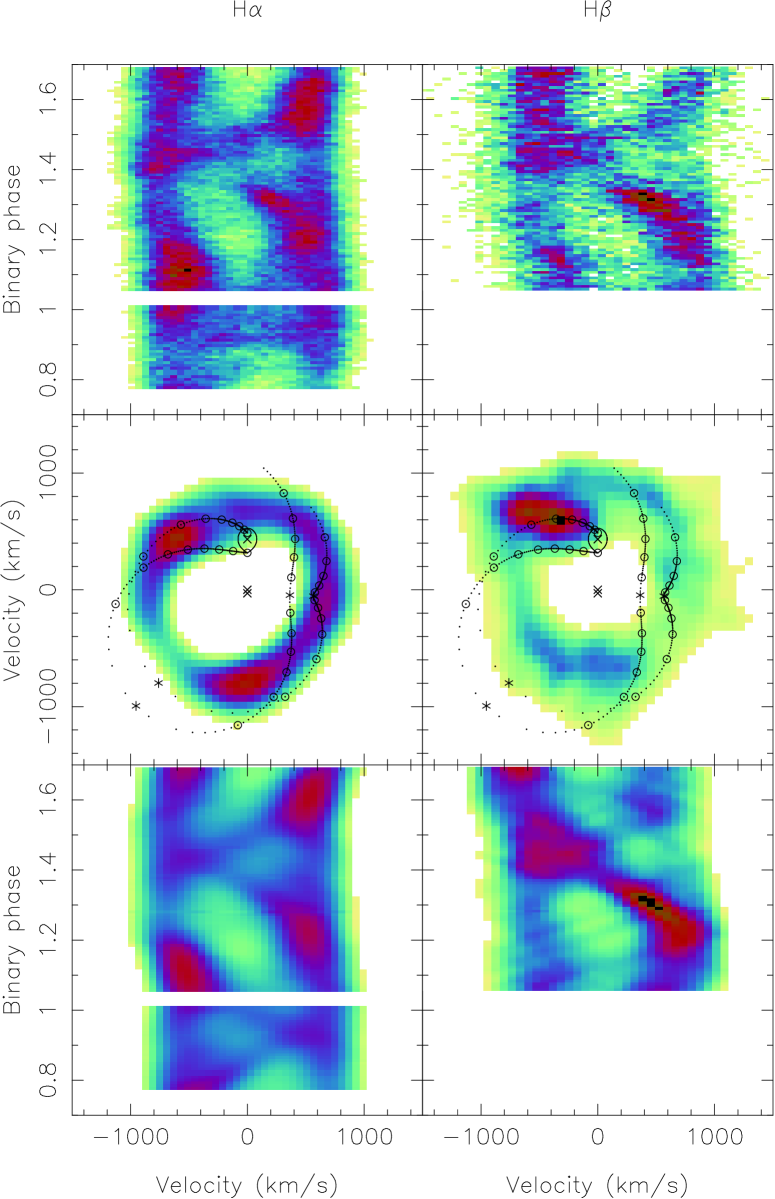
Figure 10: The Doppler images of H$\alpha$ (left panel) and H$\beta$ (right panel). From the top to bottom, the VLT data, the Doppler image and the fitted data. The “Doppler ghost” of the secondary star is shown along with the system’s centre of mass and the velocities of the compact object and secondary star (X). The two curves show the theoretical gas stream path from the inner Lagrangian point and Kepler velocity along the gas stream for $q$=0.067 and $K_{2}$=433 $\rm km\,s^{-1}$. The asterisks mark turning points in distance along the gas stream relative to the compact object. Circles have been plotted every 0.1 $R_{\rm L1}$ and dots every 0.01 $R_{\rm L1}$ along the streams.

9 Discussion

9.1 An eccentric disc?

Superhumps are optical modulations that arise when an accretion disc expands to the resonance radius, becomes elliptical and is forced to precess (Whitehurst & King, 1991). It is believed that enhanced viscous dissipation in the eccentric disc due to the tidal stress exerted by the secondary star is the source of light observed in the superhump lightcurves. Such an eccentric disc which gives rise to asymmetric emission line profiles, has been successfully used to explain the asymmetric line profiles in OY Car (Hessman et al., 1992), Z Cha (Vogt 1982, Honey et al. 1988) and AM CVn (Patterson, Halpern & Shambrook, 1993).

The Doppler maps of A0620–00 presented here show significant extended emission, strongest in H$\alpha$, with similar velocities to the stream/disc impact point, but from the opposite side of the disc between phase 0.25 and 0.50 (see Figure 10). This crescent-like structure is reminiscent of the feature seen in the Doppler maps of XTE J2123-058 in quiescence (Casares et al., 2002). Also, the orbital average H$\alpha$ profiles of XTE J1118+480 near quiescence show significant velocity variations and can be interpreted as evidence for an eccentric precessing disc (Zurita et al., 2002). Thus the most likely explanation for the crescent structure seen in the Doppler maps of A0620–00 presented here, is that it is due to an elliptical accretion disc. However, it should be noted that such structure is not seen in the Doppler maps determined by Marsh et al. (1994).

It is interesting to see what the Doppler map of an eccentric disc would look like. Smith (1999) have attempted to compute such a map and find that the Doppler map of an eccentric disc is shifted with respect to the system’s centre of mass with asymmetric enhancements in intensity around the edge of wthe disc. More recently, Foulkes et al. (2004) have performed detailed 2-D smoothed particle hydrodymanical (SPH) simulations of an eccentric precessing disc in a binary system. The synthetic trailed spectra show two distinct non-sinusoidal S-wave features which evolve with the disc precession phase which are produced by the gas stream and the disc gas at the stream-disc impact shock. These emission regions are not fixed in the co-rotating frame and vary with time over the binary orbit. To show the effects of using data that violate the assumptions inherrant in Dopper tomography, the authors produce maximum entropy Doppler maps of the SPH trailed spectra. They find that an artefact of Doppler tomography is that the stream impact emission is reconstructed in velocity space as a broad emission region between the gas stream ballistic path and the velocity of a circular Keplerian disc along the ballistic stream trajectory i.e. the stream’s “Kepler shadow” (see Figure 9 of Foulkes et al. 2004).

In both the H$\alpha$ and H$\beta$ trailed spectra of A0620–00, characteristic rapidly turning red-blue-red non-sinusoidal S-wave features between orbital phases 0.2 and 0.6 are seen, and look very similar to the simulated SPH trailed spectra of a precessing disc. The reconstructed data between phase 0.8 and 1.0 indicate that the real data are not well reproduced by sum of sinusoids that vary on the orbital period. If there is an eccentric precessing disc, as there must be if there is a superhump, the emission regions are not fixed in the co-rotating frame, it is not surprising that Doppler tomography fails. Furthermore, the broad emission near the stream/disc impact region can be interpreted as the artefact of Doppler tomography, which blurs the emission produced by the gas stream and the disc gas at the stream-disc impact region. Thus qualitatively our data suggests the presence of a precessing disc in A0620–00.

Given the mass ratio of A0620–00, the 3:1 resonance is the dominant tidal instability and lies at $R_{\rm tidal}$=0.66 $R_{\rm L1}$ . Although we derive a disc radius less than this value (see section 8.1), it should be noted that we actually determine the post-shock radius of the gas stream as it impacts the accretion disc, which most probably lies close to but not on the edge of the accretion disc. Furthermore, Foulkes et al. (2004), Hessman et al. (1992) and Rolfe, Haswell & Patterson (2001) show that the effective radius of the disc as measured by the stream-disc impact region changes dramatically with superhump phase. Thus the method of Doppler tomography will estimate a mean value for the disc’s radius. Therefore, it is possible that the radius of the accretion disc extends up to the tidal radius and so the asymmetric brightness distribution in the accretion disc we observed can be explained by the presence of a tidally distorted accretion disc.

9.2 The mechanism for the flare emission

Narayan, McClintock & Yi (1996) and Narayan, Barret & McClintock (1997) have proposed an accretion flow model to explain the observations of quiescent black hole X-ray transients. The accretion disc has two components, an inner hot advection-dominated accretion flow (ADAF) that extends from the black hole horizon to a transition radius and a thin accretion disc that extends from the transition disc to the edge of the accretion disc. Interactions between the hot inner ADAF and the cool, outer thin disc, at or near the transition radius could be a source of quasi-periodic variability. The ADAF flow requires electrons in the gas to cool via synchrotron, bremsstrahlung, and inverse Compton processes which predict the form of the spectrum from radio to hard X-rays.

It has been suggested that the flares observed in A0620–00 and other quiescent X-ray transients arise from the transition radius (Zurita et al. 2003; Shahbaz et al. 2003b). Indeed, the 0.78 mHz feature detected in V404 Cyg has been used to determine the transition radius, assuming that the periodicity represents the Keplerian period at the transition between the thin and advective disc regions (Shahbaz et al., 2003b), and a possible low frequency break in the power spectrum of A0620–00 may have a related origin (Hynes et al., 2003). In the original ADAF models the optical flux is produced by synchrotron emission. As pointed out in Shahbaz et al. (2003b), it is difficult to explain the flare spectrum in terms of optically thin synchrotron emission, unless the electrons follow a much steeper power-law electron energy distribution compared to solar flares; solar and stellar flares have a frequency spectrum with a power-law index of $\alpha$=–0.5 and an electron energy distribution with a power-law index of $\sim$–2.

However, more recently the ADAF models have been questioned, and substantial modifications proposed. Blandford & Begelman (1999) emphasised that the Bernoulli constant of the gas is positive and hence outflows are possible (as also noted by Narayan & Yi 1994). In the adiabatic inflow outflow solution (ADIOS) model of Blandford & Begelman (1999) most of the accretion energy that is released near the black hole is used to drive a wind from the surface of the accretion disc. Most of the gas that falls onto the outer edge of the accretion disc is carried by this wind away from the black hole, with the result that the hole’s accretion rate is much smaller than the disc’s accretion rate. Advective flows are also expected to be convectively unstable, as also remarked by Narayan & Yi (1994). In these models the central accretion rate can also be suppressed. For either of these cases, the effect is to shift the source of cooling outwards, and the optical synchrotron emission is reduced (Quataert & Narayan 1999; Ball, Narayan, & Quataert 2001). In these more realistic cases $optical$ flares directly from the inner flow are less likely. Optical emission might still arise from the inner edge of the outer (thin) disc, or from reprocessing of X-ray variability.

9.3 Do the flares arise from the whole disc?

It was argued by Hynes et al. (2002) that since large ($\sim$ few d) flares in V404 Cyg involve enhancements of both blue and red wings of H$\alpha$, they must involve the whole disc. While these observations indicate participation by a wide range of azimuths, they leave open the possibility that only the inner disc is involved. Using simultaneous multicolour photometry Shahbaz et al. (2003b) determined the colour of similar large flares in V404 Cyg. Although the flare parameters determined are complicated by uncertainties in the interstellar reddening, the flare temperature was estimated to be $\sim$8000 K. Flares on timescales similar to those present in A0620–00 (i.e. tens of minutes) were also observed, but no physical parameters could be determined given the large uncertainties in the colour. The large ($\sim$ few hrs) flares were observed to arise from regions that cover at least 3 percent of the disc’s surface area. Shahbaz et al. (2003b) have suggested that the large ($\sim$ few hrs) flares in V404 Cyg are produced in regions further out or further above the disc from a corona than the rapid ($\sim$0.5 hr) and more rapid ($\sim$ min) flares.

If the flares in V404 Cyg and A0620–00 have the same origin, then it is interesting to note that the large flares ($\sim$ few hrs) observed in V404 Cyg cover a larger surface area of the disc compared to the rapid (tens of mins) flares observed in A0620–00, which is consistent with the idea that the large flares arise from regions that extend further out into the disc compared to the rapid flares. Although the flare temperatures derived suggest that large flares are cooler than rapid flares, the uncertainties are large and so no meaningful conclusion can be drawn at this stage. Accurate physical parameters for the flares can only be obtained by resolving the Balmer jump and Paschen continuum.

9.4 Do the flares arise from the bright-spot?

For the data presented here on A0620–00, there is evidence that some of the flare events in the continuum lightcurve are correlated with the Balmer emission line lightcurves, similar to what is observed in V404 Cyg (Hynes et al., 2002). The value for the Balmer decrement suggests that the persistent flux is optically thin and the decrease of the Balmer decrement during the flares suggests a significant temperature increase. We find that the optically thin spectrum of the flare, which lasts tens of minutes, has a temperature of $\sim$12000 K and covers 0.08 percent of the disc’s projected surface area (see section 7).

In many high inclination systems the continuum light from the bright-spot produces a single hump in the lightcurve, because the bright-spot is obscured by the disc when it is on the side of the disc facing away from the observer. Since A0620–00 is at an intermediate inclination angle (41^∘; Shahbaz et al. 1994 and Gelino et al. 2001) where no strong obscuration effects are predicted, it is not surprising that the continuum lightcurve does not show obvious evidence of a bright-spot. From the Doppler maps of A0620–00 (see section 8.1), it is clear that the bright-spot is present in the Balmer emission lines. If the bright spot were present in the continuum then we would expect strong correlations between the continuum and emission line lightcurves. Indeed we see some evidence for such correlations in the lightcurves (see Figures 2 and 5). It is interesting to note that the flare temperature and area we obtain (see section 7) is consistent with the bright-spot temperature and radius determined by Gelino et al. (2001). Therefore, with the data presented here we cannot rule out the possibility that the flares arise from the bright-spot. Although, this hypothesis can only be tested by observing high inclination X-ray transients, where one would expect the orbital distribution of the flares and lightcurves to be indicative, it should be noted that the kinematics of the flares in V404 Cyg do rule out at least some of the flares coming from the bright spot.

10 CONCLUSION

We have presented a time-resolved spectrophotometric quiescent study of the optical variability in A0620–00. We observe the well known flare events which and find that some of the events appear in both the continuum and the emission line lightcurves. The Balmer line flux and variations suggest that that the persistent emission is optically thin and the drop in the Balmer decrement for the flare event at phase 1.15, suggests that either a significant increase in temperature occurred during the flare or that the flare is more optically thick than the continuum. The data suggests that there are two HI emitting regions, the accretion disc and the accretion stream/disc region, with different Balmer decrements. The orbital modulation of H$\alpha$ with the continuum suggests that the steeper decrement is most likely associated with the stream/disc impact region.

We find that flare spectrum can be described by an optically thin gas with a temperature in the range 10000–14000 K that covers 0.05–0.08 percent (90 percent confidence) of the accretion disc’s surface. Given these parameters, the possibility that the flares arise from the bright-spot cannot be ruled out.

Finally, Doppler images of the H$\alpha$ and H$\beta$ emission show enhanced emission at the stream/disc impacts region as well as extended structure from the opposite side of the disc. The trailed spectra show characteristic S-wave features that can be interpreted in the context of an eccentric accretion disc.

References

- Avni & Bahcall (1975) Avni Y., Bahcall, J. N., 1975, ApJ, 197, 675
- Ball, Narayan, & Quataert (2001) Ball G. H., Narayan R., Quataert E., 2001, ApJ, 552, 221
- Blandford & Begelman (1999) Blandford R. D., Begelman M. C, 1999, MNRAS, 303, L1
- Boley & Wolfson (1976) Boley F., Wolfson R., 1975, IAU Circ. 2819
- Casares et al. (2002) Casares J., Dubus G., Shahbaz T., Zurita C., Charles P. A., 2002, MNRAS, 329, 29
- Elvis et al. (1975) Elvis M., Grifiths C. G., Turner M. J. L., Page C., 1975, IAU Circ. 2184
- Froning & Robinson (2001) Froning C. S., Robinson E. L., 2001, AJ, 121, 2212
- Foulkes et al. (2004) Foulkes S. B., Haswell C. A., Murray J. R., Rolfe D. J., 2004, MNRAS, 349, 1179
- Gelino et al. (2001) Gelino D. M., Harrison T. E., Orosz J. E., 2001, AJ, 122, 2668
- Gunn & Stryker (1983) Gunn J. E., Stryker L. L., 1983, ApJS, 52, 121
- Haswell (1992) Haswell C. A., 1992, Ph.D thesis, University of Texas.
- Haswell et al. (1993) Haswell C. A., Robinson E. L., Horne K., Stiening, R. F., Abbott T. M. C., 1993, ApJ, 411, 802
- Haswell (1996) Haswell C.A., 1996, in Compact stars in binaries, IAU symposium 165, 351
- Hessman et al. (1992) Hessman F. V., Mantel K., Barwig H., Schoembs R, 1992, A&A, 263, 147
- Honey et al. (1988) Honey W. B., Charles P. A., Whitehurst R., Barrett P. B., Smale A. P., 1988, MNRAS, 231, 1
- Horne (1986) Horne K., 1986, PASP, 98, 609
- Hynes et al. (2002) Hynes R. I., Zurita C., Haswell C. A., Casares J., Charles P. A., Pavlenko E. P., Shugarov S. Yu., Lott D. A., 2002, MNRAS, 330, 1009
- Hynes et al. (2003) Hynes R. I., Charles P. A., Casares J., Haswell C. A., Zurita C., Shahbaz T., 2003, MNRAS, 340, 447
- Khruzina & Cherepashchuk (1995) Khruzina T. S., Cherepashchuk A. M., 1995, ARep, 39, 178
- Leibowitz Hemar & Orio (1998) Leibowitz E. M., Hemar S., Orio M., 1998, MNRAS, 300, 463
- McClintock et al. (1983) McClintock J. E., Petro I. D., Remillard R., Ricker G. R., 1983, ApJ, 266, L27
- McClintock et al. (1995) McClintock J. E., Horne K., Remillard R., 1995, ApJ, 442, 358
- McClintock & Remillard (2000) McClintock J. E., Remillard R., 2000, ApJ, 531, 956
- Marsh & Horne (1988) Marsh T.R., Horne K., 1988, MNRAS, 235, 26
- Marsh et al. (1990) Marsh T. R., Horne K., Schlegel E. M., Honeycutt R. K., Kaitchuck R. H., 1990, ApJ, 364, 637
- Marsh et al. (1994) Marsh T. R., Robinson E.vL, Wood J. H., 1994, MNRAS, 266, 137
- Narayan & Yi (1994) Narayan R., Yi I., 1994, ApJ, 428, L13
- Narayan, Barret & McClintock (1997) Narayan R., Barret D., McClintock J. E., 1997, ApJ, 482, 448