SHAPES AND ALIGNMENTS OF GALAXY CLUSTER HALOS
         

Abstract

We present distribution functions and spatial correlations of the shapes of dark matter halos derived from Hubble Volume simulations of a $\Lambda$CDM  universe. We measure both position and velocity shapes within spheres encompassing mean density 200 times the critical value, and calibrate small-N systematic errors using Poisson realizations of isothermal spheres and higher resolution simulations. For halos more massive than $3\times 10^{14}\hbox{$\,h^{-1}$}{\rm M}_{\odot}$, the shape distribution function peaks at (minor/major, intermediate/major) axial ratios of $(0.64,0.76)$ in position, and is rounder in velocity, peaking at $(0.72,0.82)$. Halo shapes are rounder at lower mass and/or redshift; the mean minor axis ratio in position follows $\langle c/a\rangle(M,z)=c_{15,0}[1-\alpha\ln(M/10^{15}\hbox{$\,h^{-1}$}{\rm M}_{\odot})](1+z)^{-\varepsilon}$, with $c_{15,0}\!=\!0.631\pm 0.001$, $\alpha\!=\!0.023\pm 0.002$ and $\varepsilon\!=\!0.086\pm 0.004$. Position and velocity principal axes are well aligned in direction, with median alignment angle $22^{\circ}$, and the axial ratios in these spaces are correlated in magnitude. We investigate mark correlations of halo pair orientations using two measures: a simple scalar product shows $\geq 1\%$ alignment extending to $30\hbox{$\,h^{-1}$}{\rm\ Mpc}$ while a filamentary statistic exhibits non-random alignment extending to scales $\sim\!200\hbox{$\,h^{-1}$}{\rm\ Mpc}$, ten times the sample two-point correlation length and well into the regime of negative two-point correlation. Cluster shapes are unaffected by the large-scale environment; the shape distribution of supercluster members is consistent with that of the general population.

1. INTRODUCTION

Clusters of galaxies signal the largest gravitationally bound dark matter halos in the universe. They are mildly aspherical systems that tend to be aligned by mergers directed by interconnecting filaments in the cosmic web.

Since the early days of extragalactic astronomy, it has been apparent that clusters are generally elongated on the sky. Flattening of these clusters due to rotation was ruled out Illingworth (1977) and many assumed that the flattening was due to gravitational instabilities expected in the top-down scenario of Zel’dovich (1978) and Doroshkevich et al. (1978). The groundbreaking work of Carter and Metcalfe (1980) showed that the aspherical shape of a cluster was connected with the velocity anisotropy of the orbits of cluster galaxies. Binney and Silk (1979) proposed that this anisotropy was due to tidal distortion from neighboring large-scale structure.

Binggeli (1982) was the first to investigate alignments of close cluster pairs. He studied 44 Abell clusters and found that galaxies separated by less than 30 Mpc show a strong alignment with each other and that the orientation of a cluster was dependent on the distribution of surrounding clusters. Other observational claims of cluster alignments have been made, both with nearest neighbors and with other clusters in the same supercluster West 1989a ; West 1989b ; Rhee et al. (1992); Richstone et al. (1992); Plionis (1994).

With some exceptions (for example, Struble and Peebles (1985) or Rhee and Katgert (1987)), most work in the literature de Theije et al. (1995); West et al. (1995); West 1989a ; Rhee et al. (1992); Onuora & Thomas (2000) confirms Binggeli’s original results. West (1989a) uses 48 Abell superclusters and finds a tendency for clusters within $60\hbox{$\,h^{-1}$}{\rm\ Mpc}$ to be aligned. Plionis (1994) measures alignments for 637 Lick clusters and finds strong alignments up to $15\hbox{$\,h^{-1}$}{\rm\ Mpc}$ with weaker alignments out to $60\hbox{$\,h^{-1}$}{\rm\ Mpc}$. West et al. (1995) finds a marked anisotropy for Einstein clusters extending out to $10\hbox{$\,h^{-1}$}{\rm\ Mpc}$.

Simulations have shown that spatial alignments, intrinsically predicted from the ’top-down’ model Zel’dovich (1970), are also seen in bottom-up (cold dark matter) scenarios, where halos form by mergers of smaller structures organized along filaments Struble & Ftaclas (1994); West et al. (1991, 1995). Simulations also show that the orientation of the major axis of a galaxy cluster is aligned with the direction of the last major merger event van Haarlem & van de Weygaert (1993); Splinter et al. (1997). Since cluster alignments appear to be a generic outcome of gravitational instability, their use as a discriminant of cosmological models requires careful calibration Onuora & Thomas (2000).

In the halo model description of non-linear structure (Cooray and Sheth 2002), all matter is contained in bounded, spatially correlated regions (the halo population) that span a spectrum of sizes. Most instances of this model assume spherically symmetric halos, but more precise versions will need to take into account the spectrum of halo shapes, including detailed internal structure (Jing & Suto 2002), as well the spatial correlation of the shapes of neighboring halos (Jing 2002; Faltenbacher et al. 2003).

In this paper, we report measurements of shape statistics, including spatial (or mark) correlations of alignments, derived from large samples of massive dark matter halos extracted from Hubble Volume simulations. We investigate two flat-metric cosmologies ($\Lambda$CDM and $\tau$CDM) dominated by vacuum energy and dark matter, respectively. We focus on the former, more empirically satisfying model, but show results for the latter for comparative purposes. Section 2 provides details of the simulations and describes our method of finding principal axis orientations and magnitudes for mass-limited halo samples. In § 3, we use Poisson realizations of isothermal spheres to estimate systematic error in mean shape measurement due to shot noise. We then present axial ratio distribution functions for mass-limited samples, and characterize the dependence of halo shape on mass and redshift. Section 4 presents mark correlations of $\Lambda$CDM cluster alignments and briefly examines the role of supercluster membership on shape. A final section reviews our conclusions.

Unless explicitly stated otherwise, the halo mass $M$ used throughout this paper is a critically-thresholded, spherical overdensity mass ($M_{200}$) expressed in units of $10^{15}\hbox{$\,h^{-1}$}{\rm M}_{\odot}$, with $h\!=\!{\rm\ H_{o}}/100{\rm km\ s^{-1}\ Mpc^{-1}}$.

2. CLUSTER SHAPES FROM SIMULATIONS

We use two sets of simulations to investigate dark matter halo shapes. The large Hubble Volume (HV) simulations provide statistical power but poor mass resolution, while higher resolution, but smaller volume, Virgo simulations are used for resolution tests.

2.1. Simulations

The HV simulations are a pair of gigaparticle N-body simulations created using a parallel version of the Hydra N-body code Macfarland et al. (1998). Random realizations of two cosmologies with flat spatial metric are produced: a $\Lambda$CDM  model with $\Omega_{m}=0.3$, $\Omega_{\Lambda}=0.7$ and power spectrum normalization $\sigma_{8}=0.9$ and a $\tau$CDM model with $\Omega_{m}=1$, $\Omega_{\Lambda}=0$, and $\sigma_{8}=0.6$. The dark matter structure is resolved by particles of mass $2.2\times 10^{12}\hbox{$\,h^{-1}$}{\rm M}_{\odot}$ within periodic cubic volumes of length 3000 and $2000\hbox{$\,h^{-1}$}{\rm\ Mpc}$, respectively (see Table 1). We analyze $z\!=\!0$ and combined sky survey samples of galaxy cluster halos published in Evrard et al.  (2002). The reader is referred to that paper for details of the simulations, including the process of sky survey creation.

Table 1Model Parameters

Model	$\Omega_{m}$	$\Omega_{\Lambda}$	$\sigma_{8}$	$z_{init}$	$L$	$m$
$\Lambda$CDM	0.3	0.7	0.9	35	3000	$2.25$
$\tau$CDM	1.0	0.0	0.6	29	2000	$2.22$

For resolution tests, we employ the $256^{3}$–particle Virgo simulations of Jenkins et al. (1998). These simulations have order-of-magnitude improved mass resolution but much smaller samples than the HV simulations.

2.2. Halo Finding Algorithm

We define dark matter halos with a spherical overdensity (SO) group finder that identifies as a halo the set of particles lying within a sphere of size $r_{200}$, centered on a particle that represents a local density maximum filtered on a scale of $2\times 10^{13}\hbox{$\,h^{-1}$}{\rm M}_{\odot}$. The size measure $r_{200}$ is the radius of the sphere within which the mean density is 200$\rho_{c}(z)$, with $\rho_{c}(z)$ the critical density at redshift $z$. The total mass $M_{200}$ lying within r₂₀₀ is the basic order parameter of the halo sample. As a result of ongoing merging activity, roughly $7.5\%$ of halos are found to have overlapping $r_{200}$ spheres. We retain both members of an overlapping pair in the halo sample.

2.3. Sky Surveys

In addition to the traditional mode of fixed proper-time output, sky survey samples, consisting of data collected along the past light cone of hypothetical observers located within the computational volume, were also generated by the HV simulations. We use two octant surveys (PO and NO) that cover $\pi/2$ sterad and extend to $z_{max}\!=\!1.46$ for $\Lambda$CDM  and 1.25 for $\tau$CDM, as well as two full-sky surveys (MS and VS) that reach $z_{max}\!=\!0.57$ for $\Lambda$CDM  and 0.42 for $\tau$CDM. The octants sample structure over the last $74\%$ ($\Lambda$CDM) and $71\%$ ($\tau$CDM) of the age of the universe, approximately a 10 Gyr look-back time. Halos in these surveys are defined using the SO method described above.

2.4. Cluster Shapes

Given the modest resolution of the HV data, we take a simple approach and estimate the shape of a halo using the moments of the material within $r_{200}$.

With respect to the center of the halo (defined by the local gravitational potential minimum), we compute the $3\times 3$ symmetric tensor $M_{jk}$

$$M_{jk}\ =\ \frac{1}{N_{h}}\ \sum_{\alpha}x_{\alpha j}x_{\alpha k}$$ (1)

where $x_{\alpha j}$ is the j^th component of the displacement vector of particle $\alpha$ relative to the halo center and $N_{h}$ is the number of (equal mass) particles in the halo. We diagonalize to find eigenvalues $\lambda_{j}$ and unit eigenvectors. The sorted eigenvalues ($\lambda_{1}>\lambda_{2}>\lambda_{3}$) and vectors define principle axes $a,b,c$, with semi-major axis $a=\sqrt{\lambda_{1}}$, intermediate $b\!=\!\sqrt{\lambda_{2}}$, and $c\!=\!\sqrt{\lambda_{3}}$ of a triaxial ellipsoid that approximates the halo. We refer to the corresponding unit vector directions as $\hat{a}$, $\hat{b}$ and $\hat{c}$.

Velocity moments are solved for in a similar way, using a mean defined as the center of mass velocity of the material within $r_{200}$. For compactness of notation, we define intermediate and minor axial ratios as follows

$$\tilde{b}\ \equiv\ b/a,$$ (2)

$$\tilde{c}\ \equiv\ c/a.$$ (3)

We have confirmed that the halo population is oriented randomly with respect to the Cartesian coordinates of the simulation, as required by the cosmological principal.

3. HALO SHAPE STATISTICS

We begin this section by estimating the error on shape determinations due to shot noise. From Monte Carlo realizations of distorted isothermal spheres, we find that population mean values of $\tilde{c}$ and $\tilde{b}$ are accurate to a few percent if $N_{h}\gtrsim 100$. We then present the joint distribution function $p(\tilde{c},\tilde{b})$ at $z\!=\!0$, and investigate joint position and velocity shape statistics. We follow with the mass and redshift dependence of the minor axis ratio.

3.1. Resolution Tests

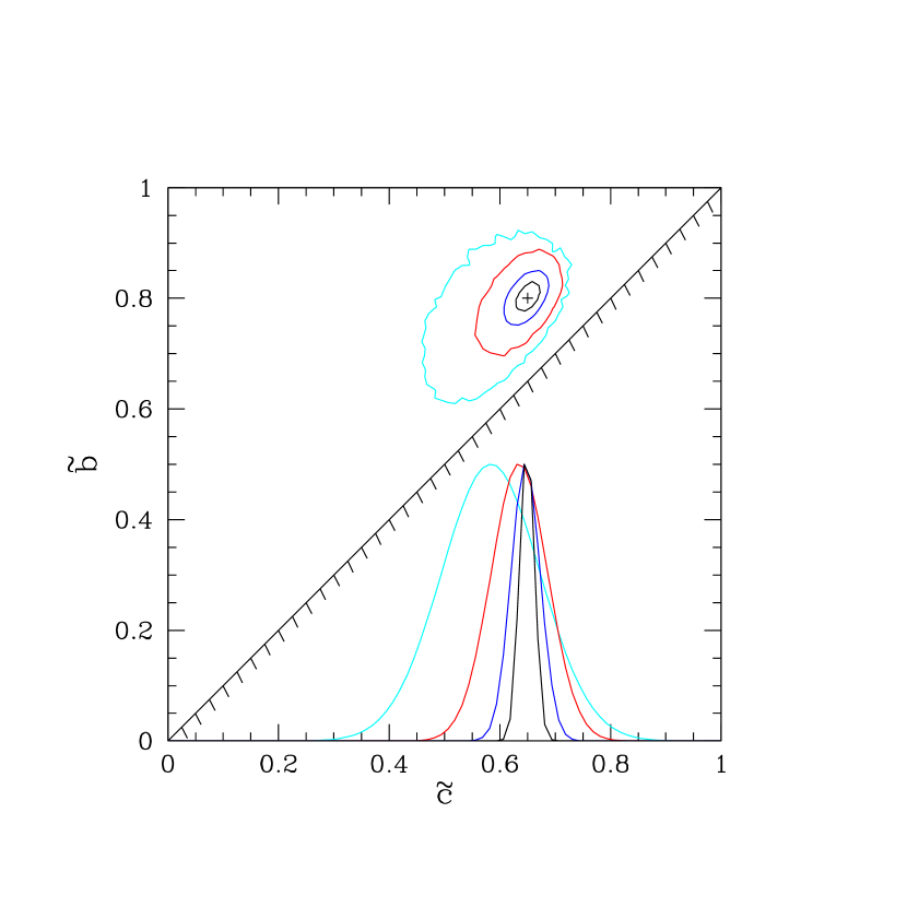
Figure 1.— Estimates of the effect of Poisson noise on measurement of minor ($\tilde{c}$) and intermediate ($\tilde{b}$) axis ratios. Halos must lie in the upper left portion of the plot, with spherical objects at $(1,1)$, oblate halos tending to $\tilde{b}\!=\!1$ and prolate halos lying near the diagonal $\tilde{b}\!=\!\tilde{c}$. Contours show $68\%$ confidence regions of axial ratios measured from 10,000 random realizations of isothermal spheres distorted to mean shape $(0.65,0.80)$, shown by the cross, and resolved by (from outer to inner contours) 40, 160, 640, and 2560 particles. Histograms in the lower right give frequency distributions of the minor axis ratio $\tilde{c}$. As resolution degrades, the mean is biased to lower values and the dispersion grows.

To calibrate the error in mean shape due to the small numbers of particles used to resolve clusters in the HV, we carry out the following resolution test. Halo models are created using a set of $N_{h}$ particles with an initially spherical, isothermal profile. To simulate the mean ellipticity of the HV cluster samples discussed below, each cluster is then compressed along the $(x,y)$-axes by fixed amounts (0.65, 0.8). The particle moments are calculated and used to estimate the shape of each cluster in the same manner as for the HV clusters (see section 2.4). Generating ensembles at several values of $N_{h}$, we calibrate the bias in mean cluster shape as a function of mass resolution.

The results for an ensemble of 10,000 clusters at each $N_{h}$ are presented in Figure 1. Mean axial ratio values $\langle\tilde{c}\rangle$ and $\langle\tilde{b}\rangle$ are presented in Table 2 for $N_{h}$ ranging from 40 to 2560 particles. In Figure 1, the measured shape distribution function has a dispersion ranging from 0.09 at $N_{h}$=40 to 0.01 at $N_{h}$=2560, and the mean is offset from the input values by a bias that scales inversely with particle number $0.024(N_{h}/100)^{-1}$. We will use this calibration to bias-correct the mass-dependent shapes presented in § 3.4.

Table 2Resolution Test Values

$N_{h}$	$\langle\tilde{c}\rangle$	$\sigma_{\tilde{c}}$	$\langle\tilde{b}\rangle$	$\sigma_{\tilde{b}}$
40	0.584	0.089	0.777	0.095
160	0.635	0.051	0.794	0.061
640	0.647	0.026	0.799	0.032
2560	0.649	0.013	0.799	0.016

3.2. Shape Distributions

To ensure a mean shape measurement biased by less than two percent, we impose a mass limit $\hbox{$M_{200}$}\geq 3\times 10^{14}\hbox{$\,h^{-1}$}{\rm M}_{\odot}$, corresponding to 133 particles in the HV simulations. We note that Jing (2002) also finds that 160 particles are sufficient for percent-level shape measurement. To keep the corrections small while maintaining a moderate sample size, the Virgo data are cut at a mass of $10^{14}\hbox{$\,h^{-1}$}{\rm M}_{\odot}$, equivalent to 1467 particles for the $\Lambda$CDM case and 440 particles for the $\tau$CDM case. The numbers of halos in each sample are listed in Table 3.

Table 3Halo Samples at $z\!=\!0$

Model	$M_{min}[\hbox{$\,h^{-1}$}{\rm M}_{\odot}]$	Ncl
$\Lambda$CDM$-$HV	$3\times 10^{14}$	82967
$\Lambda$CDM$-$Virgo	$10^{14}$	353
$\tau$CDM$-$HV	$3\times 10^{14}$	87121
$\tau$CDM$-$Virgo	$10^{14}$	703

The distribution of axial ratios at $z\!=\!0$ for 82,967 ($\Lambda$CDM) and 87,121 ($\tau$CDM) halos are given in Figure 2. The top row shows the distributions in position space while the bottom row shows velocity space. The location of the mean axial ratios ($\langle\tilde{c}\rangle$, $\langle\tilde{b}\rangle$) is depicted by a cross for HV and an asterisk for Virgo data.

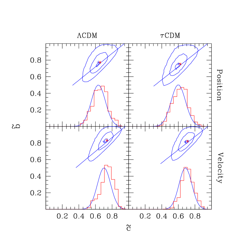
Figure 2.— Contours of the joint probability distribution of axial ratios $p(\tilde{c},\tilde{b})$ are shown with the minor-axis frequency distribution $p(\tilde{c})$ in the same format as Figure 1. Left and right columns show the $\Lambda$CDM  and $\tau$CDM models while upper and lower rows give position and velocity space distributions. Contour levels in the joint pdf are drawn at the 10th, 50th, and 95th percentiles of the enclosed distribution. Gaussian fits to the frequency distribution of $\tilde{c}$ are shown for the HV simulations while histograms show $\tilde{c}$ values derived from the Virgo simulations. Crosses and asterisks mark the locations $(\langle\tilde{c}\rangle,\langle\tilde{b}\rangle)$ of the mean shapes for the HV and Virgo models, respectively.

Consistent with previous studies, we find galaxy cluster halos to be mostly prolate in shape, and somewhat rounder in velocity compared to position space. Table 4 summarizes the $z\!=\!0$ shape data. The $\Lambda$CDM  HV simulation has modal values ($\tilde{c}$,$\tilde{b}$)${}_{peak}^{P}=(0.64,0.76)$ and ($\tilde{c}$,$\tilde{b}$)${}_{peak}^{V}=(0.72,0.82)$ in position and velocity, while the $\tau$CDM model halos are more strongly ellipsoidal, with values ($\tilde{c}$,$\tilde{b}$)${}_{peak}^{P}=(0.59,0.72)$ and ($\tilde{c}$,$\tilde{b}$)${}_{peak}^{V}=(0.70,0.80)$.

The frequency distribution of minor axis ratio $\tilde{c}$, computed by integrating the joint pdf along the $\tilde{b}$ axis, is well fit by a Gaussian for the HV samples. Distributions of $\tilde{c}$ derived from the Virgo simulations, shown as histograms in Figure 2, are generally in good agreement with the HV data. The distribution of $\Lambda$CDM minor axis ratios for position is centered on $0.635$ and has measured dispersion $0.086$. When corrected for Poisson error, the estimated mean is slightly larger $\langle\tilde{c}\rangle\!=\!0.647$ and the intrinsic dispersion is estimated to be $0.076$. While the statistical uncertainty in the mean is in the third significant digit, the level of systematic uncertainty is certainly larger.

Table 4Mean Halo Shapes at $z\!=\!0$

Model-Space	$(\tilde{c},\tilde{b})_{peak}$	$\langle\tilde{c}\rangle$	$\sigma_{\tilde{c}}$	$\langle\tilde{b}\rangle$	$\sigma_{\tilde{b}}$
$\Lambda$CDM$-$P	(0.635, 0.760)	0.635	0.086	0.776	0.096
$\Lambda$CDM$-$V	(0.719, 0.823)	0.704	0.080	0.818	0.088
$\tau$CDM$-$P	(0.593, 0.719)	0.600	0.087	0.754	0.102
$\tau$CDM$-$V	(0.698, 0.802)	0.686	0.077	0.814	0.086

A crude estimate of systematic error is given by the $0.012$ Poisson bias correction for the mass-limited sample. However, at the level of $0.01$, a number of other effects on axial ratio come into play. Foremost among them is the detailed definition of a halo: its location, scale, and geometry. We use the common spherical overdensity (SO) definition of halos as spherical regions centered on local density peaks. Other viable approaches, such as friends-of-friends grouping or use of an ellipsoidal boundary can systematically shift shape measurements by many percent (Warren et al. 1992, Jing & Suto 2002). We leave it to future work to address such systematic effects in detail.

The finding that halos are rounder in velocity space may be at least partly due the effects of ongoing mergers. Mergers will scatter in velocity space first, followed by mixing and relaxation of particle positions. Another factor pushing in the same direction is that the gravitational potential that drives the velocity field is rounder than the density distribution.

We do not attempt to formally fit the joint probability distribution $p(\tilde{c},\tilde{b})$, as doing so would requite a full deconvolution of the effects of shot noise. However, to give an indication of the joint pdf shape, we locate the peak in the intermediate axis conditional probability

$$p(\tilde{b}|\tilde{c})\ =\ \frac{p(\tilde{c},\tilde{b})}{p(\tilde{c})}$$ (4)

and record the modal intermediate axis ratio $\tilde{b}_{mod}$ as a function of minor axis ratio $\tilde{c}$. The lines in each panel of Figure 2 show fits $\tilde{b}_{mod}(\tilde{c})\!=\!r\tilde{c}+s$, with fit parameters given in Table 5.

Table 5Intermediate Axis Modal Ridge Line $\tilde{b}_{mod}(\tilde{c})$

Model	Component	$r$	$s$
$\Lambda$CDM	Position	$0.81\pm 0.02$	$0.24\pm 0.01$
	Velocity	$0.84\pm 0.03$	$0.20\pm 0.02$
$\tau$CDM	Position	$0.79\pm 0.02$	$0.25\pm 0.01$
	Velocity	$0.79\pm 0.03$	$0.25\pm 0.02$

3.3. Position-Velocity Major Axis Alignment

Since elongated orbits drive both position and velocity anisotropy, a correlation between both position and velocity major axes is both expected and measured in simulations (Tormen 1997). We quantify the alignment between position and velocity in a halo through the scalar product of its major axis eigenvectors

$$\cos(\theta_{PV})\ =\ |\hat{a}^{P}\cdot\hat{a}^{V}|.$$ (5)

Figure 3 shows cumulative probability functions of this statistic for the $\Lambda$CDM HV and Virgo models.

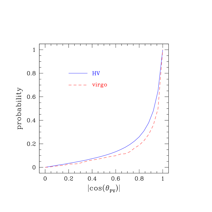
Figure 3.— Cumulative distributions of the alignment angle between the position and velocity major axes are shown for the $\Lambda$CDM  HV clusters with $\hbox{$M_{200}$}\geq 3\times 10^{14}\hbox{$\,h^{-1}$}{\rm M}_{\odot}$ (solid line) and $\Lambda$CDM  Virgo clusters with $\hbox{$M_{200}$}\geq 10^{14}\hbox{$\,h^{-1}$}{\rm M}_{\odot}$ (dashed line). Half of the clusters in the $\Lambda$CDM HV simulations have an alignment angle smaller than 22 degrees.

We find a strong alignment signal: half of all halos have position and velocity major axes aligned to better than 22 degrees for the HV $\Lambda$CDM model (21 degrees for $\tau$CDM). The higher resolution Virgo runs show even stronger position-velocity alignment, with median values of 15 degrees for $\Lambda$CDM and 14 degrees for the $\tau$CDM simulation. When the same analysis is carried out using only strongly ellipsoidal clusters ($\tilde{c}<0.635$), the results do not significantly change.

Our results are consistent with a higher resolution study of Tormen (1997), who finds from simulations of 9 dark matter halos resolved by 20,000 particles that the position-velocity alignment angle is approximately 30 degrees.

To further define the relationship between position and velocity space, we show the joint distribution of minor axis ratios $(\tilde{c}^{P},\tilde{c}^{V})$ in Figure 4. The likelihood is well fit by a Gaussian in an ellipsoidal coordinate $r$, where $r^{2}=(\frac{c_{+}}{\sigma_{+}})^{2}+(\frac{c_{-}}{\sigma_{-}})^{2}$ and $c_{\pm}=\frac{1}{\sqrt{2}}[(\tilde{c}^{P}-\langle\tilde{c}^{P}\rangle)\pm(\tilde{c}^{V}-\langle\tilde{c}^{V}\rangle)]$ are principal component directions centered on the one-component means of the distribution. This fit is shown by the dotted lines in Figure 4. The measured dispersions for $\Lambda$CDM are $\sigma_{+}\!=\!0.096$ and $\sigma_{-}\!=\!0.069$. The bold contour shows the median of the enclosed distribution.

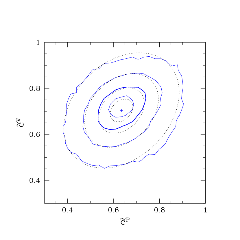
Figure 4.— Joint probability density of the position $\tilde{c}^{P}$ and velocity $\tilde{c}^{V}$ minor axis ratios. Light contours show the 16th, 50th, 84th and 99th percentiles of the enclosed distribution while dotted contours show the same for the ellipsoidal Gaussian fit described in the text. The bold contour highlights the median of the joint distribution.

Since essentially all cluster detection methods use some power of projected mass density as a defining signal, the spatial-velocity alignments examined here will introduce an orientation bias in estimates of velocity dispersions for clusters lying close to the sample detection threshold. The magnitude of this effect will depend on the specific sample in question, but the general trend will be for the line-of-sight dispersion to overestimate its isotropic counterpart, by a fractional amount that could be $\sim\!10\%$ for small samples of moderate signal-to-noise detections. Estimating the effect for particular observational surveys is best done using Monte Carlo sample realizations, such as those performed for the 2MASS (Kochanek et al. 2003) and SDSS (Miller et al. 2004; Wechsler et al. 2004) samples.

3.4. Mass and Redshift Dependence

Because mergers are directed along large-scale filaments in the cosmic web, the birth of dark matter halos is an inherently asymmetric process. As a merger evolves, dynamical relaxation will tend to drive a halo closer to isotropy. One then expects that dynamically younger clusters will be more strongly ellipsoidal than older ones. Equating dynamical age with elapsed time from a halo’s formation epoch (defined, for example, using the mass accretion history by Wechsler et al. 2002), we expect high mass halos at a given epoch will be more elongated than those of lower mass. Similarly, at fixed mass, high-z halos should be more ellipsoidal than their low-z counterparts of the same mass.

With the large number of clusters in the $z\!=\!0$ sample, we first investigate the mass dependence at the present epoch. Figure 5 shows the dependence of mean minor axis ratio shapes in position (filled symbols) and velocity (open symbols) on halo mass, using bins of width 0.1dex. Error bars on the points give the uncertainty in the mean. Circles show the HV data while squares show the Virgo data. Small symbols show the raw mean shape measurements while large symbols correct for the bias in mean shape calibrated in section 3.1. There is generally good agreement between the bias-corrected mean shapes of the HV models and the values measured directly from the higher resolution Virgo runs.

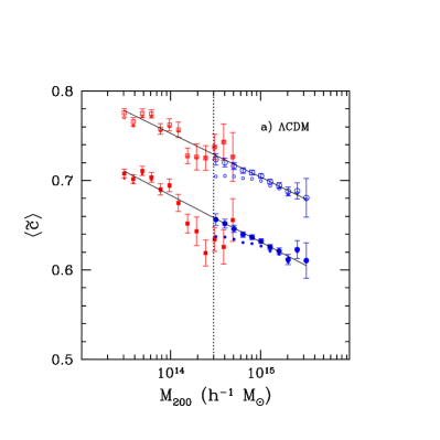
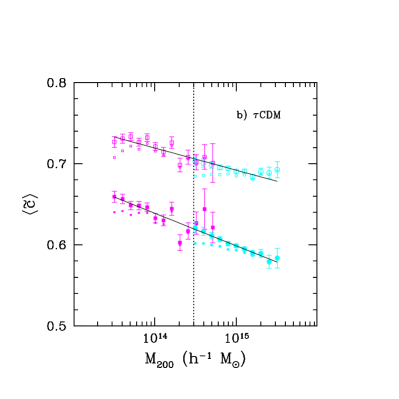
Figure 5.— The dependence of mean minor axis ratio on mass is shown for halo samples at z=0 of the a) $\Lambda$CDM  and b) $\tau$CDM models. The upper curve with open symbols give velocity shapes while the lower curve with filled symbols show position. Small symbols show measures uncorrected for small-N effects while bigger symbols have Poisson corrections applied, as discussed in the text. Circles and squares are HV and Virgo model results, respectively, and the vertical dotted line marks the $3\times 10^{14}\hbox{$\,h^{-1}$}{\rm M}_{\odot}$ resolution limit of the HV models. Solid lines show the weak logarithmic dependence on mass, equation (8), with parameter values given in Table 6. Higher mass clusters are more strongly ellipsoidal than low mass clusters in both position and velocity.

The mass dependence favors more ellipsoidal halos at higher mass. The mean minor axis ratios of both the position and velocity shapes vary by only $\sim\!5$ percent as the mass changes by a factor of ten. For the $\Lambda$CDM model, a fit to a logarithmic mass dependence using HV data above $3\times 10^{14}\hbox{$\,h^{-1}$}{\rm M}_{\odot}$ and Virgo data below yields

$$\langle\tilde{c}^{P}\rangle\ =\ (0.631\pm 0.001)\ \bigl{(}1-(0.023\pm 0.002)\ln M\bigr{)},$$ (6)

$$\langle\tilde{c}^{V}\rangle\ =\ (0.704\pm 0.001)\ \bigl{(}1-(0.021\pm 0.001)\ln M\bigr{)}$$ (7)

where $M$ is the halo mass measure $M_{200}$ expressed in units of $10^{15}\hbox{$\,h^{-1}$}{\rm M}_{\odot}$. Although these expressions are good fits to the shape dependence over two orders of magnitude in mass, the limit $\tilde{c}\leq 1$ requires that the shape at masses approaching $\hbox{$M_{200}$}\lesssim 10^{6}\hbox{$\,h^{-1}$}{\rm M}_{\odot}$ must deviate this form. Simulations of smaller-scale structure will be needed to probe this regime.

The $\tau$CDM model halos are more ellipsoidal and display somewhat weaker mass dependence than their $\Lambda$CDM counterparts. More vigorous growth of linear perturbations in the $\tau$CDM model drives a higher frequency of halo mergers in this model (Lacey & Cole 1994), and this may explain why the $\tau$CDM halos have a mean $\tilde{c}$ that is $\sim\!0.03$ smaller than the $\Lambda$CDM value. The velocity shapes of the $\tau$CDM model present a more puzzling result, in that the logarithmic slope $0.012\pm 0.001$ is significantly shallower that the $\tau$CDM mass behavior. We suspect that our correction for Poisson noise may be inadequate for the velocities in this case (the mass resolution in the $\tau$CDM Virgo run is poorer than that of the $\Lambda$CDM Virgo run, so corrections are larger for this model). The flat behavior of velocity shape for the few most massive HV clusters also drives down the slope. The slopes of position and velocity shapes for the $\Lambda$CDM model are consistent; massive halos in this model have a fixed ratio of minor axis shapes $\tilde{c}^{P}/\tilde{c}^{V}\!=\!0.896\pm 0.003$.

The behavior at $z\!=\!0$ motivates the following form for the behavior of the mean minor axis ratio at arbitrary redshift

$$\langle\tilde{c}\rangle(M,z)\ =\ \tilde{c}_{15}(z)\ (1-\alpha\ln M).$$ (8)

Parameters at $z\!=\!0$ are listed in Table 6.

Table 6Mass Dependence of Halo Minor Axis Ratio

Model	Component	$\tilde{c}_{15}(0)$	$\alpha$
$\Lambda$CDM	Position	$0.631\pm 0.001$	$0.023\pm 0.002$
	Velocity	$0.704\pm 0.001$	$0.021\pm 0.001$
$\tau$CDM	Position	$0.599\pm 0.001$	$0.017\pm 0.001$
	Velocity	$0.692\pm 0.001$	$0.012\pm 0.001$

Turning to the redshift behavior, we first use the sky survey data to verify that the mass slope $\alpha$ does not depend on redshift. Binning clusters in two broad redshift intervals, from $z\!=\!0$ to $0.5$ and $0.5$ to 1, we fit the mass dependence of the mean minor axis ratio and find consistency with the present-epoch slope. For example, the $\Lambda$CDM position minor axis ratio has $\alpha=0.024\pm 0.003$ and $0.025\pm 0.003$ for the lower and higher redshift ranges, respectively, both of which are consistent with the $z\!=\!0$ value $\alpha=0.023\pm 0.001$.

We characterize the redshift behavior of shape by fitting the mass-intercept at $10^{15}\hbox{$\,h^{-1}$}{\rm M}_{\odot}$ to a power law in expansion factor

$$\tilde{c}_{15}(z)\ =\ \tilde{c}_{15,0}\ (1+z)^{-\varepsilon}.$$ (9)

In the sky survey samples, each halo of mass $M$ and minor axis shape $\tilde{c}$ (bias corrected for Poisson noise) at redshift $z$ contributes $\tilde{c}/(1-\alpha\ln M)$ to the estimate of $\tilde{c}_{15}(z)$. We use values of $\alpha$ measured at $z\!=\!0$.

Figure 6 shows the results derived from the combined sky survey samples (PO, NO, MS, and VS) of halos with $\hbox{$M_{200}$}>3\times 10^{14}\hbox{$\,h^{-1}$}{\rm M}_{\odot}$, binned in $\Delta z\!=\!0.1$ intervals. A total of 44,122 ($\Lambda$CDM) and 19,813 ($\tau$CDM) halos are above the mass limit. Filled symbols in Figure 6 are position while open show velocity shapes. Lines give fits to equation (9) and the fit parameters are listed in Table 7.

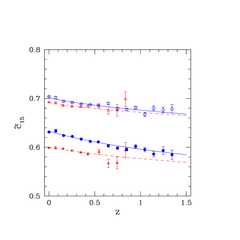
Figure 6.— The redshift dependence of cluster shapes, expressed in terms of the characteristic shape at $10^{15}\hbox{$\,h^{-1}$}{\rm M}_{\odot}$, derived from the combined HV sky survey outputs of the $\Lambda$CDM  (circles) and $\tau$CDM (triangles) models. Filled and open symbols are velocity and position values, respectively. Lines are fits to equation (9), with parameters given in Table 7.

The trend in redshift confirms the expectation that high redshift halos are slightly more ellipsoidal than their counterparts today. The redshift dependence is typically weak, $\varepsilon\!\sim\!0.05-0.09$, with the strongest trend exhibited by the position minor axis of the $\Lambda$CDM model.

The present-epoch mean shapes at $10^{15}\hbox{$\,h^{-1}$}{\rm M}_{\odot}$ are measured independently from the $z\!=\!0$ and sky survey datasets. The correspondence between $\tilde{c}_{15}(0)$ and $\tilde{c}_{15,0}$ to nearly three significant digits implies that our statistical uncertainties are well understood and that there are no systematic differences at this level between the light-cone output used to generate the sky surveys and the more common output produced at fixed proper time.

3.5. Comparisons to Previous Work

Our shape results are generally consistent with previous work, but different techniques for identifying halos, different shape measurement conventions, and variations in assumed cosmology complicate attempts at detailed comparison.

The most recent work that is well aligned with our study is the N-body and particle hydrodynamics simulations of $\Lambda$CDM structure by Suwa et al. (2003). Their cosmological model has slightly higher normalization, $\sigma_{8}\!=\!1$, but is otherwise identical to that assumed in the HV and Virgo $\Lambda$CDM runs. They use a spherical halo definition of somewhat larger radius (defined by an interior density contrast of 200 with respect to the mean, not critical, mass density) and find an average minor axis ratio $\langle\tilde{c}\rangle\!=\!0.62$ for clusters more massive than $2\times 10^{14}\hbox{$\,h^{-1}$}{\rm M}_{\odot}$. Their mass resolution is an order of magnitude improvement over the HV simulations, but their sample contains only 66 objects. Floor et al. (2003) use an annulus method to define projected shapes of halo from several hydrodynamical and N-body simulations. They find an average projected axis ratio of 0.77 at $z\!=\!0$, a value consistent with the mean intermediate axis ratio we find in three dimensions.

Table 7Redshift Dependence of Halo Minor Axis Ratio

Model	Component	$N_{cl}$	$\tilde{c}_{15,0}$	$\varepsilon$
$\Lambda$CDM	Position	44122	$0.633\pm 0.001$	$0.086\pm 0.004$
	Velocity		$0.701\pm 0.001$	$0.053\pm 0.003$
$\tau$CDM	Position	19813	$0.600\pm 0.001$	$0.058\pm 0.007$
	Velocity		$0.691\pm 0.001$	$0.042\pm 0.006$

Other published works employ an ellipsoidal region when defining halo shapes. Warren et al. (1992) applied this technique to ground-breaking, massively parallel simulations and found a distribution of minor axis ratios for galactic-scale halos that peaked at $\tilde{c}\!\simeq\!0.6$, with dispersion $\sim\!0.1$. Thomas et al. (1998) analyze four Virgo simulations, including the two used here, and find mean minor axis ratio $0.50$ with dispersion $\sim\!0.15$ for a sample of 300 halos with mass limit $2\times 10^{14}\hbox{$\,h^{-1}$}{\rm M}_{\odot}$ in low-$\Omega_{m}$ cosmologies. This shape result is significantly more ellipsoidal than our mean value of $0.64$. The difference lies in the shape definition; we use moments of material within a sphere while they use moments of material defined using a percolation algorithm on a set of particles whose local densities lie above a critical threshold. The boundary constraint of our method will tend toward rounder measures while the latter method, because of the directional nature of the percolation process and the pruning in local density, will allow more strongly ellipsoidal values. The degree of difference between the two methods can be large in extreme cases. For the same $\Lambda$CDM Virgo simulations, the most extreme position axis ratio measured by Thomas et al. (1998) is $<0.2$, while the minimum value we derive is a factor two larger $0.4$. Note that the effect in the mean is much smaller, $\sim\!20\%$.

A more complete analysis involves measuring differential shapes as a function of some scale parameter. Warren et al. (1992) used an iterative scheme that began within spheres of fixed physical radius and found a high degree of correlation in direction and shape between $10$ and $40\hbox{$\,h^{-1}$}{\rm\ Mpc}$ in a sample of galactic halos. With much higher resolution simulations, Jing & Suto (2002) employ a sophisticated approach that first measures a local density using a spherical kernel (as in SPH methods, Evrard 1988; Hernquist & Katz 1989), then fits ellipsoids to particles within some narrow range of local density.

From $512^{3}$–particle simulations of a $\Lambda$CDM cosmology, Jing & Suto (2002) measure the distribution of minor axis shapes at a density $2500\rho_{c}$ (corresponding to a radial scale of roughly $\hbox{$r_{200}$}/3$) in a sample of 2494 halos more massive than $6\times 10^{12}\hbox{$\,h^{-1}$}{\rm M}_{\odot}$. They find mean $\langle\tilde{c}\rangle=0.54$ and dispersion $0.11$ at $z\!=\!0$. From analysis of twelve, high-resolution individual halo simulations, they find axial ratios that are rounder at lower densities, with $\tilde{c}\!\sim\!(\rho/\rho_{c})^{-0.052}$. Using this relation to roughly scale to the radius used in this work, $\rho/\rho_{c}\!=\!80$ (equivalent to a mean interior density contrast of 200 for a $\rho\!\propto\!r^{-2.5}$ profile), results in $\langle\tilde{c}\rangle=0.65$ for their mass-limited sample. However, our measurement of the mass dependence of shape implies that a second correction be made in order to infer their expectations at our mass limit of $3\times 10^{14}\hbox{$\,h^{-1}$}{\rm M}_{\odot}$. Using equation (8), the result is an expected mean $\langle\tilde{c}\rangle=0.56$. That the HV sample mean of $0.64$ is significantly larger may again simply reflect the different geometries being used in the two approaches, but this hypothesis remains to tested. Note that the scaled Jing & Suto (2002) result is $0.05$ larger than the mean derived by Thomas et al. (1998) for halos more massive than $2\times 10^{14}\hbox{$\,h^{-1}$}{\rm M}_{\odot}$.

Clearly, there is not a unique measure of absolute halo shape, and future work is needed to more firmly establish the connections between different approaches to shape measurement.

The trends with mass and redshift of the mean minor axis ratio presented in Figures 5 and 6 are in qualitative agreement with Jing & Suto (2002). They find that halos of higher mass (at fixed epoch) and higher redshift (at fixed mass) tend to be more elongated. Their fit to the mass dependence is equivalent to a value $\alpha\!=\!0.02$, in good agreement with our finding of $0.023\pm 0.002$.

Regarding observed trends of cluster shape with redshift, both Plionis (2002) using 903 APM clusters and Melott et al. (2001) using several optical and X-ray cluster samples find trends toward higher ellipticity at increasing redshift. However, Plionis et al. (2004) find a trend of shape with cluster size that is opposite that seen in simulations. From 1168 groups in the UZC-SSRS2 galaxy group catalog, Plionis et al. find that poorer groups are more elongated than richer groups, with $85\%$ of poor groups having $\tilde{b}\lesssim 0.4$. The discrepancy with the models may be due to biases in the optical group catalogs or it may have a physical origin, such as galaxies not fairly sampling the dark matter in low mass systems.

4. SHAPE AND LARGE-SCALE STRUCTURE

For the linear initial density field, a connection between cluster shapes and large-scale structure was established by Bond, Kofman, & Pogosyan (1996), who showed that peaks separated by distances of order the mean inter-peak separation or smaller are likely to have strong connecting filaments. By directing mergers occurring on opposing ends, filaments serve as a source of alignment for halo shapes. Simulations show that this alignment persists into the non-linear regime (van Haarlem & van de Weygaert 1993).

In this section, we present mark correlations of shape, using two measures employed previously by Faltenbacher et al. (2003). We also examine whether clusters that are members of superclusters have shapes that differ from the general population. For the sake of brevity, we present results for the $\Lambda$CDM case only.

4.1. Spatial Correlations of Shapes

Several observational studies have probed the significance and length scale of spatial shape correlations of galaxy clusters. Plionis (1994), using galaxy positions in 637 Abell clusters, presents evidence for nearest neighbor alignment extending to separations $15\hbox{$\,h^{-1}$}{\rm\ Mpc}$ at $\sim\!2.5\sigma$ significance, with weaker alignment to $60\hbox{$\,h^{-1}$}{\rm\ Mpc}$. Fuller, West, & Bridges (1999) used the brightest cluster galaxies (BCG) in poor MKW and AWM clusters and found significant alignments for BCG-cluster pairs and BCG-nearest cluster pairs.

Simulations demonstrate that alignments are to be expected. Using a sample of several hundred clusters more massive than $1.8\times 10^{14}\hbox{$\,h^{-1}$}{\rm M}_{\odot}$ derived from a $512^{3}$–particle $\Lambda$CDM simulation, Onuora & Thomas (2000) detect an alignment signal for pairs extending to $30\hbox{$\,h^{-1}$}{\rm\ Mpc}$, with the strongest signal for nearest neighbors. Like the position–velocity alignments of Figure 3, they note that the signal is persistent and changes little when only strongly elongated halos are used.

Faltenbacher et al. (2003; hereafter F03) examine 3000 clusters more massive than $1.4\times 10^{14}\hbox{$\,h^{-1}$}{\rm M}_{\odot}$ from a $\Lambda$CDM simulation of a $500\hbox{$\,h^{-1}$}{\rm\ Mpc}$ region. They introduce the use of mark correlations to measure the behavior of alignment as a function of radial scale, and find positive signal extending to $15\hbox{$\,h^{-1}$}{\rm\ Mpc}$ and $100\hbox{$\,h^{-1}$}{\rm\ Mpc}$ for two different alignment measures. Hatton and Ninin (2001) measure spatial alignments of halo pair angular momentums that extend to similar scales.

Following F03, we quantify orientation alignment with two different measures. Consider an ensemble of clusters pairs, each with members $i$ and $j$ that have comoving spatial separation $r_{ij}$ between $r$ and $r+dr$. A basic alignment measure (termed ${\cal A}(r)$ by F03) uses the scalar product of major-axis directions $\hat{a}$

$$u(r)\ =\ \bigl{\langle}|\hat{a}_{i}\cdot\hat{a}_{j}|\bigr{\rangle}$$ (10)

where $\langle\ \rangle$ denotes an ensemble average over pairs of separation $r$.

A second, “filamentary” measure (${\cal F}(r)$ of F03) compares halo major-axis orientation to pair separation direction

$$w(r)\ =\ \bigl{\langle}\frac{1}{2}\bigl{(}|\hat{a}_{i}\cdot\hat{r}_{ij}|+|\hat{a}_{j}\cdot\hat{r}_{ij}|\bigr{)}\bigr{\rangle}.$$ (11)

For random halo orientations, both measures have expectation value $u(r)\!=\!w(r)\!=\!0.5$. We therefore use the deviations from this expectation $\delta u(r)\!=\!u(r)-0.5$ and $\delta w(r)\!=\!w(r)-0.5$ as a measure of pairwise alignment.

Figure 7 shows the $\Lambda$CDM position-space alignment signals at $z\!=\!0$ for the sample of 83,000 halos with masses $\hbox{$M_{200}$}\geq 3\times 10^{14}\hbox{$\,h^{-1}$}{\rm M}_{\odot}$. Open circles show $\delta u(r)$ and filled circles give $\delta w(r)$. Error bars are the uncertainty in the binned mean values. For comparison, squares show the two-point spatial correlation function $\xi(r)$ of the mass-limited sample with correlation length $22\hbox{$\,h^{-1}$}{\rm\ Mpc}$ (Colberg et al. 2000). Filled squares show positive spatial correlations while open squares show $|\xi(r)|$ in the region of negative correlations $(\xi(r)<0)$. The inset shows $u(r)$ and $w(r)$ on a linear scale.

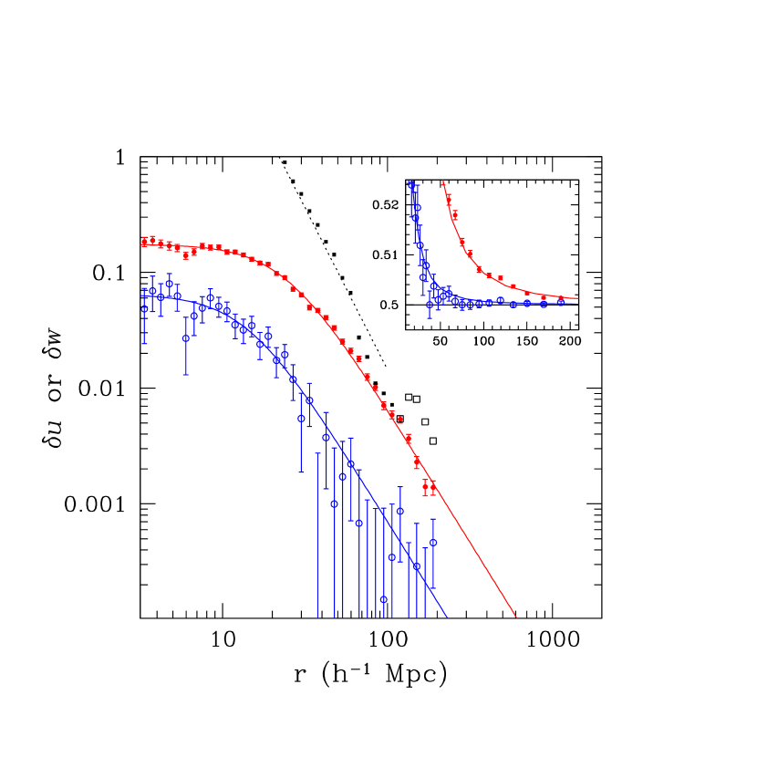
Figure 7.— Mark correlation of cluster orientations as measured by the mean excess basic alignment $\delta u$ (open circles) and the mean excess filamentary alignment $\delta w$ (filled circles) for the HV $\Lambda$CDM sample with $\hbox{$M_{200}$}\geq 3\times 10^{14}\hbox{$\,h^{-1}$}{\rm M}_{\odot}$ at $z\!=\!0$. Solid lines show the fits to equations (12) and (13). Filled squares show the sample’s spatial correlation function in the regime where $\xi(r)>0$ while open squares show $|\xi(r)|$ in the anti-correlated regime. The dotted line is a rough fit of $\xi(r)=(r/22\hbox{$\,h^{-1}$}{\rm\ Mpc})^{-2.8}$ within the range $r\sim 20-60\hbox{$\,h^{-1}$}{\rm\ Mpc}$.

The basic measure shows excess alignment out to scales $\sim\!30\hbox{$\,h^{-1}$}{\rm\ Mpc}$. The filamentary statistic shows non-random halo orientations extending to scales $200\hbox{$\,h^{-1}$}{\rm\ Mpc}$, nearly ten times the correlation length and well into the anti-correlated regime of the two-point function. In both cases, the excess alignment signal is well fit by a power law at large radii that saturates at small $r$. The basic alignments follow

$$\delta u(r)\ =\ 0.065\left(1+\left(\frac{r}{14\hbox{$\,h^{-1}$}{\rm\ Mpc}}\right)\right)^{-2.3}$$ (12)

while the filamentary alignment is well fit by

$$\delta w(r)=0.175\left(1+\left(\frac{r}{24\hbox{$\,h^{-1}$}{\rm\ Mpc}}\right)\right)^{-2.3}.$$ (13)

Our findings are generally consistent with those of F03, but our improved statistics and larger linear scale allow the first detailed fits to the effect. Although an analytic foundation for the specific form of equations (12) and (13) is not yet in hand, we speculate that a solution may be found by applying the theoretical machinery describing peaks in Gaussian random noise fields (Bardeen et al. 1986; Bond & Myers 1996).

F03 note that the filamentary signal remains strong in projection, but their analysis is optimistic in that it assumes perfect knowledge of three-dimensional halo separations as well as the projected three-dimensional halo shapes. A more appropriate treatment will require analysis of galaxy cluster samples derived from mock catalogs (Kochanek & White 2003; Wechsler et al. 2004).

4.2. Supercluster Members

One might reasonably expect local cluster environment to play a role in determining halo shapes. In particular, since superclusters — groups of cluster-mass halos — tend to have strong filamentary morphology, one might anticipate that the formation dynamics of supercluster members may lead to a distribution of shapes that is biased toward more elongated systems.

To address this question, we identify superclusters in the $z\!=\!0$ HV halo population by applying a percolation algorithm with linking length $23\hbox{$\,h^{-1}$}{\rm\ Mpc}$, one-third the $69\hbox{$\,h^{-1}$}{\rm\ Mpc}$ mean intercluster spacing of the sample mass-limited at $3\times 10^{14}\hbox{$\,h^{-1}$}{\rm M}_{\odot}$. We further require that each supercluster have five or more halo members above the mass cutoff. This selects the $8\%$ most strongly clustered halos.

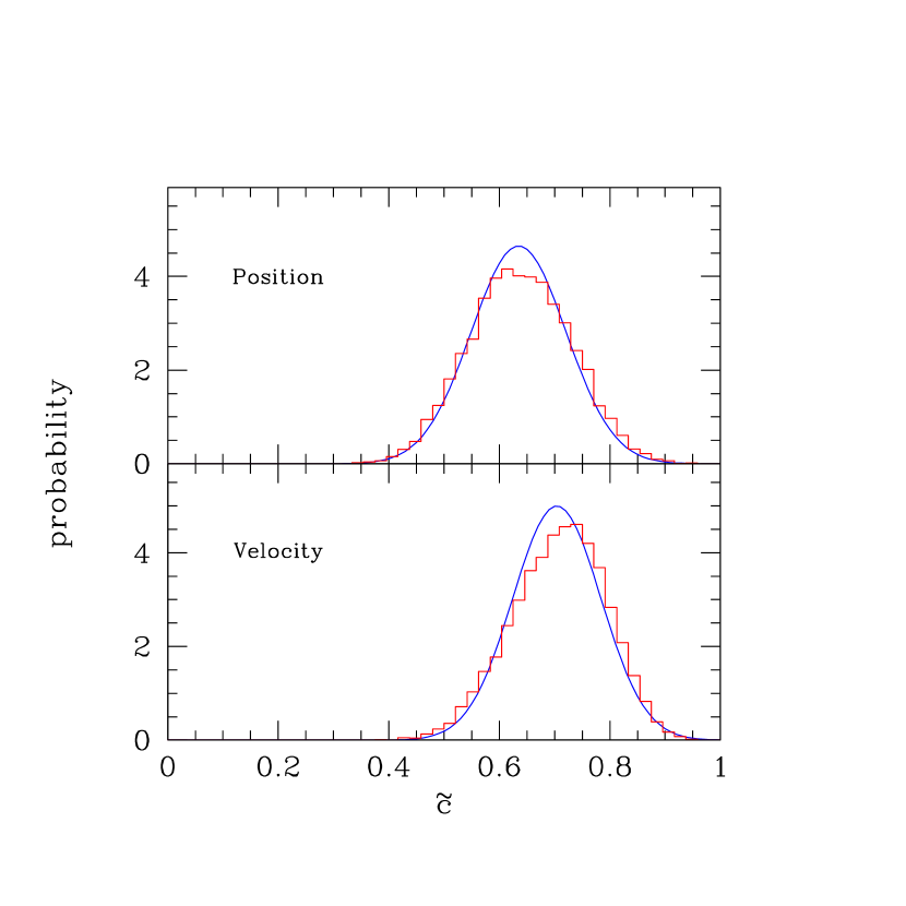
Figure 8.— Distributions of minor axis shapes for the 6683 halos of the $\Lambda$CDM supercluster population (histogram) compared with Gaussian fits to the general population (solid lines) at $z\!=\!0$. A minimum mass of $3\times 10^{14}\hbox{$\,h^{-1}$}{\rm M}_{\odot}$ is employed.

Figure 8 shows the distribution of minor axis ratios in position and velocity for the supercluster members and the general population. The axial ratios of the supercluster population have a nearly Gaussian distribution with means and dispersions presented in Table 8. Comparing supercluster members to the general population (Table 4), we find no difference in mean values at the level of $0.01$ in axial ratio; both have $(\langle\tilde{c}\rangle,\langle\tilde{b}\rangle)=(0.64,0.78)$ in position and $(0.70,0.82)$ in velocity. This finding lends support to the picture in which the halo formation history is largely independent of large-scale environment (Bower 1991; Sheth and Tormen 1999, 2004).

Table 8Supercluster Population Shapes

Model	Ncl	$\tilde{c}$	$\sigma_{\tilde{c}}$	$\tilde{b}$	$\sigma_{\tilde{b}}$
Position	6683	0.638	0.092	0.776	0.096
Velocity		0.704	0.080	0.818	0.088

5. CONCLUSIONS

We use dark matter halos samples from billion–particle N-body simulations to measure statistical properties of halo shapes. The main $\Lambda$CDM samples consist of $83,000$ halos at $z\!=\!0$ and $44,000$ halos from sky survey output with masses $\hbox{$M_{200}$}\geq 3\times 10^{14}\hbox{$\,h^{-1}$}{\rm M}_{\odot}$. For each halo, a moment analysis of density and velocity structure within $r_{200}$ is used to define the principal axes of an equivalent ellipsoid. Higher resolution simulations and random realizations of isothermal spheres demonstrate that systematic errors due to discreteness are less than $0.02$ in mean axial ratio for the main HV samples.

Massive halos have a Gaussian distribution of axis ratios, with intrinsic dispersion $\sim\!0.08$ and a mean minor axis ratio $\langle\tilde{c}\rangle(M,z)\!=\!\tilde{c}_{15,0}\,(1-\alpha\ln M)\,(1+z)^{\varepsilon}$ that tends weakly toward rounder systems at lower mass and redshift ($\alpha\sim\!0.02$ and $\varepsilon\sim\!0.09$ for position, see Tables 6 and 7).

Halos are rounder in velocity than in position space, a finding that likely reflects more efficient scattering in velocity space and the rounder nature of the gravitational potential compared to the density field. The principal axes in position and velocity are strongly correlated; 50% of halos have alignment angles smaller than 22 degrees. We also provide a Gaussian fit to the joint probability density of minor axis ratios in position and velocity.

We investigate mark correlations of cluster shape using two statistics introduced by Faltenbacher et al. (2003). We measure significant excess alignment of halos extending to $30\hbox{$\,h^{-1}$}{\rm\ Mpc}$ for the basic measure and to $200\hbox{$\,h^{-1}$}{\rm\ Mpc}$ for the filamentary statistic. The latter is well fit as a function of scale by $\delta w(r)=0.175[1+(r/24\hbox{$\,h^{-1}$}{\rm\ Mpc})]^{-2.3}$. The filamentary alignment should be detectable in large galaxy cluster surveys such as SDSS, but precise comparison between theory and observation will require a careful study of the connections between clusters observed in redshift/color space and the underlying halo population.

We also find that the distribution of halo shapes in supercluster regions is indistinguishable from that of halos in general, showing that shape is largely independent of large-scale environment.

The statistics presented here can be used to extend approximate methods for creating non-linear representations of the matter distribution based on the halo model description (Scocciamarro and Sheth 2002) by incorporating an ensemble of ellipsoidal halos with correlated orientations and aligned position and velocity ellipsoids.

S.K. acknowledges support from a General Electric Faculty for the Future Fellowship, the Michigan Space Grant Consortium, the Michigan Center for Theoretical Physics, and the Michigan Physics REU Program funded by NSF. A.E. acknowledges support from NASA ATP and NSF ITR grants. We are grateful to Y. Suto, Y. Jing, and M. Plionis for useful comments on an early draft of this paper.

References

- Bardeen et al. (1986) Bardeen, J. M., Bond, J. R., Kaiser, N. & Szalay, A. S. 1986, ApJ, 304, 15
- Binggeli (1982) Binggeli, B. 1982, å, 107, 338
- Binney & Silk (1979) Binney, J. & Silk, J. 1979, MNRAS, 188, 273
- Bond et al. (19966) Bond, J. R., Kofman, L., & Pogosyan, D. 1996, Nature, 380, 603.
- Bond & Myers (1996) Bond, J. R. and Myers, S. 1996, ApJS,103, 1
- Bower (1991) Bower, R. G. 1991, MNRAS, 248, 332
- Carter & Metcalfe (1980) Carter, D. & Metcalfe, N. 1980, MNRAS, 191, 325
- Colberg et al. (2000) Colberg, J. M. et al. 2000, MNRAS, 319, 209
- Cooray & Sheth (2002) Cooray, A. & Sheth, R. 2002, PhR, 372, 1
- de Theije et al. (1995) de Theije, P. A. M., Katgert, P., & van Kampen, E. 1995, MNRAS, 273, 30
- Doroshkevich et al. (1978) Doroshkevich, A. G., Shandarin, S. F., & Saar, E. 1978, MNRAS, 184, 643
- Evrard (1988) Evrard, A. E. 1988, MNRAS, 235, 911
- Evrard et al. (2002) Evrard, A. E. et al. 2002, ApJ, 573, 7