Directional statistics for realistic WIMP direct detection experiments

Abstract

The direction dependence of the event rate in WIMP direct detection experiments provides a powerful tool for distinguishing WIMP events from potential backgrounds. We use a variety of (non-parametric) statistical tests to examine the number of events required to distinguish a WIMP signal from an isotropic background when the uncertainty in the reconstruction of the nuclear recoil direction is included in the calculation of the expected signal. We consider a range of models for the Milky Way halo, and also study rotational symmetry tests aimed at detecting non-sphericity/isotropy of the Milky Way halo. Finally we examine ways of detecting tidal streams of WIMPs. We find that if the senses of the recoils are known then of order ten events will be sufficient to distinguish a WIMP signal from an isotropic background for all of the halo models considered, with the uncertainties in reconstructing the recoil direction only mildly increasing the required number of events. If the senses of the recoils are not known the number of events required is an order of magnitude larger, with a large variation between halo models, and the recoil resolution is now an important factor. The rotational symmetry tests require of order a thousand events to distinguish between spherical and significantly triaxial halos, however a deviation of the peak recoil direction from the direction of the solar motion due to a tidal stream could be detected with of order a hundred events, regardless of whether the sense of the recoils is known.

I Introduction

Weakly Interacting Massive Particle (WIMP) direct detection experiments aim to directly detect non-baryonic dark matter via the elastic scattering of WIMPs on detector nuclei, and are presently reaching the sensitivity required to detect neutralinos (the lightest supersymmetric particle and an excellent WIMP candidate). Since the expected event rates are very small ( ${\cal O}(10^{-5}-1)$ counts ${\rm kg^{-1}day^{-1}}$) distinguishing a putative Weakly Interacting Massive Particle (WIMP) signal from backgrounds due to, for instance, neutrons from cosmic-ray induced muons or natural radioactivity, is crucial. The Earth’s motion about the Sun provides two potential WIMP smoking guns: i) an annual modulation amtheory and ii) a strong direction dependence dirndep of the event rate. In principle the dependence of the differential event rate on the atomic mass of the detector (see e.g. Refs. jkg ; ls ) is a third possibility, however this would require good control of systematics for detectors composed of different materials.

The DAMA (DArk MAtter) collaboration have, using $\sim 100\,{\rm kg}$ of NaI crystals and an exposure of $\sim 1.1\times\,10^{5}\,{\rm kg\,day}$, observed an annual modulation in their event rate dama , which they interpret as a WIMP signal. Taken at face value the allowed region of WIMP mass and cross-section parameter space is incompatible with the exclusion limits from other experiments (such as the Cryogenic Dark Matter Search, Edelweiss and Zeplin I) otherexpt , however the form of the WIMP annual modulation signal, in particular its phase, depends sensitively on the local WIMP velocity distribution amhalo ; amevans ; amhalog1 ; amhalog2  . It is, however, difficult to exclude the possibility that the annual modulation could be due to some previously unidentified background.

The direction dependence of the WIMP scattering rate has several advantages over the annual modulation. Firstly, the amplitude of the annual modulation is typically of order a few per-cent amtheory ; ls while the event rate in the forward direction is roughly an order of magnitude larger than that in the backward direction dirndep ; ls . Secondly it is difficult for the directional signal to be mimicked by backgrounds; in most cases (a point source in the lab is a possible exception) a background which is anisotropic in the laboratory frame will be isotropic in the Galactic rest frame as the, time dependent, conversion between the lab and Galactic co-ordinate frames will wash out any lab specific features. Furthermore the mean direction, in the lab, of WIMP induced recoils will vary over a sidereal day due to the rotation of the Earth dirrot . Designing a detector capable of measuring the directions of sub-100 keV nuclear recoils is however a considerable challenge. Prototype directional detectors based on roton anisotropy in liquid He lhedet , phonon anisotropy in BaF crystals bafdet and the anisotropic scintillation properties of stilbene stildet have been tested, however low pressure gas time projection chambers (TPCs), such as DRIFT (Directional Recoil Identification From Tracks) drift ; sean:drift and NEWAGE newage , seem to offer the best prospects for a workable detector. In discriminating a WIMP signal from isotropic backgrounds it is therefore crucial to take into account the accuracy with which recoil directions can be measured by such a detector. Furthermore, the direction dependence of the recoil rate depends on the local WIMP velocity distribution copi:krauss . Whilst this opens up the exciting possibility of experimentally probing the local dark matter distribution if WIMPs are detected (i.e. doing WIMP astronomy), it is also crucial that uncertainties in this distribution are accounted for when designing tests for discriminating a WIMP signal from isotropic backgrounds.

Earlier studies have found that as few as 30 events would be required to distinguish a WIMP induced signal from isotropic backgrounds copi:krauss ; lehner:dir and that with of order hundreds of events it may be possible to distinguish between different models for the Galactic halo copi:krauss . In this paper we improve on these works by including the uncertainty in the reconstruction of the nuclear recoil direction and applying non-parametric tests to unbinned data. In Sec. II we describe our calculation of the nuclear recoil spectrum, including the modeling of the Milky Way halo (Sec. II.1) and the reconstruction of the recoil direction (Sec. II.2). In Sec. III we then apply an array of statistical tests aimed at probing the isotropy (Sec. III.1), rotational symmetry (Sec. III.2) and mean direction (Sec. III.3) of a putative WIMP directional signal, before concluding with discussion of our results in Sec. IV. In Appendices A, B and C we outline the calculation of the Earth’s orbital velocity, the statistics used and the hypothesis testing formalism respectively.

II Calculating the nuclear recoil spectrum

II.1 Modeling the Milky Way halo

The simplest possible model of the Milky Way (MW) halo is an isotropic sphere with density distribution $\rho\propto r^{-2}$, in which case the velocity distribution at all positions within the halo is maxwellian:

$$f_{0}(\vec{v})=\frac{1}{(2\pi/3)^{3/2}\sigma_{0}^{3}}\exp{\left(\frac{3|\vec{v}|^{2}}{2\sigma_{0}^{2}}\right)}\,,$$ (1)

where $\sigma_{0}$, the velocity dispersion, is related to the asymptotic circular velocity (which we take throughout to be $v_{{\rm c}}=220\,{\rm km\,s}^{-1}$) by $\sigma_{0}=\sqrt{3/2}\,v_{{\rm c}}$.

Observations and numerical simulations indicate that galaxy halos are in fact triaxial and anisotropic and contain substructure. Numerical simulations produce both prolate ($c/b>b/a$) and oblate ($c/b<b/a$) halos (where $(a,b,c)$ are the lengths of the long, intermediate and short principal axes of the density distribution respectively) shape ; js . To date only cluster sized halos have been simulated in large numbers. Ref. js found that the shape parameters of such large halos lie in the ranges $c/a\sim 0.4-0.6$ and $b/a\sim 0.7-0.8$. However the axial ratios vary with radius within a given halo, depending at least partly on the merger history of the halo. Ref. moore:draco studied two high resolution simulations of MW size halos, one halo had $c/a\sim b/a\sim 0.4$, the other $c/a\sim 0.5$ and $b/a\sim 0.8$. These simulations contain only collision-less matter, and the addition of baryons leads to halos that are less triaxial, especially in the central regions sph . These ranges of axial ratios are in rough agreement with observational measurements of the shape of dark matter halos (for reviews see e.g. Ref. shapeobs ).

The two MW-like halos in Ref. moore:draco have velocity anisotropy at the solar radius ($r=R_{0}\approx 8\,{\rm kpc}$) $\beta(R_{0})\sim 0.3\pm 0.1$ where $\beta$ is defined as:

$$\beta(r)=1-\frac{\langle v_{\theta}^{2}\rangle+\langle v_{\phi}^{2}\rangle}{2\langle v_{r}^{2}\rangle}\,,$$ (2)

where $\langle v_{\theta}^{2}\rangle$, $\langle v_{\phi}^{2}\rangle$ and $\langle v_{r}^{2}\rangle$ are the mean square velocity components in Galactic co-ordinates.

II.1.1 Triaxial and anisotropic models

We consider two anisotropic and/or triaxial halo models: the logarithmic ellipsoidal model logellip ; evans and the Osipkov-Merritt model osipkov ; merritt . We summarize these models briefly below. For further details see either the original papers evans ; osipkov ; merritt or Refs. ullio:kamionkowski and  evansomgreen .

The logarithmic ellipsoidal model logellip ; evans is the simplest triaxial, scale free generalization of the isothermal sphere, its shape and velocity anisotropy being independent of radius. This model was studied in detail, in the context of WIMP direct detection, by Evans, Carollo and de Zeeuw evans and has since been used widely in calculations of the expected WIMP signals amevans ; evansomgreen ; amhalog2 . In this model, it is assumed that the principle axes of the velocity distribution are aligned with conical co-ordinates, and in any of the planes of the halo conical co-ordinates coincide with local cylindrical polar co-ordinates and the local WIMP distribution can be approximated by a multi-variate Gaussian:

$$f_{0}(\vec{v})=\frac{1}{(2\pi)^{\frac{3}{2}}\sigma_{R}\sigma_{\phi}\sigma_{z}}\exp\left(-\frac{v_{R}^{2}}{2\sigma_{R}^{2}}-\frac{v_{\phi}^{2}}{2\sigma_{\phi}^{2}}-\frac{v_{z}^{2}}{2\sigma_{z}^{2}}\right)\,,$$ (3)

where $(\sigma_{R},\sigma_{\phi},\sigma_{z})$ are the radial, azimuthal and polar velocity dispersions respectively. These dispersions are given in terms of parameters $p$ and $q$ that are related to the halo axis ratios and $\gamma$ which is related to the isotropy parameter $\beta$ evans ; evansomgreen .

Osipkov-Merritt models osipkov ; merritt provide self-consistent radially anisotropic velocity distribution functions for halos with spherically symmetric density profiles, with velocity anisotropy $\beta(r)=r^{2}/(r^{2}+r_{\rm a}^{2})$ where $r_{\rm a}$ is the anisotropy radius. We follow Ref. ullio:kamionkowski and assume that the MW has an NFW profile NFW with scale radius $20\,$kpc  and fix $r_{\rm a}=20$ and $12\,{\rm kpc}$ as in Ref. evansomgreen , corresponding to $\beta(R_{0})=0.14$ and $0.31$, and calculate the local velocity distribution using the fitting functions in Ref. widrow:fitting .

The parameters of the fiducial halo models which we consider are chosen to span the range of halo properties discussed above and are summarized in Table 1. Some of the triaxial models (numbers 6-9) are rather extreme (with $\sigma_{z}<<\sigma_{r},\sigma_{\phi}$), however they serve as a best/worse case scenario allow us to assess whether the deviation of the recoil spectrum from that produced by the standard halo is detectable/problematic.

II.1.2 Tidal streams

The extent to which the local WIMP distribution is smooth is an open question stiff:widrow:frieman ; moore:draco ; helmi:white:springel ; stiff:widrow2 , however it is certainly possible that a stream of high velocity particles from a late accreted sub-halo could be passing through the solar neighborhood stiff:widrow:frieman ; helmi:white:springel and would produce a potentially distinctive signal in direct detection experiments gondolo:sgr1 . Indeed one of the tidal tails of the Sagittarius dwarf galaxy (Sgr) passes close to the solar neighborhood mass:sgr ; sdss:sgr . Helmi et al. helmi previously discovered a group of halo stars in the solar neighborhood moving coherently with mean velocity in Galactic coordinates $\vec{v}_{\rm str}\approx(-65.0,\,135.0,\,-250.0)\,{\rm km\,s}^{-1}$ and Freese et al. gondolo:sgr2 have argued that these stars are in fact part of the Sgr tidal stream. This interpretation is somewhat controversial. Firstly (as noted by Freese et al.) there is a discrepancy between the measured velocity of these stars and that expected for the Sgr stream. Secondly, there is a second lower density stellar stream in the solar neighborhood moving in the opposite direction helmi which is not expected for debris associated with Sgr. Finally the comparison of detailed simulations of the kinematics of the Sgr stream with measured radial velocities of Sgr stream stars appears to indicate that the stream does not pass through the solar neighborhood helmi2 .

None the less there is a debris stream passing through the solar neighborhood regardless of whether or not it originated from the Sgr dwarf galaxy. We therefore follow Ref. gondolo:sgr1 ; gondolo:sgr2 and assume that there is dark matter associated with the stream and model its velocity distribution of WIMPs as a maxwellian distribution with bulk velocity $\vec{v}_{\rm str}$, and velocity dispersion $\sigma_{\rm str}$:

$$f_{0}(\vec{v})=\frac{1}{(2\pi/3)^{3/2}\sigma_{\rm str}^{3}}\exp\left(-\frac{3|\vec{v}-\vec{v}_{\rm str}|^{2}}{2\sigma_{\rm str}^{2}}\right)\,.$$ (4)

We take $\sigma_{\rm str}=30\,{\rm km\,s}^{-1}$, and $\rho_{0}=0.07\,{\rm GeV\,cm}^{-3}(\approx 0.25\rho_{0})$, (towards the lower and upper ends of the range of values suggested in Ref.  gondolo:sgr1 ; gondolo:sgr2 respectively and therefore providing a best case scenario for detectability), and for simplicity use the standard maxwellian velocity distribution [eq. (1)] for the smooth background component.

No.	Type	p	q	$\beta$	axis	$\rho_{\rm str}/\rho_{0}$	$\sigma_{\rm str}$ (km   s-1)
1	SHM	-	-	-	-	-	-
2	LGE	0.9	0.8	0.1	I	-	-
3	LGE	0.9	0.8	0.4	I	-	-
4	LGE	0.9	0.8	0.1	L	-	-
5	LGE	0.9	0.8	0.4	L	-	-
6	LGE	0.72	0.7	0.1	I	-	-
7	LGE	0.72	0.7	0.4	I	-	-
8	LGE	0.72	0.7	0.1	L	-	-
9	LGE	0.72	0.7	0.4	L	-	-
10	OM	-	-	0.31	-	-	-
11	OM	-	-	0.14	-	-	-
12	SHM.+Str	-	-	-	-	0.25	30

Table 1: Summary of the parameters of the fiducial halo models. ‘SHM’ denotes the standard halo model, ‘LGE’ the logarithmic ellipsoidal model with the Sun located on either the long (L) or intermediate (I) axis, ‘OM’ the Osipkov-Merritt model and ‘SHM+ Str’ the standard halo model plus tidal stream contributing $\rho_{\rm str}/\rho_{0}$ of the local WIMP density, with bulk velocity and velocity dispersion as described in the text. In each case we take $v_{{\rm c}}=220\,{\rm km\,s}^{-1}$ and $\beta$ is the anisotropy parameter, defined as in eq. (2).

II.2 Modeling the detector response

TPC based detectors are designed to measure the directions of nuclear recoils by drifting the ionisation produced by recoils in the gas volume to a suitable charge readout plane. The difference in ionisation track lengths between electrons, alpha particles and nuclear recoils at low gas pressure allows efficient rejection of these backgrounds drift . To reduce charge diffusion along the track (which would restrict the spatial resolution and hence direction measurement and background discrimination) to thermal levels the detector can be filled with an electronegative gas to give negative ion drift. The DRIFT collaboration have adopted CS₂ as a suitable electronegative gas; for further details see Ref. drift ; sean:drift .

The recoiling nucleus undergoes a large number of scatterings (on average 30 (70) for a primary recoil energy of 20 (100) keV, with a gaussian distribution). These multiple scatterings together with the small, but finite, diffusion of drifted ionisation limits the accuracy with which the direction of the primary recoil can be reconstructed. In order to assess the likely accuracy of the track reconstruction we consider a TPC detector filled with 0.05 bar CS₂ with a 200$\,\mu$m pitch micropixel readout plane, a 10cm drift length over which a uniform electric field of $1\,{\rm kV\,cm}^{-1}$ is applied. This gas pressure, mixture and electric field are chosen to match the design of the DRIFT-I detector sean:drift . The micropixel readout is based on those described in Ref. bellazini , and the drift length is such that the rms diffusion over the full drift length is approximately equal to the pixel pitch ohnuki . We use the SRIM2003 package srim   to generate sulfur ionisation recoil tracks  We simulate the drift and diffusion of the ionisation to the readout plane under the electric field and the subsequent generation of charge avalanches. The quenching factor (fraction of recoil energy going into ionization) is roughly 0.4 for a primary recoil energy of 20 keV, in agreement with experimental data quench , however the direction reconstruction depends on the electron distribution and not their number.

The charge distributions are then projected into the xy, yz and xz planes (as illustrated in Fig. 1). The resulting pixel hit pattern is approximately elliptical with long axis close to the primary recoil direction, which allows us to reconstruct the nuclear recoil directions via a moment analysis. The distribution of the difference between the primary recoil direction and the reconstructed track direction peaks at $\sim 15^{\circ}$, decreasing weakly with increasing energy, and has a long large angle tail (the mean and root mean square deviation are $\sim 25^{\circ}$ and $\sim 15^{\circ}$, again weakly decreasing with increasing energy). We include this stochastic uncertainty in our Monte Carlo simulations.

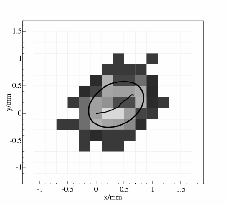
Figure 1: Simulated pixel read-out in the xy plane from a 40keV recoil. The strength of the signal in each pixel is obtained by integrating the voltage pulse for that pixel. The actual recoil track is shown by the solid line. The ellipse results from the moment analysis and its long axis gives the reconstructed direction.

The primary recoil energy threshold is 20 keV as below this energy the short track length ( 3-4 pixels) and multiple scatterings make it impossible to reconstruct the track direction. With SRIM2003 generated recoils, we find near uniform distributions of ionisation along the tracks and therefore cannot determine the absolute signs of the reconstructed recoil vectors (i.e $+\vec{x}$ or $-\vec{x}$). However, we note that experimental measurements are really required to determine whether this absolute sign can be measured or not. We consider both possibilities below.

We assume that the time-dependent conversion of recoil directions measured in the laboratory frame to the galactic frame introduces no further errors in the measured recoil directions due to, for instance, inaccuracy in the measured time of the event.

We calculate the directional recoil rate above the $20\,{\rm keV}$ detector energy threshold via Monte Carlo simulation so as to allow the inclusion of the detector resolution effects discussed above. We work in Galactic $(R,\phi,z)$ co-ordinates, where $R$ is directed towards the Galactic center, $\phi$ is in the direction of motion of the Local Standard of Rest (LSR) and $z$ points towards the north Galactic pole. These co-ordinates are related to Galactic longitude $l$ and latitude $b$ by $(R,\,\phi,\,z)=(\cos{l}\cos{b},\sin{l}\cos{b},\sin{b})$.

Firstly the WIMP velocity distribution has to be transformed to the rest frame of the detector $[f_{0}(\vec{v}_{\chi})\rightarrow f_{\oplus}(\vec{u}_{\chi})]$ via the Galilean transformation: $\vec{v}_{\chi}=\vec{u}_{\chi}+\vec{v}_{\oplus}(t)$. The velocity of the Earth, $\vec{v}_{\oplus}(t)$, is the sum of the velocity of the LSR, $\vec{\Theta}_{LSR}$, the peculiar velocity of the Sun, $\vec{v}_{\odot p}$, and the Earth’s orbital velocity about the Sun, $\vec{v}_{orb}(t)$. We take $\vec{\Theta}_{LSR}=220\,{\rm km\,s}^{-1}$ (see e.g. binney:tremaine ), $\vec{v}_{\odot p}=(10.0,7.3,5.2)\,{\rm km\,s}^{-1}$ dehnen:binney:hipparcos , and use the results of the calculation of the Earth’s orbital velocity detailed in Appendix A. The resulting WIMP velocity distribution in the detector rest frame is used to generate random incident WIMP velocities from the WIMP flux $u_{\chi}f_{\oplus}(\vec{u}_{\chi})$, which then undergo isotropic scattering in the center of mass frame. We weight each recoil by a factor equal to the detector form factor (which is taken to have the Helm form appropriate for spin independent WIMP-sulfur scattering ls ) in order to take into account the variation of the scattering cross section with the momentum transfer to the nucleus. Finally we include the effects of multiple scattering on the reconstructed recoil direction.

The resultant, time averaged, WIMP and recoil distributions are shown as Hammer-Aitoff projections of the flux/rate in Galactic coordinates in Figs. 2-4 for models 1 (standard halo model), 3 (logarithmic ellipsoidal model with $p=0.9,q=0.8$ and $\beta=0.4$ ) and 12 (standard halo model with a 25$\%$ contribution to the local WIMP density from a tidal stream with properties as described in Sec. II.1.2). For illustrative purposes we take $\rho_{0}=0.3\,{\rm GeV\,cm}^{-3}$, $m_{\chi}=100\,{\rm GeV}$ and for the recoil flux take the WIMP-proton elastic scattering cross-section to be $\sigma_{\chi p}=10^{-6}\,$pb. Note the different scale for model 12. We see that the WIMP flux produced by the triaxial halo model is significantly flattened with respect to the Galactic plane, however due to the finite detector resolution the difference between the recoil rates predicted by models 1 and 3 is far smaller than the difference in the WIMP fluxes. For model 12, with the tidal stream, the peak direction of the WIMP flux and recoil rate both differ significantly from the direction of motion of the Sun, suggesting that WIMPs associated with the stream of halo stars in the solar neighborhood could be detectable in a directional detector if the WIMP density is sufficiently large.

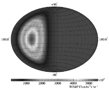
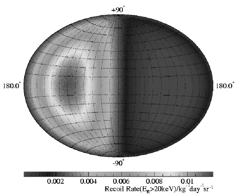
Figure 2: Time averaged WIMP flux (top) and S Recoil rate above $20\,{\rm keV}$ (bottom) in Galactic $(l,b)$ co-ordinates for halo model 1 and $\rho_{0}=0.3\,{\rm GeV\,cm}^{-3}$, $m_{\chi}=100$ GeV and $\sigma_{\chi p}=10^{-6}$ pb.

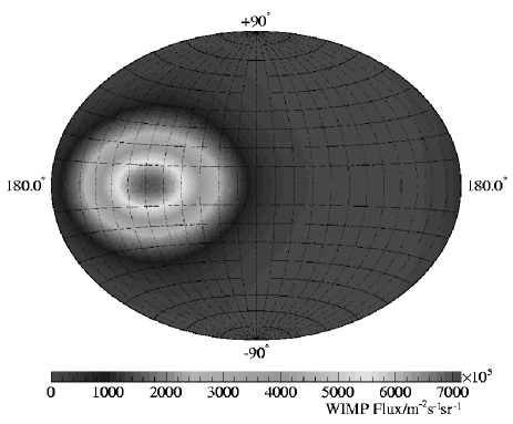
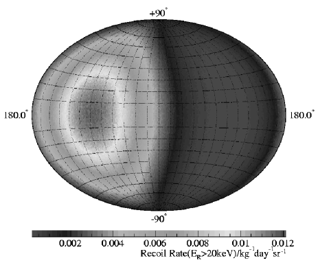
Figure 3: As Fig. 2 for model 3 (logarithmic ellipsoidal model with $p=0.9,q=0.8$ and $\beta=0.4$ ).

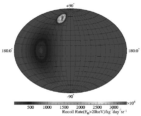
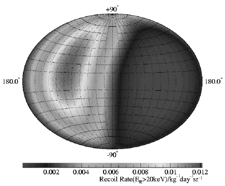
Figure 4: As Fig. 2 for model 12 (standard halo model with a 25$\%$ contribution to the local WIMP density from a tidal stream with properties given in Sec. II.1.2).

III Applying Statistical tests

A WIMP search strategy with a directional detector can essentially be divided into three regimes. Firstly, there is the simple search phase which aims to detect an anomalous recoil signal above that expected from backgrounds. Secondly, following the discovery of an anomalous recoil signal, there would be the confirmation stage. At this point the experiment would collect more data and aim to confirm the recoil signal as Galactic in origin by searching for the expected anisotropy in the recoil directions. In statistical terms the question posed at this point is ‘Is the distribution of observed recoil directions isotropic?’, more specifically ‘How many events are required to reject the hypothesis of isotropy (at a given confidence level)?’. Thirdly, assuming anisotropy is detected, the experiment would then collect more data and try and determine the form of the recoil anisotropy and hence the local WIMP velocity distribution. The halo models considered in Sec. II.1 lead us to consider two simple hypotheses to test: 1) Does the distribution of recoil directions show evidence of flattening (i.e. a non-spherical halo)? and 2) Does the distribution of recoil directions show evidence for a signal from a tidal stream?

As discussed in Sec. I, previous work aimed at determining the number of events required to detect the anisotropy in the recoil directions has indicated that $5-30$ events are required to give a 90-95% rejection of isotropy copi:krauss ; lehner:dir . However, these analyses suffer from several non-optimal features. Neither analysis took into account the angular resolution of the recoil reconstruction or the possibility that the absolute signs of the recoil vectors (i.e. their ‘sense’ $+\vec{x}$ or $-\vec{x}$) may not be measurable. In Ref. lehner:dir , a Kolmogorov-Smirnov goodness of fit test was applied to the binned distribution of recoil $\cos\gamma$ values, where $\gamma$ is the angle between the recoil direction and the direction of motion of the Sun. Given the small number of events expected at the confirmation stage of an experiment, binning data can lead to a significant loss of information and should therefore be avoided. Ref. copi:krauss used an unbinned likelihood analysis to determine the number of events required for a 95% confidence detection of isotropy in 95% of experiments, for a range of halo models, and also the number of events required to distinguish a triaxial halo from the standard maxwellian halo model. The draw-back of likelihood analysis is that it requires the likelihood function for the recoil distribution generated by a given halo model. It can therefore only give the relative likelihood of specific models (and parameter values), and there is no guarantee that any of the halo models considered is a good approximation to the local WIMP velocity distribution (especially since non-spherical and/or anisotropic halo models involve assumptions, which may or not be valid). As such this analysis could not be applied to real data.

Recoil directions constitute vectors, or, if the senses are unknown, undirected lines or axes, and so can equivalently be represented as points on a sphere. This allows us to use statistical inference methods developed for the analysis of spherically distributed data (for a review of this extensive field see the standard texts such as mardia:jupp ; fisher:lewis:embleton ). We investigate a variety of non-parametric statistics designed to test the isotropy (Secs. III.1), rotational symmetry (Sec. III.2) and median direction (Sec. III.3). When quoting results for the numbers of events required for detection, we focus on the benchmark halo models discussed in Sec. II.1, however these tests do not make any assumptions about the form of the recoil spectrum and are hence equally applicable to any local WIMP velocity distribution. Recoil energies are not incorporated in these statistics, but the energy provides no extra information about the degree of anisotropy and/or rotational symmetry in the data. In addition, any analysis including the recoil energy would require (halo model dependent) assumptions about the form of the recoil energy spectrum as a function of direction.

Throughout we assume zero background. This is a reasonable expectation for experiments such as DRIFT-II made from low activity materials with efficient gamma rejection and shielding drift2:design . However, non-zero backgrounds can be incorporated into the statistical tests. For real data, one would simply calculate the value of the appropriate test statistic using the observed sample of recoil vectors/axes and use its null distribution (Appendix B1) to determine the probability of the sample being isotropic. No assumption about the level of background contribution to the sample is neccessary, but there is an implicit assumption that background event directions are isotropically distributed.

In the case of our simulations, it would be neccesary to fix the background rate and exposure so that the expected number of background events $N_{b}$ is known. A variable number of WIMP events $N_{\rm w}$ can then be added to the $N_{\rm b}$ background events, and the formalism of Appendix C used to determine the value of $N_{\rm w}$ required to reject isotropy of the $N_{\rm w}+N_{\rm b}$ recoil sample at a given confidence level. Since the background rate and exposure are dependent on the experiment, investigating the effect of varying background rates is beyond the scope of this paper. Therefore, and given that the next generation of directional detectors are expected to have essentially zero background drift2:design , we assume zero background to provide benchmark figures. Nevertheless, the formalism presented in this paper could be used to predict the directional sensitivity of a detector with non-zero background once the background rate and exposure have been estimated.

III.1 Tests of isotropy

The first fundamental question posed by a directional detector observing an anomalous recoil signal is ‘Are the observed recoil directions consistent with an isotropic distribution?’. The most general tests of isotropy are those which do not depend on the coordinate system in which the sample vectors/axes are measured. This independence from the coordinate system means no assumption about the form of the anisotropy in the signal is required. While this is usually an advantage, coordinate independent tests cannot make use of any information that is available about the expected form of the anisotropy. If the local WIMP distribution is smooth then the year averaged recoil flux will be peaked in the direction of the Sun’s motion at $(l_{\odot},b_{\odot})=(87.5^{\circ},1.3^{\circ})$.

For each of the statistics discussed in Appendix B.1 we determine the minimum number of events required to reject isotropy of recoil directions at $90\,(95)\%$ confidence in $90\,(95)\%$ of experiments (i.e. for rejection and acceptance probabilities of $R_{\rm c}=A_{\rm c}=0.9$ and $0.95$), $N_{\rm iso}$, as described in Appendix C, for each statistic and halo model considered, including the detector response in the calculation of the recoil distributions. For the standard maxwellian halo model we also carry out the calculation neglecting the reconstruction uncertainty and for a hypothetic perfect detail which also has zero energy threshold , in order to assess the effect of the reconstruction uncertainties and the finite energy threshold on the number of events required. The results are tabulated in Table 2 for each of the fiducial halo models for each statistic.

Halo	$N_{\rm iso}$ for $(R_{\rm c},A_{\rm c})=(0.90,0.90)$
Model	Vectorial Statistics				Axial Statistics
	${\cal W}^{\star}$	${\cal A}$	${\cal F}$	$\langle\cos\theta\rangle$	${\cal B}^{\star}$	${\cal G}$	$\langle|\cos\theta|\rangle$
1	12	12	13	7	165	167	81
1 (no)	10	10	10	5	83	84	40
1 (per)	18	18	18	10	531	538	258
2	12	12	12	7	114	114	57
3	14	14	15	8	157	159	93
4	12	12	13	7	149	151	74
5	14	14	15	8	157	159	93
6	11	11	11	6	67	67	36
7	14	14	14	8	88	90	57
8	13	13	14	7	175	178	86
9	15	15	16	9	264	267	146
10	15	15	16	8	280	284	149
11	12	12	12	7	125	126	62
12	14	14	14	8	221	222	159
	$N_{\rm iso}$ for $(R_{\rm c},A_{\rm c})=(0.95,0.95)$
1	18	18	19	11	235	235	131
1 (no)	13	13	14	9	120	120	65
1 (per)	25	25	26	15	767	769	426
2	17	17	18	10	161	163	93
3	20	20	21	12	225	224	152
4	18	18	19	11	215	214	120
5	20	20	21	12	222	22	153
6	16	16	16	10	96	97	59
7	19	20	20	12	125	125	93
8	18	18	19	11	252	252	142
9	21	21	22	13	378	383	241
10	21	21	21	12	402	405	247
11	17	17	17	10	180	182	102
12	19	19	20	12	316	320	264

Table 2: Number of recoil events required to reject isotropy of recoil directions, $N_{\rm iso}$, at $90\,(95)\%$ confidence in $90\,(95)\%$ of experiments for each test statistic and halo model considered, including the uncertainty in the nuclear recoil reconstruction and for the standard halo model ignoring the uncertainty in the nuclear recoil reconstruction (denoted by ‘no’ in the table) and for a hypothetical perfect detector with zero threshold and no reconstruction uncertainities (denoted by ‘per’). The test statistics have been divided into those suitable for vectorial data and those applicable to axial data (i.e. when the senses of the recoil directions are not known).

Overall, the two coordinate dependent tests of isotropy, $\langle\cos\theta\rangle$ and $\langle|\cos\theta|\rangle$, have the lowest $N_{{\rm iso}}$ values and are thus the most powerful tests for rejecting isotropy. All the coordinate independent tests typically require 1.5-2 times more events to reject isotropy for a given halo model (for both vectorial and axial data). This is perhaps not surprising for the models 1-11 however, the coordinate dependent tests are also the most powerful for rejecting isotropy in model 12 which includes a $25\%$ contribution to the local WIMP density from a tidal stream.

The vectorial coordinate independent tests (${\cal W}^{\star}$, ${\cal A}$ and ${\cal F}$) all have very similar values of $N_{{\rm iso}}$ and are hence equally powerful for rejecting isotropy of recoils. The same is true of the axial coordinate independent tests (${\cal B}^{\star}$ and ${\cal G}$), however $N_{{\rm iso}}$ is of order ten times larger for these tests than for the vectorial tests, and there is much greater variation between the fiducial halo models. Both of these effects are due to the form of the recoil direction distribution and the way in which lack of knowledge of the recoil sense changes this form. While most of the recoil arrival directions lie in the forward hemisphere, $0<l<180^{\circ}$, a non-negligible (halo model dependent) number lie in the backward hemisphere. For the vectorial tests, these backward events are not a problem as the tests can distinguish between the forward and backward hemispheres. When only the recoil axis is known, events in the backward hemisphere are effectively ‘added’ to the forward hemisphere, reducing the degree of anisotropy. Halo model 6 has the smallest rate in the backward hemisphere and thus the lowest $N_{{\rm iso}}$ for both vectorial and axial tests, while model 10 has the largest backward rate and therefore has higher $N_{{\rm iso}}$ values with axial tests. In general the broader the local WIMP velocity distribution, the greater the number of events in the backward hemisphere, and hence a larger number of events are required to reject isotropy if the sense of the recoil directions are not known.

Ignoring the detector response only marginally reduces the number of events required for the vectorial tests, however the number of events required for the axial tests are decreased by a factor of roughly two. For the hypothetical detector with perfect reconstruction and zero energy threshold the number of events required increases, relative to the 20 keV perfect reconstruction case, by a factor of $\sim 2(\sim 6)$ for the vectorial (axial) statistics. The number of events required increases since, as is well known dirndep , the anisotropy of the recoil directions decreases with decreasing recoil energy. The total recoil rate with a 0 keV threshold is roughly twice that with a 20 keV threshold, therefore for the vectorial statistics the exposure required to detect a WIMP signal is essentially unchanged, while for the axial statistics (i.e. if it is not posible to measure the senses of the recoils) the lower threshold would actually increases the exposure required.

We now translate the number of events required to reject isotropy for the realistic detector into the equivalent detector exposure, $E$, required to observe this number of events. If the senses of the recoil directions are observed, isotropy could be rejected at $95\%$ confidence in $95\%$ of experiments for $\sigma_{0}\sim 3\times 10^{-9}\,{\rm pb}$ and $\rho_{0}\sim 0.3\,{\rm GeV\,cm}^{-3}$ with an exposure of $E\sim 10^{5}\,{\rm kg\,day}$ (i.e. a 100 kg detector operating for a period of 2-3 years). For a detector only capable of measuring the recoil axes a $10^{5}\,{\rm kg\,day}$ exposure would be able to reject isotropy at the same confidence level and acceptance down to $\sigma_{0}\sim 3\times 10^{-8}\,{\rm pb}$.

III.2 Tests for rotational symmetry

Once an observed anomalous recoil signal is found to be incompatible (at some confidence level) with isotropy the next question to pose is ‘Is the observed distribution consistent with a spherical halo?’. A generic feature of triaxial halo models is a flattening of the recoil distribution towards the galactic plane, or more generally, flattened along one principal axis of the local velocity distribution. This type of distribution can be probed using tests for rotational symmetry about a specified direction or axis. In the case of smooth halo models this direction/axis is the direction of motion of the Earth through the MW halo, which over the year, averages to the direction of motion of the Sun, $(l_{\odot},b_{{\odot}})$ .

We focus here on the two fiducial halo models for which the recoil distribution deviates most from that produced by the standard halo model: the logarithmic ellipsoidal models 5 ($p=0.9$, $q=0.8$, $\beta=0.4$, long axis) and 7 ($p=0.72$, $q=0.7$, $\beta=0.4$, intermediate axis)   and find the number of events required to reject rotational symmetry, $N_{{\rm rot}}$, using the Kuiper statistic ${\cal V}^{\star}$ as defined in Appendix B.2. We find that halo model 5 has $A<0.4$ over a large range of $N$ values, and of order 5000-8000 events would be required to reject rotational symmetry at $90+\%$ confidence with similar acceptance. In contrast for halo model 7 (which is more extreme) $N_{{\rm rot}}=1170\,(1710)$ for $R_{\rm c}=A_{\rm c}=0.9\,(0.95)$. So while rotational symmetry of the recoil distribution can be rejected at high confidence and acceptance for this, rather extreme, halo model, it requires 10-50 times the number of events required to reject isotropy (depending on whether vectors or axes are measured in the latter case).

Converting these numbers to the equivalent exposures in ${\rm kg\,day}$ gives $E(R_{\rm c}=A_{\rm c}=0.9\,(0.95))=7.8\,(11)\times 10^{-3}\sigma_{0}^{-1}\rho_{0}^{-1}$. Hence for the $10^{5}\,{\rm kg\,day}$ exposure considered in the previous subsection, rotational symmetry could be rejected at $90\%$ confidence down to $\sigma_{0}\sim 3\times 10^{-7}\,{\rm pb}$ for $\rho_{0}\sim 0.3\,{\rm GeV\,cm}^{-3}$, independent of whether the senses of the recoils can be measured. The sensitivity of a TPC-based directional detector for rejecting a spherical halo if the real MW halo is significantly triaxial using this statistic, is therefore several orders of magnitude lower than for rejecting isotropy of recoil directions. Devising other tests that may be a more powerful probe of the flattening of the recoil distribution produced by non-spherical halo models is therefore an important task.

III.3 Tests for mean direction

Tidal streams will typically have a velocity dispersion which is small compared to their velocity relative to the solar system and therefore the recoil distribution due to WIMPs from a stream will be peaked in the hemisphere whose pole points in the direction of the stream velocity. The net (stream plus smooth background WIMP distribution) peak direction depends on the fraction of the local density that the tidal stream contributes. Fig. 5 shows the angle between the direction of the Sun’s motion $(l_{\odot},b_{\odot})=(87.5^{\circ},1.3^{\circ})$ and the direction of the peak in the recoil distribution produced by a maxwellian halo plus a stream with velocity $\vec{v}_{\rm str}=(-65.0,\,135.0,\,-250.0)\,{\rm km\,s}^{-1}$ as a function of the local WIMP density contributed by the stream. For the $\rho_{\rm str}/\rho_{0}\sim 1-30\%$ range of stream densities suggested by gondolo:sgr1 ; gondolo:sgr2 , the angle is in the range $2-15^{\circ}$. This feature suggests that the presence of a WIMP stream in the solar neighborhood could be tested for by comparing the median direction of the observed recoil vectors with the (known) direction of solar motion.

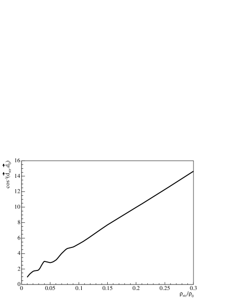
Figure 5: Variation of the angle (in degrees) between the mean recoil directions of the standard halo and the standard halo plus a tidal stream with $\vec{v}_{\rm str}=(-65.0,\,135.0,\,-250.0)\,{\rm km\,s}^{-1}$ function of the fraction of the local WIMP density contributed by the stream, $\rho_{\rm str}/\rho_{0}$.

For $\rho_{\rm str}/\rho_{0}=25\%$ (which is at the upper end of the range of values suggested in gondolo:sgr2 ; gondolo:sgr1 , and therefore provides a lower limit on the number of events required), we find that the minimum number of events required to reject $(l_{\odot},b_{\odot})$ as the median direction, $N_{\rm dir}$, using the ${\cal X}^{2}$ test as defined in Appendix B.3 is $201\,(294)$ for $R_{\rm c}=A_{\rm c}=0.9\,(0.95)$. Comparing these numbers with those required to reject isotropy of recoils for this stream density, it can be seen that $\sim 10-20$ times more events are needed to reject the direction of the solar motion as the median recoil direction. These numbers of events would be achievable with a $10^{5}\,{\rm kg\,day}$ exposure for WIMP-proton cross sections down to $\sigma_{0}\sim 4\times 10^{-8}\,(6\times 10^{-8})\,{\rm pb}$ for $\rho_{0}=0.3\,{\rm GeV\,cm}^{-3}$.

In the case of axial recoil directions, the ${\cal X}^{2}$ test cannot be applied, however, the rotational symmetry test presented in Appendix B.2 can be used since the recoil distribution will not be rotationally symmetric about $(l_{\odot},b_{\odot})$ in the presence of a stream and we find $N_{\rm rot}=390\,(574)$ for $R_{\rm c}=A_{\rm c}=0.9\,(0.95)$. These numbers are roughly twice those for the ${\cal X}^{2}$ test, and also for rejecting isotropy with axial data. Thus with only axial data, a $10^{5}\,{\rm kg\,day}$ exposure would be sufficient to identify the presence of a tidal stream with properties as described in Sec. II.1.2 comprising $25\%$ of the local WIMP density for WIMP-proton cross sections down to $\sigma_{0}\sim 8\times 10^{-8}\,(1\times 10^{-7})\,{\rm pb}$ and $\rho_{0}=0.3\,{\rm GeV\,cm}^{-3}$.

We caution that these numbers have been calculated for parameter values at the optimistic ends of the ranges estimated in Ref. gondolo:sgr1 ; gondolo:sgr2 , i.e. high density and low velocity dispersion. A lower stream density and/or a higher velocity dispersion would give a peak recoil direction closer to the mean direction of motion of the Sun, and make the deviation due to the stream harder to detect. For the most pessimistic case of $\rho_{\rm str}/\rho_{0}=0.003$ and $\sigma_{\rm str}=70\,{\rm kms^{-1}}$, the net WIMP flux and recoil rate are virtually indistinguishable from those for the standard halo model and tens of thousands of events would be needed to detect the stream. In general the directional detectability of cold streams of WIMPs will clearly depend on how much their bulk velocity deviates from the direction of solar motion.

IV Discussion

We have studied the application of non-parametric tests, developed for the analysis of spherical data mardia:jupp ; fisher:lewis:embleton , to the analysis of simulated data as expected from a TPC-based directional WIMP detector drift ; sean:drift , taking into account the uncertainties in the reconstruction of the nuclear recoil directions. These tests, unlike likelihood analysis, do not require any assumptions about the form of the local WIMP velocity distribution. This is advantageous as even if the properties (i.e. shape, velocity anisotropy, and density profile) of the MW halo at the solar radius were accurately determined there would likely be a wide range of local velocity distributions consistent with these properties.

For a range of fiducial anisotropic and/or triaxial halo models, with parameters chosen to reproduce the range of properties found in simulations/observations of dark matter halos, we calculate the number of events required to distinguish the WIMP directional signal from an isotropic background using a variety of tests. The most powerful test is the, co-ordinate system dependent, test of the mean angle between the observed nuclear recoils and the direction of motion of the Sun, which takes advantage of the fact that, for a smooth halo, the recoil rate is peaked in the direction of the Sun’s motion. We find that if the senses of the recoils are known then of order ten events will be sufficient to distinguish a WIMP signal from an isotropic background for all of the halo models considered, with the uncertainties in reconstructing the recoil direction only mildly increasing the required number of events. If the senses of the recoils are not known the number of events required is an order of magnitude larger, with a large variation between halo models and the recoil resolution is now an important factor. The number of events required would be significantly larger if the WIMP velocity distribution in the rest frame of the detector is close to isotropic copi:krauss , which could be the case if the MW halo is co-rotating or if the local dark matter density has a significant contribution from a cold flow with direction so as to cancel out the front-rear asymmetry from the smooth background distribution sikivie , however for halos formed hierarchically (as is the case in Cold Dark Matter cosmologies) neither of these possibilities are expected to occur (see e.g. Ref. moore:draco ; helmi:white:springel ). Our conclusions for the case where the recoil senses are known are in broad agreement with the results of Ref. copi:krauss . It is reassuring that the realistic modeling of detector properties and the use of statistics that can be applied to real data do not significantly degrade the expected detection power of directional experiments.

Halo models which produce significantly different WIMP flux distributions, unfortunately give very similar recoil rates. We find that distinguishing between halo models, in particular determining whether the MW halo is (close to) spherical, using tests of rotational symmetry will require thousands of events.

Gondolo has shown that the recoil momentum spectrum is the Radon transform of the WIMP velocity distribution gondolo . In theory the transform could be inverted to directly measure the WIMP velocity distribution from the measured recoil momentum distribution, however the inversion algorithms available in the literature require large numbers of events gondolo . Furthermore, as we have shown, the uncertainties in the reconstruction of the recoil directions due to multiple scattering and diffusion have a significant effect on the observed recoil distribution and it is not possible to apply this inversion to real data. Developing techniques to distinguish between the recoil distributions expected from different halo models, for finite amounts of data and taking into account the experimental resolution, is therefore of key importance for the full astronomical exploitation of data from directional detectors.

If a significant fraction of the local dark matter is in a cold flow (with velocity dispersion far smaller than its bulk velocity) then the peak recoil direction will deviate from the direction of the solar motion. In fact a stream of halos stars has been found in the solar neighborhood helmi and using values for the properties of the stream at the optimistic end of the ranges estimated in Ref. gondolo:sgr1 ; gondolo:sgr2 this deviation could be detected with of order a hundred events even if the sense of the nuclear recoils is not measurable. This illustrates that if the Galactic dark matter is in the form of WIMPs then WIMP directional detectors, such as DRIFT drift ; sean:drift , will be able to do ‘WIMP astronomy’.

Appendix A Orbital velocity of the Earth

The Earth’s orbit around the Sun lies in the Ecliptic plane and is approximately circular with eccentricity $e=0.0167$ and semi-major axis $a=1.000\,$AU$=1.496\times 10^{11}\,$m. The tangential and radial components of the Earth’s orbital velocity at a given time $t$ are calculated from green:book

$$v_{T}(t) = \frac{2\pi a(1+e\cos\nu(t))}{P\sqrt{1-e^{2}}}\,,$$

$$v_{R}(t) = \frac{2\pi ae\sin\nu(t)}{P\sqrt{1-e^{2}}}\,,$$

$$\nu(t) = \lambda_{\odot}(t)-\varpi-\pi\,,$$ (5)

where $\lambda_{\odot}(t)$ is the ecliptic longitude of the Sun, $\varpi=103^{\circ}$ ast:alm:book is the argument of perihelion of the Earth and $P$ is the orbital period. The Solar ecliptic longitude at time $t$, accurate to $0.01^{\circ}$ for $t$ between 1950 and 2050, is calculated from ast:alm:book $\lambda_{\odot}(t)=280.460+0.9856474t+1.915\sin g+0.020\sin 2g$ where $t$ is the time given in terms of the Julian Day $JD$ via $t=JD-2451545.0$ and $g$ is the mean anomaly of the orbit given by $g=357.528+0.9856003t$. Using Eqs. 5, the Earth’s orbital velocity in the Ecliptic coordinate system is calculated as

$$\vec{v}_{\rm orb}^{\rm E}(t) = \left(\begin{array}[]{c}\mathcal{A}(t)v_{R}(t)-\mathcal{B}(t)v_{T}(t)\\ \mathcal{A}(t)v_{T}(t)-\mathcal{B}(t)v_{R}(t)\\ 0\end{array}\right),$$ (9)

where

$${\cal A}(t) = \cos\nu(t)\cos\varpi-\sin\nu(t)\sin\varpi\,,$$ (11)

$${\cal B}(t) = \sin\nu(t)\cos\varpi-\cos\nu(t)\sin\varpi\,.$$ (12)

This velocity is then transformed to the galactic coordinate system via the rotations

$$\vec{v}_{\rm orb}(t)={\bf G}\,{\bf E}\,\vec{v}_{\rm orb}^{\rm E}(t),$$ (13)

with rotation matrices

$${\bf E}=\left(\begin{array}[]{ccc}1&0&0\\ 0&\cos\epsilon&\sin\epsilon\\ 0&-\sin\epsilon&\cos\epsilon\end{array}\right),$$ (14)

where $\epsilon=23.5^{\circ}$ is the obliquity of the ecliptic plane to the equatorial plane of the Earth ast:alm:book and green:book

$${\bf G}=\left(\begin{array}[]{ccc}-0.054876&-0.873437&-0.483835\\ 0.494109&-0.444830&0.746982\\ -0.867666&-0.198076&0.455984\end{array}\right).$$ (15)

Appendix B Statistical tests

B.1 Tests of isotropy

The simplest coordinate independent statistic for vectorial data is the so-called modified Rayleigh-Watson statistic ${\cal W}^{\star}$  . For a sample of $N$ unit vectors $\vec{x}_{i}$, ${\cal W}^{\star}$ is defined as watson1 ; watsonbook ; mardia:jupp

$${\cal W}^{\star}=\left(1-\frac{1}{2N}\right){\cal W}+\frac{1}{10N}{\cal W}^{2}\,,$$ (16)

where ${\cal W}$ is the (unmodified) Rayleigh-Watson statistic

$${\cal W}=\frac{3}{N}{\cal R}^{2}\,,$$ (17)

and ${\cal R}$ is the Rayleigh statistic:

$${\cal R}=\left|\sum^{N}_{i=1}\vec{x}_{i}\right|\,.$$ (18)

The value of ${\cal W}^{\star}$ becomes larger as the degree of anisotropy increases and for isotropically distributed vectors, ${\cal W}^{\star}$ is asymptotically distributed as $\chi^{2}_{3}$ watson1 ; watsonbook . We find, using Monte Carlo simulations, that the difference between $\chi^{2}_{3}$ and the true distribution of ${\cal W}^{\star}$ for isotropic vectors in the large ${\cal W}^{\star}$ tail of the distribution is less than $2\%$ for $N>30$. For $N<30$ the $\chi^{2}_{3}$ distribution significantly underestimates the true probability distribution and we calculate the probability distribution from the exact probability distribution of ${\cal R}$, as described in Ref. stephens:rayleigh .

The Rayleigh-Watson statistic has the drawback that it is not sensitive to distributions which are symmetric with respect to the center of the sphere and therefore can not be used with axial data. The Bingham statistic ${\cal B}^{\star}$ avoids this problem and is based on the scatter (or orientation) matrix ${\bf T}$ of the data, defined as watson2 ; watsonbook ; mardia:jupp

$${\bf T}=\frac{1}{N}\sum^{N}_{i=1}\left(\begin{array}[]{ccc}x_{i}x_{i}&x_{i}y_{i}&x_{i}z_{i}\\ y_{i}x_{i}&y_{i}y_{i}&y_{i}z_{i}\\ z_{i}x_{i}&z_{i}y_{i}&z_{i}z_{i}\end{array}\right)\,,$$ (19)

where $(x_{i},y_{i},z_{i})$ are the components of the $i$-th vector or axis. This matrix is real and symmetric with unit trace, so that that the sum of its eigenvalues $e_{k}$ ($k=1,2,3$) is unity, and for an isotropic distribution all three eigenvalues should, modulo statistical fluctuations, be equal to $1/3$. Bingham’s modified statistic ${\cal B}^{\star}$ bingham ; watsonbook ; mardia:jupp

$${\cal B}^{\star}={\cal B}\left(1-\frac{1}{N}\left[\frac{47}{84}+\frac{13}{147}{\cal B}+\frac{5}{5292}{\cal B}^{2}\right]\right)\,,$$ (20)

where ${\cal B}$ is the (unmodified) Bingham statistic

$${\cal B}=\frac{15N}{2}\sum^{3}_{k=1}\left(e_{k}-\frac{1}{3}\right)^{2}\,,$$ (21)

measures the deviation of the eigenvalues $e_{k}$ from the value expected for an isotropic distribution. For isotropically distributed vectors/axes ${\cal B}^{\star}$ is asymptotically distributed as $\chi^{2}_{5}$, and we have found, via Monte Carlo simulations, that the difference between the underlying probability distribution and $\chi^{2}_{5}$ in the large ${\cal B}^{\star}$ tail of the distribution is always less than $10\%$ and is less than $2\%$ for $N>10$.

The most general test of the uniformity of a sample of $N$ unit vectors or axes is provided by the statistics of Beran beran:stat and Giné gine:stat , which are defined as

$${\cal A} = N-\frac{4}{N\pi}\sum^{N-1}_{i=1}\sum^{N}_{j=i+1}\psi_{ij}\,,$$ (22)

$${\cal G} = \frac{N}{2}-\frac{4}{N\pi}\sum^{N-1}_{i=1}\sum^{N}_{j=i+1}\sin\psi_{ij}\,,$$ (23)

where $\psi_{ij}$ is the angle between the $i$-th and $j$-th directions. Beran’s statistic ${\cal A}$ tests for distributions which are asymmetric with respect to the center of the sphere, and Giné’s statistic ${\cal G}$ tests for distributions which are symmetric with respect to the center of the sphere. A suitable statistic for testing uniformity against all possible alternatives is therefore the combination ${\cal F}={\cal A}+{\cal G}$  fisher:lewis:embleton . In the case of axial data ${\cal G}$ alone can be used. The asymptotic distributions of ${\cal A}$, ${\cal G}$ and ${\cal F}$ have not, to date, been calculated. We therefore generate the probability distributions for these statistics under the null hypothesis via Monte Carlo simulation.

A suitable coordinate system dependent statistic which uses the fact that, for smooth halo models, the WIMP recoil distribution is expected to be peaked about $(l_{\odot},b_{\odot})$is briggs

$$\langle\cos\theta\rangle=\frac{\sum_{i=1}^{N}\cos\theta_{i}}{N}\,,$$ (24)

for vectorial data,

$$\langle|\cos\theta|\rangle=\frac{\sum_{i=1}^{N}|\cos\theta_{i}|}{N}\,,$$ (25)

for axial data, where $\theta_{i}$ is the angle between $(l_{\odot},b_{\odot})$ and the $i$th vector/axis. For $N$ isotropic vectors $\langle\cos\theta\rangle\,(\langle|\cos\theta|\rangle$) can take values on the interval $[-1,1]\,([0,1])$ and, due to the central limit theorem, has a gaussian distribution with mean $0\,(0.5)$ and variance $1/3N\,(1/3N)$ briggs . The larger the concentration of recoil directions towards $(l_{\odot},b_{\odot})$ the larger these statistics will be. We calculate the probability distribution function of $\langle\cos\theta\rangle$ and $\langle|\cos\theta|\rangle$ as a function of $N$ for the null hypothesis of an isotropic recoil spectrum using Monte Carlo simulations.

B.2 Tests for rotational symmetry

A test of rotational symmetry about some hypothesized direction $(\theta_{0},\phi_{0})$ (valid for vectors or axes) can be performed by first rotating the sample vectors or axes so that their polar angles are measured relative to $(\theta_{0},\phi_{0})$. The resultant azimuthal angles are then divided by $2\pi$ ($X_{i}=\phi_{i}/2\pi$) and sorted in ascending order. For rotational symmetry, the distribution of the ordered normalized angles should be uniform between 0 and 1. This hypothesis can be tested by using the Kuiper statistic fisher:lewis:embleton , which is related to the well-known Kolmogorov-Smirnov test, but has the advantage of being invariant under cyclic transformations and equally sensitive to deviations at all values of $X$. The modified Kuiper statistic is defined as

$${\cal V}^{\star}={\cal V}\left(N^{1/2}+0.155+\frac{0.24}{N^{1/2}}\right)\,,$$ (26)

where ${\cal V}$ is the (unmodified) Kuiper statistic

$${\cal V}={\cal D}^{+}+{\cal D}^{-}\,,$$ (27)

and

$${\cal D}^{+} = {\rm max}\left(\frac{i}{N}-X_{i}\right),\;\;\;i=1,\ldots,N$$ (28)

$${\cal D}^{-} = {\rm max}\left(X_{i}-\frac{i-1}{N}\right)\,.$$ (29)

As there is no general formula for the distribution of ${\cal V}^{\star}$ under the null hypothesis of rotational symmetry, we use Monte Carlos to generate the null probability distribution assuming the standard halo model .

B.3 Tests for mean direction

For vectorial data, the median direction is defined as the direction $(\hat{\theta},\hat{\phi})$ which minimizes the sum of arclengths between $(\hat{\theta},\hat{\phi})$ and the sample vectors fisher:lewis:embleton , and can found by minimizing the quantity

$${\cal M}=\sum^{N}_{i=1}\cos^{-1}(\hat{x}x_{i}+\hat{y}y_{i}+\hat{z}z_{i})\,,$$ (30)

while for axial data an estimate of the principal axis of the distribution is provided by the eigenvector corresponding to the largest eigenvalue of the scatter matrix ${\bf T}$. A test of compatibility between the measured median direction and a hypothesized median direction $(\theta_{0},\phi_{0})$ for vectorial data can be performed fisher:lewis:embleton by first rotating the data so that the polar angles are measured relative to a pole in the direction of the sample median $(\hat{\theta},\hat{\phi})$ and then calculating the matrix ${\bf\Sigma}$

$${\bf\Sigma}=\frac{1}{2}\left(\begin{array}[]{cc}\sigma_{11}&\sigma_{12}\\ \sigma_{21}&\sigma_{22}\\ \end{array}\right)\,,$$ (31)

where

$$\sigma_{11} = 1+\frac{1}{N}\sum^{N}_{i=1}\cos 2\phi^{{}^{\prime}}_{i}\,,$$ (32)

$$\sigma_{22} = 1-\frac{1}{N}\sum^{N}_{i=1}\cos 2\phi^{{}^{\prime}}_{i}\,,$$ (33)

$$\sigma_{12} = \sigma_{21}=\frac{1}{N}\sum^{N}_{i=1}\sin 2\phi^{{}^{\prime}}_{i}\,,$$ (34)

from the rotated sample vectors. The sample vectors are rotated again so that their polar angles are measured relative to a pole in the direction of the hypothesized median using and the vector

$$\vec{U}=N^{-1/2}\left(\begin{array}[]{cc}\sum\cos\phi^{0}_{i}\\ \sum\sin\phi^{0}_{i}\\ \end{array}\right)\,,$$ (35)

where $\phi^{0}_{i}$ is the azimuthal angle of the ith sample vector relative to a pole at $(\theta_{0},\phi_{0})$ is calculated. Finally the test statistic ${\cal X}^{2}$, is defined as

$${\cal X}^{2}=\vec{U}^{T}\mathbf{\Sigma}^{-1}\vec{U}\,,$$ (36)

and is distributed as $\chi^{2}_{2}$ for samples drawn from a distribution with median direction $(\theta_{0},\phi_{0})$.

Appendix C Hypothesis testing

For each halo model considered we use Monte Carlo simulations to generate $N$ recoil scattering events in each of $10^{5}$ experiments, for values of $N$ between 5 and 400 (the lower value corresponding to the point at which an anomalous recoil signal would first be identified at high confidence). For each experiment the test statistic ${\cal T}$ is calculated from the $N$ recoil directions used to give the probability distribution of the statistic, $p_{1}({\cal T};N)$, as a function of the number of recoil events. The probability distribution for the null hypothesis of isotropy, $p_{0}({\cal T};N)$, is calculated using analytical expression where available and otherwise via Monte Carlo simulations. As in standard hypothesis testing, the overlap between these two distributions allows the probability  with which the null and alternative hypotheses can be rejected or accepted to be calculated. For a given value ${\cal T}_{\rm g}$, the rejection factor $R$ is the probability of measuring ${\cal T}\leq{\cal T}_{\rm g}$ if the null hypothesis is true:

$$R=\int_{0}^{{\cal T}_{\rm g}}p_{0}({\cal T};N)\,{\rm d}{\cal T}\,.$$ (37)

The rejection factor thus gives the confidence level with which the null hypothesis can be rejected given a particular value of the test statistic ${\cal T}={\cal T}_{\rm g}$. For the same value of the test statistic ${\cal T}_{\rm g}$, the acceptance factor $A$ is the probability of measuring ${\cal T}\geq{\cal T}_{\rm g}$ if the alternative hypothesis is true

$$A=\int_{{\cal T}_{\rm g}}^{\infty}p_{1}({\cal T};N)\,{\rm d}{\cal T}\,.$$ (38)

Equivalently, under the frequentist definition of probability, it is the fraction of experiments in which the alternative hypothesis is true that measure ${\cal T}\geq{\cal T}_{\rm g}$ and thus reject the null hypothesis at confidence level $R$.

By calculating $R$ and $A$ from the probability distributions of the test statistic for the null and alternative hypothesis as a function of $N$, an ‘acceptance-rejection’ plot can be built up for each value of $N$ and for any given level of rejection, $R_{\rm c}$, the level of acceptance $A_{\rm c}$ achievable for each recoil sample size $N$ calculated. In other words we find the $N$ such that ‘for $N$ observed recoils, the null hypothesis is rejected at the $100R_{\rm c}\%$ confidence level in $100A_{\rm c}\%$ of experiments in which the alternative hypothesis is true’.

Clearly, a high value of $R_{\rm c}$ is required to reject the null hypothesis at high confidence. A high acceptance is also required; if, for instance, $A_{\rm c}=0.1$ then only 1 in 10 experiments will be able to reject the null hypothesis at the given $R_{\rm c}$, furthermore if $A_{\rm c}$ is low, the null hypothesis could sometimes be erroneously rejected at a given confidence level with a low number of events due to statistical fluctuations. We therefore use $A_{\rm c}=R_{\rm c}=0.9\,(0.95)$ as our criteria, and calculate the corresponding minimum number of events required.

References

- (1) A. K. Drukier, K. Freese and D. N. Spergel, Phys. Rev. D 33, 3495 (1986); K. Freese, J. Frieman and A. Gould, Phys. Rev. D 37, 3388 (1988).
- (2) D. N. Spergel, Phys. Rev. D 37, 1353 (1988).
- (3) G. Jungman, M. Kamionkowski and K. Griest, Phys. Rep. 267, 195 (1996).
- (4) J. D. Lewin and P. F. Smith, Astropart. Phys. 6, 87 (1996).
- (5) R. Bernabei et al., Phys. Lett. B389, 757 (1996); ibid B408, 439 (1997); ibid B424, 195 (1998); ibid B450, 448 (1999); ibid B480, 23 (2000); Riv. Nuovo. Cim. 26N1 1 (2003), astro-ph/0307403.
- (6) D. Akerib et al., astro-ph/0405033; A. Benoit et al., Phys. Lett. B545, 43 (2002); N. J. Smith et al., proceedings of 4th Int. Workshop on Identification of Dark Matter (York, 2002) ed. N. J. C. Spooner and V. Kudryavtsev, World Scientific, Singapore (2003).
- (7) M. Brhlik and L. Roszkowski, Phys. Lett. B464, 303 (1999), astro-ph/9903468; G. Gelmini and P. Gondolo, hep-ph/0405278.
- (8) P. Belli et al., Phys. Rev. D 61, 023512 (2000), hep-ph/0203242; C. J. Copi and L. M. Krauss, Phys. Rev. D 67, 103507, (2003) astro-ph/0208010, N. Fornengo and S. Scopel, Phys. Lett. B 576, 189 (2003), hep-ph/0301132.
- (9) A. M. Green, Phys. Rev. D 63, 043005 (2001), astro-ph/0008318.
- (10) A. M. Green, Phys. Rev. D 68, 023004 (2003), astro-ph/0304446.
- (11) P. Ullio, M. Kamionkowski and P. Vogel, JHEP 0107, 044 (2001), hep-ph/0010036, A. Kurylov and M. Kamionkowski, Phys. Rev. D 69, 063503 (2004), hep-ph/0307185.
- (12) D. Smith and N. Weiner, Phys. Rev. D 64, 043502 (2001), hep-ph/0101138; D. Smith and N. Weiner, hep-ph/0402065.
- (13) B. Morgan et al., Proccedings of The International Workshop on Technique and Application of Xenon Detectors, Tokyo, Japan 2000, p78 eds. Y. Suzuki, M. Nakahata, Y. Koshio and S. Moriyama, World Scientific (2002); B.Morgan, Nucl. Inst. and Meth. A 513, 226 (2003).
- (14) S. R. Bandler et al., Phys. Rev. Lett. 74, 3169 (1995).
- (15) R. J. Gaitskell et al., Nucl. Inst. and Meth. A 370, (1996).
- (16) H. Sekiya et al., Phys. Lett. B 571, 132 (2003); H. Sekiya et al., to appear in proccedings of 5th workshop on Neutrino Oscillations and their Origian (NOON2004), astro-ph/0405598.
- (17) D. P. Snowden-Ifft, C. J. Martoff, and J. M. Burwell, Phys. Rev. D 61, 1 (2000), astro-ph/9904064.
- (18) G. J. Alner et al., to appear in Nucl. Inst. and Meth. A.
- (19) T. Tanimori et al., Phys. Lett. B 578, 241 (2004); astro-ph/0310638.
- (20) C. J. Copi, J. Heo and L. M. Krauss, Phys. Lett. B 461, 43 (1999), astro-ph/9904499; C. J. Copi and L. M. Krauss, Phys. Rev. D 63, 043507 (2001), astro-ph/0009467.
- (21) M. J. Lehner et al., Dark Matter in Astro and Particle Physics, Proceedings of the International Conference DARK2000, Heidelberg, Germany, 2000, p590 ed. H. V. Klapdor-Kleingrothaus, Springer-Verlag (2001).
- (22) C. S. Frenk, S. D. M. White, M. Davis and G. Estafthiou, Astrophys. J. 237, 507 (1988).
- (23) Y. P. Jing and Y. Suto, Astrophys. J. 574, 538 (2002), astro-ph/0202064.
- (24) B. Moore et al., Phys. Rev. D 64, 063508 (2001), astro-ph/0106271.
- (25) J. Dubinski and R. G. Carlberg, Astrophys. J. 378, 496 (1991); S. Kazantzidis et al., Astrophys. J. 611, L63 (2004). astro-ph/0405189.
- (26) P. D. Sackett, Galaxy Dynamics, ASP Conf Series, 182, p393, eds. D. Merritt, J.A. Sellwood and M. Valluri, (1999), astro-ph/9903420; M. R. Merrifield, to appear in proceedings of IAU Symposium 220 ‘Dark Matter in Galaxies’, Sydney, 2003 eds. D. J. Pisano, M. Walker and K. Freeman, Astron. Soc. Pacific (2004) astro-ph/0310497.
- (27) J. J. Binney, Mon. Not. Roy. Astron. Soc. 196, 455 (1981); P. T. de Zeeuw, and D, Pfenniger, Mon. Not. Roy. Astron. Soc. 235, 949 (1988) Erratum: 262, 1088.
- (28) N. W. Evans, C. M. Carollo and P. T. de Zeeuw, Mon. Not. Roy. Astron. Soc. 318, 1131, (2000), astro-ph/0008156.
- (29) L. P. Osipkov, Pis’ma Astron, Zh. 55, 77 (1979).
- (30) D. Merritt, Astron. J. 90, 1027 (1985).
- (31) P. Ullio and M. Kamionkowski, JHEP 0103, 049 (2001), hep-ph/0006183.
- (32) A. M. Green, Phys. Rev. D 66, 083003 (2002), astro-ph/0207336.
- (33) J. F. Navarro, C. S. Frenk and S. D. M. White, Astrophys. J. 462, 563 (1996).
- (34) L. M. Widrow, Astrophys. J. Suppl. S. 131, 39 (2000), astro-ph/0003302.
- (35) D. Stiff, L. M. Widrow and J. Frieman, Phys. Rev. D 64, 083516 (2001), astro-ph/0106048.
- (36) A. Helmi, S. D. M. White and V. Springel, Phys. Rev. D 66, 063502 (2002), astro-ph/0201289.
- (37) D. Stiff and L. M. Widrow, Phys. Rev. Lett. 90, 211301 (2003), astro-ph/0301301.
- (38) K. Freese, P. Gondolo and H. J. Newberg, astro-ph/0309279.
- (39) S. R. Majewski et al., Astrophys. J. 599, 1082 (2003), astro-ph/0304198.
- (40) H. J. Newberg et al., Astrophys. J. 596, L191 (2003), astro-ph/0309162.
- (41) A. Helmi, S. D. M. White, T. P. de Zeeuw and H. Zhao, Nature, 402, 53 (1999), astro-ph/9911041.
- (42) K. Freese, P. Gondolo, H. J. Newberg and M. Lewis, Phys. Rev. Lett. 92, 111301 (2004), astro-ph/0310334.
- (43) A. Helmi, talk at 5th International Workshop on the Identification of Dark Matter, Edinburgh 2004, http://www.shef.ac.uk/physics/idm2004/talks/
- (44) R. Bellazzini and G. Spandre, Nucl. Inst. and Meth. A. 513, 231, (2003).
- (45) T. Ohnuki, D. P. Snowden-Ifft and C. J. Martoff, Nucl. Inst. and Meth. A. 463, 142, (2001).
- (46) J. F. Ziegler, J. P. Biersack and U. Littmark, The stopping and range of ions in solids, Pergamon Press (1985), http://www.srim.org.
- (47) D. P. Snowden-Ifft, T. Ohnuki, E. S. Rykoff and C. J. Martoff, Nucl. Inst. and Meth. A. 498, 155, (2003).
- (48) J. Binney and S. Tremaine, Galactic Dynamics, Princeton University Press (1987).
- (49) W. Dehnen and J. J. Binney, Mon. Not. Roy. Astron. Soc. 298, 387 (1998), astro-ph/9710077.
- (50) K. V. Mardia and P. Jupp, Directional Statistics, Wiley, Chichester (2002).
- (51) N. I. Fisher, T. Lewis and B. J. J. Embleton, Statistical analysis of spherical data, CUP, (1987).
- (52) M. J. Carson et al. to appear in Nucl. Inst. and Meth. A. hep-ex/0503017; J. C. Davies talk at 5th International Workshop on the Identification of Dark Matter, Edinburgh 2004, http://www.shef.ac.uk/physics/idm2004/talks/, M. J. Carson et al., Astropart. Phys. 21, 667 (2004).
- (53) P. Sikivie, I. I. Tkachev and Y. Wang, Phys. Rev. Lett. 75, 2911 (1995), Phys. Rev. D 56, 1863 (1997); P. Sikivie, Phys. Lett. B 432, 139 (1998).
- (54) P.Gondolo, Phys. Rev. D 66, 103513 (2002), hep-ph/0209110.
- (55) R. M. Green, Spherical Astronomy, CUP (1993).
- (56) The Astronomical Almanac for the year 2003, United States Government Printing Office (2003).
- (57) G. S. Watson, Geophys. Suppl. Mon. Not. Roy. Astron. Soc. 7, 160 (1956).
- (58) G. S. Watson, Statistics on Spheres, Wiley, New York (1983).
- (59) M. A. Stephens, J. Amer. Statist. Assoc. 59, 160 (1964).
- (60) G. S. Watson, J. Geol. 74, 786 (1966).
- (61) C. Bingham, Ann. Stat. 2, 1201 (1974).
- (62) R. Beran, J. App. Prob. 5, 177 (1968).
- (63) E. M. Giné, Ann. Stat. 3, 1243 (1975).
- (64) M. S. Briggs, Astrophys. J. 407, 125, (1993).