Abstract

Ultra high energy neutrinos are produced by the interaction of hadronic cosmic rays with the cosmic radiation background. More exotic scenarios like topological defects or new hadrons predict even larger fluxes. In particular, Earth–skimming tau neutrinos could be detected by the Fluorescence Detector (FD) of Pierre Auger Observatory. A detailed evaluation of the expected number of events has been performed for a wide class of neutrino flux models. An updated computation of the neutrino–nucleon cross section and of the tau energy losses has been carried out. For the most optimistic theoretical models, about one Earth–skimming neutrino event is expected in several years at FD.

PACS numbers: 95.85.Ry, 13.15.+g, 96.40.Tv, 95.55.Vj, 13.35.Dx;

1 Introduction

The measurement of Ultra High Energy Cosmic Rays (UHECR) flux is the goal of a wide class of past, present and future detectors [1]-[9]. UHE neutrinos are expected to be produced by the interaction of hadronic matter with the surrounding radiation/matter. A search for this signal is currently performed by several Neutrino Telescopes [10]-[16].

Neutrinos with energy above $10^{17}$ eV are expected to originate from the interaction of UHE cosmic rays with the Cosmic Microwave Background (CMB) via the $\pi$-photoproduction, $p+\gamma_{CMB}\rightarrow n+\pi^{+}$, the so-called cosmogenic neutrinos [17]. The prediction for such a flux is however affected by several uncertain physical quantities, namely the spatial distribution of astrophysical sources, the ejected proton fluxes (if proton) and the way of modelling the diffuse extragalactic electromagnetic background in the different frequency regions. One can assume a reasonable ansatz for all these quantities combined with the measurement of the diffuse photon flux in the GeV region by EGRET [18], and the AGASA/HiRes data. These models and the predictions of more exotic scenarios have been exhaustively discussed in several papers (see for example Ref.s [19, 20]).

High energy neutrinos are hardly detected, as they are almost completely shadowed by Earth and rarely interact with the atmosphere. An EeV neutrino has an interaction length of the order of 500 km water equivalent in rock and, even crossing horizontally the atmosphere (360 meters water equivalent), only one neutrino out of thousand will be interacting. Due to the very low expected flux and the small neutrino-nucleon cross section, km³-neutrino telescopes and giant surface arrays have very few chances of detection.

In this framework, an interesting strategy for $\nu_{\tau}$ detection is described in Ref.s [21]–[32]. As shown for example in Figure 1 of Ref. [28], for energy between $10^{18}$ and $10^{21}$ eV the $\tau$ decay length is not much larger than the corresponding interaction range. Thus, an energetic $\tau$, produced by Charged Current (CC) $\nu_{\tau}$ interaction not too deep under the surface of the Earth, has a chance to emerge in the atmosphere as an upgoing particle. Unlike $\tau$’s, muons crossing the rock rapidly loose energy and decay. Almost horizontal $\nu_{\tau}$, just skimming the Earth surface, will cross an amount of rock of the order of their interaction length and thus will be able to produce a corresponding $\tau$, which might shower in the atmosphere and be detected. In order to estimate the number of upgoing $\tau$ expected in the Pierre Auger Observatory (PAO), one needs to know the value of the neutrino-nucleon cross section for CC interaction, $\nu_{\tau}\,+\,N\rightarrow\tau\,+\,X$.

The aim of this paper is to estimate the number of possible upgoing $\tau$ showers which the Fluorescence Detector (FD) of PAO could detect. The predictions are analyzed with respect to their dependence on different neutrino fluxes and by using a new estimate of $\nu-N$ cross section.

The paper is organized as follows. In section 2 different models for neutrino flux predictions are discussed. In section 3, the general features of deep inelastic neutrino cross sections are outlined for neutrino energies up to 10²¹ eV. In section 4, high energy $\tau$ propagation through matter is illustrated by considering all the relevant interaction mechanisms. Average values for $\tau$ energy loss are provided by taking into account the recent calculations of photonuclear interaction given in Ref. [34]. In section 5 the number of expected upgoing $\tau$ showers is derived and discussed. Finally in section 6, we give our conclusions and remarks.

2 Neutrino flux estimates

Ultra High Energy protons, with energy above $\sim 10^{20}$ eV, travelling through the universe mostly loose their energy via the interaction with CMB radiation. The large amount of charged and neutral pions produced will eventually decay in charged leptons, neutrinos (cosmogenic neutrinos [17]), and high energy gamma rays.

Figure 1: Cosmogenic neutrino fluxes as a function of energy. Thick solid line is for an initial proton flux $\propto 1/E$, by assuming that the EGRET flux is entirely due to $\pi$-photoproduction (GZK-H). Thin solid line shows the neutrino flux when the associated photons contribute only up to 20% in the EGRET flux (GZK-L). Dashed line stands for an initial proton flux $\propto 1/E^{2}$ (GZK-WB). The experimental points represent the UHECR flux measured by AGASA (crosses) and HiRes (stars).

At the GeV energy range the extragalactic diffuse gamma-ray background was measured by the EGRET experiment [18]. This measurement provides an upper bound for possible neutrino fluxes from pion production. In particular, it gives the expected maximum flux of cosmogenic neutrinos from an initial spectrum of measured UHE protons [35]. It is worth noticing that, since at least part of UHECR are protons, the existence of cosmogenic neutrinos is guaranteed, even if their flux is very uncertain. In Figure 1 the GZK neutrino flux for three possible scenarios is plotted. The thick solid line gives the case of an initial proton flux $\propto 1/E$, by assuming in addition that the EGRET flux is entirely due to $\pi$-photoproduction (GZK-H). The thin solid line shows the neutrino flux when the associated photons contribute only up to 20% in the EGRET flux (GZK-L). The dashed line stands for the conservative scenario of an initial proton flux $\propto 1/E^{2}$ (GZK-WB). In this case the neutrino flux is compatible with the so–called Waxman-Bahcall limit [36]. Note that no lower bounds can be set for the cosmogenic neutrino flux. In particular, in the most conservative but rather unrealistic case, the astrophysical sources cannot accelerate protons up to energies above GZK cutoff, and thus the secondary neutrinos will be produced in negligible quantities. All neutrino fluxes presented in this section were calculated by a propagation code [37] which takes into account the neutrino production via $\pi$-photoproduction with microwave, infrared, optical and radio photon backgrounds, as well as in neutron decay.

Figure 2: Neutrino fluxes in exotic UHECR models. Solid line represents the neutrino flux prediction in a model with new hadrons (NH) [38], whereas the dashed line is the neutrino flux for a topological defect model (TD) [39].

Most of the models trying to explain highest energy cosmic rays ($E>10^{20}$ eV) in terms of exotic particles, predict a large associated flux of neutrinos. In Figure 2, the expected neutrino flux for two of such scenarios is plotted. One of them is the model of new hadrons (NH) [38], with mass $M\sim 2-5$ GeV, capable of generating UHECR events above GZK cutoff. In SUSY theories, for example, the new hadrons are bound states of light bottom squarks or gluinos and, once produced in suitable astrophysical environments, can reach the Earth without significant energy losses. In spite the production of new hadrons is a subdominant process, it generates a large number of neutrinos (see Figure 2).

The dashed line in Figure 2 shows the neutrino flux for a Topological Defects model (TD) (for a review see [39]). In this case UHECR events with energy $E>10^{20}$ eV are explained in terms of $\gamma$’s which are produced in the decay of heavy particles with mass of the order of $10^{22-23}$ eV. As in the previous case, the associated neutrino flux for this kind of models is extremely large.

We do not discuss here the so–called Z-burst scenarios, which attempts to explain UHECR as products of Z-boson decay. These models are in fact strongly disfavored [20] by the upper bounds on UHE neutrino flux put by FORTE [40] and GLUE [41] and by the cosmological limits on neutrino mass set by WMAP and LSS data [42, 43, 44].

In the following sections we will estimate the sensitivity of PAO to the UHE tau neutrino flux both in the case of cosmogenic neutrinos (Figure 1) and of exotic models (Figure 2).

3 Neutrino-Nucleon cross section in the extremely high energy limit

At energy above 1 GeV neutrino-atoms interaction is dominated by the process of Deep Inelastic Scattering (DIS) on nucleons, since the contributions of both elastic and quasi-elastic interactions become negligible. The effect of the neutrino scattering with atomic electrons will not be taken into account here, since the cross section for this process is, at each energy, about three orders of magnitude lower than the neutrino-nucleon cross section.

Detectable leptons are produced through Charged Current interaction,

$$\nu_{l}(\bar{\nu}_{l})+N\rightarrow l^{-}(l^{+})+X\,\,\,,$$ (3.1)

whereas Neutral Current (NC) interaction causes a modulation in the spectrum of the interacting neutrinos,

$$\nu_{l}(\bar{\nu}_{l})+N\rightarrow\nu_{l}(\bar{\nu}_{l})+X^{\prime}\,\,\,.$$ (3.2)

These total cross sections can be written in terms of differential ones as follows

$$\sigma_{CC}^{\nu N}(E_{\nu}) = \int_{0}^{1-\frac{m_{\l}}{E_{\nu}}}\frac{d\sigma_{CC}^{\nu N}}{dy}\,(E_{\nu},y)\,dy\,\,\,,$$ (3.3)

$$\sigma_{NC}^{\nu N}(E_{\nu}) = \int_{0}^{1}\frac{d\sigma_{NC}^{\nu N}}{dy}\,(E_{\nu},y)\,dy\,\,\,,$$ (3.4)

where $E_{\nu}$ is the energy of the incoming neutrino, $m_{\l}$ is the mass of the outgoing charged lepton and $y$ is the inelasticity parameter, defined as

$$y_{CC,NC}=1-\frac{E_{\l}}{E_{\nu}}\,\,\,,$$ (3.5)

with $E_{\l}$ the energy of the outgoing charged (for CC) or neutral (for NC) lepton.

3.1 Deep inelastic neutrino cross sections

Energy (GeV)	$<y_{CC}>$	$<y_{NC}>$
$10^{7}$	0.2388	0.2449
$10^{8}$	0.2180	0.2223
$10^{9}$	0.2019	0.2052
$10^{10}$	0.1900	0.1928
$10^{11}$	0.1785	0.1821
$10^{12}$	0.1542	0.1601

Table 1: Average inelasticity parameter for CC ($<y_{CC}>$) and NC ($<y_{NC}>$) interaction for different incoming neutrino energy.

Tau neutrino-nucleon cross sections have been calculated following the approach of Ref. [45], based on the renormalization-group-improved parton model, and by using the most recent data on the parton structure functions of nucleons.

The cross sections can be written in terms of the Bjorken scaling variables $y$ and $x=Q^{2}/2MyE_{\nu}$, where $-Q^{2}$ is the invariant momentum transferred between the incoming neutrino and the outgoing lepton. Details of nucleon structure become important at very high-energy where available data are very poor or totally missing. As a consequence of this, the lack of knowledge of the parton structure functions at very low $x$ ($x\ll 10^{-5}$) dominates the whole uncertainty on the cross section calculations at very high-energy. In the present analysis we have used the CTEQ6 [33] parton distribution functions in the DIS factorization scheme.
The $Q^{2}$–evolution is realized by the next-to-leading order Dokshitzer-Gribov-Lipatov-Altarelli-Parisi equations [46]–[49]. The CTEQ6 distributions are particularly suitable for high energy calculations since the numerical evolution is provided for $Q^{2}$ in the range $10^{0-8}$ GeV² and for $x$ down to $10^{-6}$ ($E_{\nu}\sim 10^{7}$ GeV). Values outside this range are calculated by extrapolation.

Figure 3: The $\nu_{\tau}$ total cross section for CC (thick line) and NC (thin line) inelastic scattering off an isoscalar nucleon $N=(n+p)/2$ are here reported. The calculation has been performed by using the CTEQ6 Parton Distribution Functions (PDF) [33], according to the prescription given in Ref. [45].

Figure 4: Distribution of the inelasticity parameter, $y_{CC}=1-E_{\tau}/E_{\nu}$, for different neutrino energies.

The total cross sections for $\nu_{\tau}$ CC and NC inelastic scattering off an isoscalar nucleon, $N=(n+p)/2$ ($n=\#$ of neutrons, $p=\#$ of protons), are shown in Figure 3. The calculation for $\bar{\nu}_{\tau}$ is not shown because antineutrino- and neutrino-nucleon cross sections become indistinguishable for $E_{\nu}>10^{6}$ GeV. This is due to the dominance at very high-energy, i.e small $x$, of the sea quarks on the valence ones. Figure 4 shows the distribution of the inelasticity parameter $y_{CC}=1-E_{\tau}/E_{\nu}$, for different neutrino energies. An average inelasticity $<y>$ can be defined by integrating the distributions given in Figure 4. Few relevant values of $<y>$ are summarized in Table 1 for CC ($<y_{CC}>$) and for NC ($<y_{NC}>$) interaction.

Figure 5 shows a comparison between a CTEQ4-based parametrization of CC cross section and the corresponding calculation performed with CTEQ6. A substantial agreement is found up to 10⁹ GeV, whereas a discrepancy of at most 30% at 10¹² GeV is observed (CTEQ4 prediction being larger). In this range of energy the uncertainty due to the lack of knowledge of parton distribution functions is expected to be overwhelming.

4 The $\tau$ energy losses

Tau leptons with energy higher than 10¹⁶ eV travelling in matter may loose a consistent fraction of their energy before decaying [50]. A precise knowledge of $\tau$ energy loss is therefore required in order to draw reliable predictions of expected signal rate at detectors. High-energy $\tau$’s propagating through matter mainly interact by quasi-continuous (ionization) and discrete energy loss mechanisms, mainly by photonuclear interaction, direct electron-positron pair production and Bremsstrahlung. The ionization energy loss dominates for $\tau$–energy smaller than a few TeV, while radiative processes become relevant at higher energies.

Figure 5: The total $\nu_{\tau}$-nucleon CC cross sections based on both CTEQ4 [45] and CTEQ6 [33] are reported.

The direct electron pair production differential cross section has been calculated by Kelner and Kotov in the framework of QED theory [51]. We have used the well-known parametrization performed by Kokoulin and Petrukhin [52], which considers the corrections for atomic and nuclear form factors. The expression for the Bremsstrahlung differential cross section has been derived by Andreev and Bugaev [53]. It takes into account the nuclear structure of the target (elastic and inelastic form factors) and the exact contributions due to atomic electrons (screening effect and Bremsstrahlung on electrons).

The complete formulas used here for computing electron pair production and Bremsstrahlung cross sections are the ones reported in Ref. [54], with the only substitution of the muon mass with the $\tau$ mass. Almost identical formulas are given in Ref. [55] and in Ref. [50], where a slightly simplified formula for Bremsstrahlung (in agreement within a few percent with the one of Ref. [54]) is actually used. A complete list of $\tau$ matter cross sections written within the same theoretical framework adopted here is also given in Ref. [56].

The photonuclear differential cross section is calculated following the theoretical approach developed in Ref. [34]. According to this formalism, the cross section for photonuclear interaction consists of two terms, where the first one, obtained within the Vector Meson Dominance Model, describes the non-perturbative contribution to the electromagnetic structure functions. The parametrization given in Ref. [34] differs from the corresponding well known result of Ref. [57] by few new terms, negligible for muons but important for $\tau$’s. The second term, with parameters updated with the most recent experimental data, describes the perturbative QCD contribution, not negligible at extremely high energies ($E_{\tau}>10^{15}$ eV). The parametrization of these terms are provided up to 10⁹ GeV in Ref. [58], whereas the values at higher energy are obtained by extrapolation. In order to derive the non-perturbative term we considered the recent accelerator data coming from the experiments ZEUS and H1 [59, 60].

The average energy loss for a given discrete process $k$ can be expressed in terms of the differential cross section, $d\sigma^{k}/dv$, as follows

$$-\Big{\langle}\frac{dE}{dx}\Big{\rangle}_{k}=\frac{N_{A}}{A}\,E_{\tau}\,\int_{v_{min}}^{v_{max}}\,v\frac{d\sigma^{k}}{dv}(v,E_{\tau})\,dv\,=\beta_{k}(E_{\tau})\,E_{\tau}\,\,\,,$$ (4.6)

where $N_{A}$ is the Avogadro’s number, $A$ is the mass number, $v$ is the fraction of initial energy $E_{\tau}$ lost by the $\tau$ at the occurrence of the process $k$ and $x$ is the thickness of the crossed matter, expressed in g/cm².

Figure 6 shows the $\beta$ values for photonuclear interaction (the most relevant process at high energies), electron pair production and Bremsstrahlung versus $\tau$ energy. Figure 7 shows the energy loss due to individual electromagnetic processes and the total average energy loss defined as

$$-\Big{\langle}\frac{dE}{dx}\Big{\rangle}_{tot}=-\Big{\langle}\frac{dE}{dx}\Big{\rangle}_{ionization}+\sum_{k}\beta_{k}E_{\tau}\,\,\,.$$ (4.7)

Finally, Figure 8 shows the range of the average energy loss,

$$\mathcal{R}(E_{\tau},E_{\tau}^{min})=\int_{E_{\tau}^{min}}^{E_{\tau}}\,\frac{dE^{{}^{\prime}}_{\tau}}{-\Big{\langle}dE/dx\Big{\rangle}_{tot}(E^{{}^{\prime}}_{\tau})}\,\,\,,$$ (4.8)

as a function of the initial, $E_{\tau}$, and the final, $E_{\tau}^{min}$, $\tau$–energy. All results shown in Figures 6 - 8 are calculated for standard rock (Z=11, A=22, $\varrho_{s}=2.65$ g/cm³). A detailed evaluation of the average (effective) range would require a full stochastic treatment of discrete interactions in order to correctly handle fluctuations. As shown in Ref. [61] and [50], fluctuations may strongly decrease the average range compared to the range of the average energy loss. Results of a full simulation of $\tau$ propagation through matter are also shown in Ref. [58] and [62].

Figure 6: $\beta$ value for photonuclear interaction (the most relevant process for $\tau$’s at high energies), electron pair production and Bremsstrahlung. Results are shown for standard rock (Z=11, A=22, $\varrho_{s}=2.65$ g/cm³).

Figure 7: The total average energy loss in standard rock is plotted (thick line). The contributions of each individual electromagnetic process are also reported (thin lines). Results are shown for standard rock (Z=11, A=22, $\varrho_{s}=2.65$ g/cm³).

Figure 8: Range of average energy loss as a function of energy $E_{\tau}$. $E_{\tau}^{min}$ has been fixed at 10 GeV. Results are shown for standard rock (Z=11, A=22, $\varrho_{s}=2.65$ g/cm³).

5 The Earth–skimming events

Following the formalism developed in Ref. [31], let $\Phi_{\nu}$ be an isotropic flux of $\nu_{\tau}+\overline{\nu}_{\tau}$. The differential flux of charged leptons emerging from the Earth surface with energy $E_{\tau}$ is given by

$$\frac{d\Phi_{\tau}(E_{\tau},\theta,\phi)}{dE_{\tau}\,d\Omega}=\int dE_{\nu}\,\frac{d\Phi_{\nu}(E_{\nu},\theta,\phi)}{dE_{\nu}\,d\Omega}\,K(E_{\nu},\,\theta;\,E_{\tau})\,\,\,,$$ (5.9)

where $K(E_{\nu},\,\theta;\,E_{\tau})$ is the probability that an incoming neutrino crossing the Earth with energy $E_{\nu}$ and nadir angle $\theta$ produces a lepton emerging with energy $E_{\tau}$ (see Figure 9). In Eq.(5.9), due to the very high energy of $\nu_{\tau}$, we can assume that in the process $\nu_{\tau}\,+\,N\rightarrow\tau\,+\,X$ the charged lepton is produced along the neutrino direction.

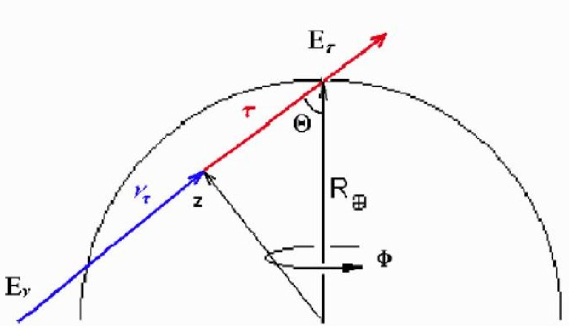
Figure 9: A neutrino $\nu_{\tau}$ crosses the Earth with energy $E_{\nu}$ at a nadir angle $\theta$ and azimuth angle $\phi$. Then it travels a distance $z$ before converting into a charged lepton $\tau$, which emerges from the Earth surface with energy $E_{\tau}$ [31].

This process can occur if and only if the following conditions are fulfilled:
a) the $\nu_{\tau}$ with energy $E_{\nu}$ has to survive along a distance $z$ through the Earth;
b) the neutrino converts into a $\tau$ in the interval $z,z+dz$;
c) the created lepton emerges from the Earth before decaying.

a) The probability $P_{a}$ that a neutrino with energy $E_{\nu}$ crossing the Earth survives up a certain distance $z$ is

$$P_{a}=\exp\left\{-\int_{0}^{z}\,\frac{dz^{\prime}}{\lambda_{CC}^{\nu}(E_{\nu},\,\theta,\,z^{\prime})}\right\}\,\,\,,$$ (5.10)

where

$$\lambda_{CC}^{\nu}(E_{\nu},\,\theta,\,z)=\frac{1}{\sigma_{CC}^{\nu N}(E_{\nu})\,\varrho[r(\theta,\,z)]\,N_{A}}$$ (5.11)

is the CC interaction length in the rock, $\varrho[r(\theta,\,z)]$ is the Earth’s density at distance $r$. The distance $r$ is given by $r^{2}(\theta,\,z)=R_{\oplus}^{2}+z^{2}-2{R_{\oplus}}z\cos\theta$, where $R_{\oplus}\simeq 6370\,\mathrm{km}$ is the average Earth radius. The expression of $P_{a}$ does not take into account the atmosphere crossed by the $\nu_{\tau}$ before entering the Earth surface, because the CC interaction length in the air is almost three orders of magnitude larger than in the rock.

b) The probability for $\nu_{\tau}\rightarrow\tau$ conversion in the interval $[z,\,z+dz]$ is

$$P_{b}=\frac{dz}{\lambda_{CC}^{\nu}\,(E_{\nu},\,\theta;\,z)}\,\,\,.$$ (5.12)

Here a comment is in turn. In order to produce a $\tau$ emerging with enough energy to generate a electromagnetic shower detectable by FD, the charged lepton propagation in the rock is limited. Moreover, since an EeV neutrino has a $\lambda_{CC}^{\nu}\sim 500$ km, only quite horizontal $\nu_{\tau}$ will be able to produce detectable events. The charged current interaction will then take place near to the Earth surface where the average density is almost constant and equal to $\varrho_{s}\simeq 2.65$ g/cm³.

c) The probability $P_{c}$ that a charged lepton loosing energy survives as it travels through the Earth is described by the coupled differential equations:

$$\frac{dP_{c}}{dz} = -\frac{m_{\tau}}{c\,\tau_{\tau}\,E_{\tau}}\,P_{c}\,\,\,,$$ (5.13)

$$\frac{dE_{\tau}}{dz} = -\left(\beta_{\tau}+\gamma_{\tau}\,E_{\tau}\right)\,E_{\tau}\,\varrho_{s}\,\,\,.$$ (5.14)

Here $m_{\tau}=1.8{\cdot}10^{9}$ eV, $\tau_{\tau}\simeq 3.4{\cdot}10^{-13}\,$s denotes the $\tau$ mean lifetime, whereas the parameters $\beta_{\tau}\simeq 0.71{\cdot}10^{-6}$ cm² g^-1 and $\gamma_{\tau}\simeq 0.35{\cdot}10^{-18}$ cm² g^-1 GeV^-1, as discussed in Section 4, fairly describe the $\tau$ energy loss in matter. The set of equations (5.13), (5.14) can be solved by observing that, following the results presented in section 3 and shown in Table 1, the tau lepton produced at $z$ carries an average energy which is a function of $E_{\nu}$. Let $E^{0}_{\tau}=E^{0}_{\tau}(E_{\nu})=(1-<y_{CC}>)E_{\nu}$ be the transferred energy. By solving Eq.s (5.13) and (5.14) at the emerging point on the Earth surface one has:

$$P_{c} = \left(F(E_{\nu},E_{\tau})\right)^{\omega}\,\exp\left\{-\frac{m_{\tau}}{c\tau_{\tau}\beta_{\tau}\varrho_{s}}\left(\frac{1}{E_{\tau}}-\frac{1}{E_{\tau}^{0}(E_{\nu})}\right)\right\}\,\,\,,$$ (5.15)

$$E_{\tau} = \frac{\beta_{\tau}\,E^{0}_{\tau}(E_{\nu})\,\exp\left\{-\varrho_{s}\,\beta_{\tau}(2R_{\oplus}\cos\theta-z)\right\}}{\beta_{\tau}+\gamma_{\tau}\,E^{0}_{\tau}(E_{\nu})\left(1-\exp\left\{-\varrho_{s}\,\beta_{\tau}(2R_{\oplus}\cos\theta-z)\right\}\right)}\,\,\,,$$ (5.16)

where

$$F(E_{\nu},E_{\tau})\equiv\frac{E^{0}_{\tau}(E_{\nu})(\beta_{\tau}+\gamma_{\tau}E_{\tau})}{E_{\tau}(\beta_{\tau}+\gamma_{\tau}\,E^{0}_{\tau}(E_{\nu}))}\,\,\,,\,\,\,\,\,\,\,\,\,\omega\equiv\frac{m_{\tau}\,\gamma_{\tau}}{c\tau_{\tau}\beta_{\tau}^{2}\varrho_{s}}\,\,\,.$$ (5.17)

The above results improve the ones obtained in Ref. [31], where a simpler parametrization for the $\tau$ energy loss was adopted.

The energy $E_{\tau}$ of the exiting lepton must be consistent with Eq.(5.16). This condition is enforced by the $\delta$-function:

$$P_{d}=\delta\left(E_{\tau}-\frac{\beta_{\tau}\,E^{0}_{\tau}(E_{\nu})\,\exp\left\{-\varrho_{s}\,\beta_{\tau}(2R_{\oplus}\cos\theta-z)\right\}}{\beta_{\tau}+\gamma_{\tau}\,E^{0}_{\tau}(E_{\nu})\left(1-\exp\left\{-\varrho_{s}\,\beta_{\tau}(2R_{\oplus}\cos\theta-z)\right\}\right)}\right)\,\,\,.$$ (5.18)

By using the expressions for the different probabilities (5.10), (5.12), (5.15), and (5.18) the kernel reads

$$K(E_{\nu},\,\theta;\,E_{\tau})=\int_{0}^{2R_{\oplus}\cos\theta}\,P_{a}\,P_{b}\,P_{c}\,P_{d}\,\,dz\,\,\,.$$ (5.19)

Once the integration over $z$ is performed, one gets the simple result

$$K(E_{\nu},\,\theta;\,E_{\tau})=\frac{\sigma_{CC}^{\nu N}(E_{\nu})\,N_{A}}{E_{\tau}(\beta_{\tau}+\gamma_{\tau}\,E_{\tau})}\,\left(F(E_{\nu},E_{\tau})\right)^{\xi}\,$$

$${\times}\exp\left\{-\frac{m_{\tau}}{c\tau_{\tau}\beta_{\tau}\varrho_{s}}\left(\frac{1}{E_{\tau}}-\frac{1}{E_{\tau}^{0}(E_{\nu})}\right)-2R_{\oplus}\cos{\theta}\,\sigma_{CC}^{\nu N}(E_{\nu})\,\varrho_{s}\,N_{A}\right\}\,\,\,,$$ (5.20)

where

$$\xi\equiv\left(\omega+\frac{\sigma_{CC}^{\nu N}(E_{\nu})\,N_{A}}{\beta_{\tau}}\right)\,\,\,.$$ (5.21)

Eq.(5.18) requires that two conditions are fulfilled. The first one is $E^{0}_{\tau}(E_{\nu})\geq E_{\tau}$ (obviously verified), while the second is

$$\cos\theta\geq\cos\theta_{min}=\frac{1}{2\,R_{\oplus}\,\beta_{\tau}\,\varrho_{s}}\,\log\left(F(E_{\nu},E_{\tau})\right)\,\,\,.$$ (5.22)

The expression (5.20) for the kernel $K(E_{\nu},\,\theta;\,E_{\tau})$ leads to the total rate of upgoing $\tau$’s showering on the Auger detector, and thus potentially detectable by the FD:

$$\frac{d\textsl{N}_{\tau}}{dt} = 2\pi S\,D\,\int_{E_{\nu}^{min}}^{E_{\nu}^{max}}dE_{\nu}\int_{E_{\tau}^{th}}^{E_{\tau}^{0}(E_{\nu})}dE_{\tau}\int_{\cos\theta_{min}}^{1}\,\frac{d\Phi_{\nu}(E_{\nu})}{dE_{\nu}\,d\Omega}\,$$ (5.23)

$${\times} K(E_{\nu},\,\theta;\,E_{\tau})\,\left(1-\exp\left\{-\frac{H\,m_{\tau}}{c\tau_{\tau}\,E_{\tau}}\right\}\right)\,\varepsilon\,\cos\theta\,d(\cos\theta)\,\,\,,$$

where we have used the isotropy of the considered neutrino flux. In Eq.(5.23) the quantity $S=3000\,\mathrm{km}^{2}$ is the geometrical area covered by the Auger apparatus, $D\sim 10\%$ is the duty cycle for fluorescence detection, $E_{\tau}^{th}\simeq 10^{18}$ eV is the energy threshold for the fluorescence process, and $E_{\nu}^{min}$ is the minimum neutrino energy capable of producing a $\tau$ at detection threshold. The quantity $E_{\nu}^{max}$ is the endpoint of the neutrino flux.

The exponential term in the r.h.s. of Eq.(5.23) accounts for the decay probability of a $\tau$ (showering probability) in a distance $H$ from the emerging point on the Earth surface. A detailed calculation of the fraction of Earth–skimming $\tau$’s decaying inside the fiducial volume would require a full Monte Carlo simulation, which is not the aim of the present analysis. A reasonable way to estimate such a fraction is to require that $\tau$ leptons travel a distance less than $H$ before decaying. We choose for simplicity $H=30$ km, which is the radius of an emisphere approximatively containing the entire PAO apparatus. However, this ansatz provides a conservative estimate of the number of events. FD detection efficiency $\varepsilon$ has been taken by Ref. [8].

In Eq.(5.23) the integration over $\cos\theta$ can be easily performed and this yields to

$$\frac{d\textsl{N}_{\tau}}{dt}=D\,\int_{E_{\nu}^{min}}^{E_{\nu}^{max}}dE_{\nu}\,\frac{d\Phi_{\nu}(E_{\nu})}{dE_{\nu}\,d\Omega}\,A(E_{\nu})\,\,\,,$$ (5.24)

where the effective aperture of the apparatus is here defined as

$$A(E_{\nu})=\frac{\pi S}{2\,R_{\oplus}^{2}\,N_{A}\,\varrho_{s}^{2}}\,\int_{E_{\tau}^{th}}^{E_{\tau}^{0}(E_{\nu})}dE_{\tau}\,\frac{\left(F(E_{\nu},E_{\tau})\right)^{\omega}}{E_{\tau}(\beta_{\tau}+\gamma_{\tau}\,E_{\tau})}\,$$

$${\times}\exp\left\{-\frac{m_{\tau}}{c\tau_{\tau}\beta_{\tau}\varrho_{s}}\left(\frac{1}{E_{\tau}}-\frac{1}{E_{\tau}^{0}(E_{\nu})}\right)\right\}\,\left(1-\exp\left\{-\frac{H\,m_{\tau}}{c\tau_{\tau}\,E_{\tau}}\right\}\right)\,\varepsilon$$

$${\times}\frac{1}{\sigma_{CC}^{\nu N}}\,\left[\left(1+\frac{\sigma_{CC}^{\nu N}\,N_{A}}{\beta_{\tau}}\log\left(F(E_{\nu},E_{\tau})\right)\right)\right.$$

$$-\left.\left(1+2\,R_{\oplus}\,\sigma_{CC}^{\nu N}\,\varrho_{s}\,N_{A}\right)\exp\left\{-2\,R_{\oplus}\,\sigma_{CC}^{\nu N}\,\varrho_{s}\,N_{A}\right\}\,\left(F(E_{\nu},E_{\tau})\right)^{\sigma_{CC}^{\nu N}N_{A}/\beta_{\tau}}\right].\,\,\,\,\,$$ (5.25)

Figure 10: The effective aperture, $A(E_{\nu})$, as defined in Eq.(5.25) is here plotted for $E^{th}_{\tau}=10^{17}$ eV and $H=30$ km, and for $E^{th}_{\tau}=10^{18}$ eV with $H=20$, 30, and 40 km, respectively.

In Figure 10 the quantity $A(E_{\nu})$ is plotted versus the neutrino energy for $E^{th}_{\tau}=10^{17}$ eV and $H=30$ km, and for $E^{th}_{\tau}=10^{18}$ eV with $H=20$, 30, and 40 km, respectively. The aperture for $E^{th}_{\tau}=10^{18}$ eV shows a maximum near $E_{\nu}\sim 10^{19}\,$ eV, sensibly dependent on the parameter $H$. For a lower energy threshold, for example $10^{17}$ eV, $A(E_{\nu})$ would scale as shown in Figure 10.

A similar analysis for the PAO Surface Detector has been performed via a Monte Carlo simulation in Ref. [32]. In particular, one could compare the aperture given in Figure 10 with Figure 9 of Ref. [32]. A direct comparison of the two calculations is difficult to be performed since the detector efficiency and the energy threshold of FD and SD differ. In our analysis we use an energy threshold $E^{th}_{\tau}=10^{18}$ eV. However, $A(E_{\nu})$ approaches the aperture of Ref. [32] as $E^{th}_{\tau}$ decreases.

In Table 2 the number of $\tau$-shower Earth–skimming events expected per year at the FD detector is reported for the models of neutrino flux discussed in section 2.

$dN_{\tau}/dt$ at FD	GZK-WB	GZK-L	GZK-H	TD	NH
# of UP events/year	0.02	0.04	0.09	0.11	0.25

Table 2: Yearly rate of upgoing (UP) events at FD for different neutrino models given in Figures 1 and 2.

In Ref. [31] an explicit plot of the aperture as defined in our Eq.(5.25) is not given. However, it is worth observing that the number of events reported in Table 2 for TD model is in fair agreement with the corresponding result of Ref. [31], once properly normalized to PAO effective area. Other cases are not immediately comparable since fluxes are different.

Figure 11: The quantity $dN_{\tau}/dE_{\tau}\,dt$ is plotted for the different neutrino models reported in Figures 1 and 2.

In Figure 11 the energy spectra of Earth–skimming events at FD are shown for the neutrino models of Figures 1 and 2. As expected, the maximum number of events is reached near to the assumed FD threshold ($\simeq$ 1 EeV), even though the maxima of neutrino fluxes are at higher energy. This can be easily understood by observing that tau leptons emerging inside the Auger surface with large energy and almost horizontally will probably decay far from the apparatus and are thus undetectable by the FD.

Figure 12: The most likely exit angle with respect to the horizontal for the emerging $\tau$ is plotted versus the energy of the primary neutrino.

By using the integrand in the r.h.s. of Eq.(5.24), the angle with respect to the horizontal of the Earth-skimming event $\alpha_{max}=\theta_{max}-\pi/2$ can be determined. Here, $\theta_{max}$ denotes the nadir angle for which the kernel of Eq.(5.24) has the maximum. This quantity is a function of neutrino energy via $\sigma_{CC}^{\nu N}$ and is shown in Figure 12.

As pointed out for example in Ref. [28], $\nu_{\tau}$ crossing deeply the Earth could experience a regeneration phenomenon which would eventually let $\tau$’s propagate up to the detector(see Figure 13). Furthermore, this process would also lead to the production at the CC vertex of secondary electron or muon neutrinos, then decaying in electrons or muons.

The contribution of regenerated $\nu_{\tau}$’s to the Earth–skimming event rate is negligible, since the process shown in Figure 13 is a second order transition in the weak coupling constant. Moreover, for $E_{\tau}^{th}\geq 5\cdot 10^{17}$ eV the Earth strongly suppresses the expected signal due to $\tau$ energy losses [25, 29]. As shown in Ref. [25, 29], the value of $E_{\tau}^{th}$ plays a crucial role in the estimate of the regenerated neutrino event rate, which results negligible for threshold energies larger than $10^{18}$ eV. Higher order processes including NC interactions, would also give negligible modifications to the numbers presented in Table 2. Finally, the associated secondary electron and muon neutrino flux does not enhance the Earth–skimming signal at PAO, since the charged leptons they produce are either absorbed or not detectable by FD.

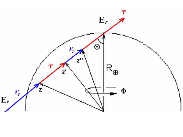
Figure 13: Second order regeneration process for $\nu_{\tau}$.

As well known, neutrino induced extensive air showers (see Ref. [63] for an extended discussion) can be disentangled by the ordinary cosmic ray background only for very inclined and deep showers. An estimate of the expected number of downgoing events (DW) within 30 km from the FD detector is given in Table 3 for different fluxes and increasing zenith angle. The DW event rates result to be comparable with the Earth–skimming ones of Table 2. As a final remark, the DW and Earth–skimming event rates are both affected by the uncertainty on the $\nu$-nucleon cross section, but, unlike the DW events, the Earth-skimming rate is also affected by the uncertainty on the tau energy losses in rock.

	GZK-WB	GZK-L	GZK-H	TD	NH
# of DW events/year ($\geq 60^{\circ}$)	$0.04$	$0.08$	$0.22$	$0.25$	$0.54$
# of DW events/year ($\geq 70^{\circ}$)	$0.02$	$0.04$	$0.10$	$0.12$	$0.25$
# of DW events/year ($\geq 80^{\circ}$)	$0.005$	$0.01$	$0.03$	$0.03$	$0.07$

Table 3: In the table are reported the expected number of downgoing events (DW) within 30 km from the FD detector for different fluxes and increasing zenith angle.

6 Conclusions

Ultra High Energy $\nu_{\tau}$’s ($E_{\nu}\geq 1\,EeV$) could have real detection chance at giant surface apparatus like PAO. Almost horizontal tau neutrinos crossing distance in the Earth of the order of their interaction length might produce $\tau$-shower Earth–skimming events potentially detectable by the Auger FD.

In this paper for a representative sample of $\nu_{\tau}$ fluxes either produced as cosmogenic neutrinos or in more exotic scenarios, the number of $\tau$-shower Earth–skimming events per year expected at the FD of the Pierre Auger Observatory has been computed. For this calculation we have used the CTEQ6 [33] parton distribution functions in the DIS factorization scheme and recent estimate of radiative $\tau$ energy losses in matter. A decrease of $\sigma_{CC}^{\nu N}$ allows $\tau$ to emerge with a smaller nadir angle (less horizontal) and thus increases the number of Earth–skimming events. In the relevant region of $E_{\nu}$, we essentially have $dN_{\tau}/dt\propto(\sigma_{CC}^{\nu N})^{-1}$; thus a factor $1/2$ in the neutrino-nucleon cross section leads to an almost double number of events at FD. As a further remark, we point out that the level of theoretical uncertainties on cross-sections at extremely high energy is very large (like in case of new physics above the TeV energy region), due to the poor experimental knowledge of parton density functions for very small $x$.

The number of events per year at the FD of the Pierre Auger Observatory is presented in Table 2 for the different neutrino models reported in Figure 1 and 2. For a five years PAO detection campaign (South plus North) we essentially have to scale these numbers by a factor ten and thus at least the exotic models could produce detectable events. However, it is worth noticing that this estimate has been performed under a rather conservative assumption on the possibility of $\tau$ showering on the apparatus: we have used an average value for the parameter $H$ which essentially allows only one particle out of three to decay inside the detection fiducial volume. In a paper in progress a more sophisticated simulation is going to be performed by taking into account the real morphology of the PAO site. This analysis should slightly increase the numbers presented in Table 2, which however give a reasonable estimate of the number of events at FD.

References

- [1] J. Linsley, Phys. Rev. Lett. 10 (1963) 146; Proc. 8th ICRC 4 (1963) 295.
- [2] See e.g. M.A. Lawrence, R.J. Reid and A.A. Watson, J. Phys. G 17 (1991) 733, and references therein.
- [3] D.J. Bird et al., Phys. Rev. Lett. 71 (1993) 3401; Astrophys. J. 424 (1994) 491; ibid. 441 (1995) 144.
- [4] N.N. Efimov et al., Proc. International Symposium on Astrophysical Aspects of the Most Energetic Cosmic Rays, eds. M. Nagano and F. Takahara (World Scientific Singapore, 1991) p.20; B.N. Afnasiev, Proc. of the International Symposium on Extremely High Energy Cosmic Rays: Astrophysics and Future Observatories, ed. M. Nagano (Institute for Cosmic Ray Research, Tokyo, 1996), p.32.
- [5] M. Takeda et al., Phys. Rev. Lett. 81 (1998) 1163; N. Hayashida et al., Astrophys. J. 522 (1999) 225. For general information see http ://www-akeno.icrr.u-tokyo.ac.jp/AGASA/.
- [6] D. Kieda et al., Proc. of the 26th ICRC, Salt Lake, 1999; T. Abu-Zayyad et al., HiRes Collaboration, astro-ph/0208243. For general information see http ://www.physics.utah.edu/Resrch.html.
- [7] P. Gorham et al. (ANITA Collaboration), http://www.ps.uci.edu/ barwick/anitaprop.pdf.
- [8] Auger Collaboration, The Pierre Auger Project Design Report, FERMILAB-PUB-96-024.
- [9] EUSO Collaboration, for general information see http://www.euso-mission.org.
- [10] C. Spiering et al. [BAIKAL Collaboration], astro-ph/0404096.
- [11] P. Niessen [AMANDA Collaboration], astro-ph/0306209.
- [12] F. Halzen, Am. Astron. Soc. Meeting 192, #62 28 (1998).
- [13] I. Kravchenko, astro-ph/0306408.
- [14] T. Montaruli et al. [ANTARES Collaboration], physics/0306057.
- [15] NEMO Collaboration, for general information see http://nemoweb.lns.infn.it.
- [16] NESTOR Collaboration, for general information see http://www.nestor.org.gr .
- [17] V. S. Beresinsky and G. T. Zatsepin, Phys. Lett. B 28, 423 (1969); V. S. Berezinsky and G. T. Zatsepin, Sov. J. Nucl. Phys. 11 (1970) 111 [Yad. Fiz. 11 (1970) 200].
- [18] P. Sreekumar et al., Astrophys. J. 494, 523 (1998) [astro-ph/9709257]; A. W. Strong, I. V. Moskalenko and O. Reimer, astro-ph/0306345; astro-ph/0405441.
- [19] O. E. Kalashev, V. A. Kuzmin, D. V. Semikoz and G. Sigl, Phys. Rev. D 66, 063004 (2002).
- [20] D. V. Semikoz and G. Sigl, JCAP 0404, 003 (2004).
- [21] K. S. Capelle, J. W. Cronin, G. Parente and E. Zas, Astropart. Phys. 8, 321 (1998) [arXiv:astro-ph/9801313].
- [22] F. Halzen and D. Saltzberg, Phys. Rev. Lett. 81, 4305 (1998).
- [23] D. Fargion, A. Aiello and R. Conversano, arXiv:astro-ph/9906450.
- [24] D. Fargion, Astrophys. J. 570, 909 (2002) [arXiv:astro-ph/0002453].
- [25] F. Becattini and S. Bottai, Astropart. Phys. 15, 323 (2001).
- [26] S. I. Dutta, M. H. Reno, I. Sarcevic and D. Seckel, Phys. Rev. D 63, 094020 (2001).
- [27] S. I. Dutta, M. H. Reno and I. Sarcevic, Phys. Rev. D 66, 077302 (2002).
- [28] J. F. Beacom, P. Crotty and E. W. Kolb, Phys. Rev. D 66, 021302 (2002).
- [29] S. Bottai and S. Giurgola, Astropart. Phys. 18, 539 (2003) [arXiv:astro-ph/0205325].
- [30] A. Kusenko and T. J. Weiler, Phys. Rev. Lett. 88, 161101 (2002).
- [31] J. L. Feng, P. Fisher, F. Wilczek and T. M. Yu, Phys. Rev. Lett. 88, 161102 (2002).
- [32] X. Bertou, P. Billoir, O. Deligny, C. Lachaud and A. Letessier-Selvon, Astropart. Phys. 17, 183 (2002).
- [33] http://user.pa.msu.edu/wkt/cteq/cteq6/cteq6pdf.html. See also: J. Pumplin et al. hep-ph/0201195, D. Stump et al. hep-ph/0303013.
- [34] E. V. Bugaev, Yu. V. Shlepin, Phys. Rev. D 67, 034027 (2003). See also hep-ph/0203096 v5.
- [35] V. S. Berezinsky and A. Yu. Smirnov, Ap. Sp. Sci. 32, 461 (1975).
- [36] E. Waxman and J. N. Bahcall, Phys. Rev. D 59, 023002 (1999) [hep-ph/9807282].
- [37] O. E. Kalashev, V. A. Kuzmin and D. V. Semikoz, astro-ph/9911035; Mod. Phys. Lett. A 16, 2505 (2001) [astro-ph/0006349].
- [38] M. Kachelriess, D. V. Semikoz and M. A. Tortola, Phys. Rev. D 68, 043005 (2003) [hep-ph/0302161].
- [39] P. Bhattacharjee and G. Sigl, Phys. Rept. 327, 109 (2000) [astro-ph/9811011].
- [40] N. G. Lehtinen, P. W. Gorham, A. R. Jacobson and R. A. Roussel-Dupre, Phys. Rev. D 69, 013008 (2004) [astro-ph/0309656].
- [41] P. W. Gorham, C. L. Hebert, K. M. Liewer, C. J. Naudet, D. Saltzberg and D. Williams, astro-ph/0310232.
- [42] S. Hannestad, JCAP 0305, 004 (2003) [arXiv:astro-ph/0303076].
- [43] P. Crotty, J. Lesgourgues and S. Pastor, Phys. Rev. D 69 (2004) 123007 [arXiv:hep-ph/0402049].
- [44] G. L. Fogli, E. Lisi, A. Marrone, A. Melchiorri, A. Palazzo, P. Serra and J. Silk, arXiv:hep-ph/0408045.
- [45] R. Gandhi, C. Quigg, M. Reno, I. Sarcevic, Phys. Rev. D 58, 093009 (1998).
- [46] V. N. Gribov and L. N. Lipatov, Yad. Fiz. 15, 1218 (1972) [Sov. J. Nucl. Phys. 15, 675 (1972)].
- [47] L. N. Lipatov, Sov. J. Nucl. Phys. 20, 94 (1975) [Yad. Fiz. 20, 181 (1974)].
- [48] Y. L. Dokshitzer, Sov. Phys. JETP 46, 641 (1977) [Zh. Eksp. Teor. Fiz. 73, 1216 (1977)].
- [49] G. Altarelli and G. Parisi, Nucl. Phys. B 126, 298 (1977).
- [50] S. I. Dutta, M. H. Reno, I. Sarcevic, Phys. Rev. D 63, 094020 (2001).
- [51] S. R. Kelner, V. V. Kotov, Sov. J. Nucl. Phys. 7, 237 (1968).
- [52] R. P. Kokoulin, A. A. Petrukhin, Proc. of Int. Cosmic Ray Conf. (ICRC 71), Hobart 6, A2436 (1971).
- [53] Yu. M. Andreev, E. V. Bugaev, Phys. Rev. D 55, 1233 (1997).
- [54] S. Bottai, L. Perrone, Nucl. Instr. and. Meth. A 459, 319 (2001).
- [55] W. Lohmann, R. Kopp, R. Voss, CERN yellow report 85-03 (1985).
- [56] I. A. Sokalski, E. V. Bugaev, S. I. Klimushin, Phys. Rev. D 64, 074015 (2001).
- [57] L. B. Bezrukov, E. V. Bugaev, Sov. J. Nucl. Phys. 33, 635 (1981).
- [58] E. Bugaev, T. Montaruli, Y. Shlepin, I. Sokalski, hep-ph/0312295 v2.
- [59] M. Derrick et al. [ZEUS Collaboration], Phys. Lett. B 293, 465 (1992).
- [60] T. Ahmed et al. [H1 Collaboration], Phys. Lett. B 299, 374 (1993).
- [61] P. Lipari and T. Stanev, Phys. Rev. D 44, 3543 (1991).
- [62] S. Bottai and S. Giurgola, Astropart. Phys. 18, 539 (2003).
- [63] M. Ambrosio, C. Aramo, A. Della Selva, G. Miele, S. Pastor, O. Pisanti and L. Rosa, arXiv:astro-ph/0302602.