Improving XMM–Newton EPIC pn data at low energies:
method and application to the Vela SNR

Abstract

High quantum efficiency over a broad spectral range is one of the main properties of the EPIC pn camera on–board XMM-Newton. The quantum efficiency rises from $\sim 75\,\%$ at 0.2 keV to $\sim 100\,\%$ at 1 keV, stays close to 100 % until 8 keV, and is still $\sim 90\,\%$ at 10 keV [1]. The EPIC pn camera is attached to an X–ray telescope which has the highest collecting area currently available, in particular at low energies (more than 1400 cm² between 0.1 and 2.0 keV)[2]. Thus, this instrument is very sensitive to the low–energy X–ray emission. However, X–ray data at energies below $\sim 0.2\mbox{ keV}$ are considerably affected by detector effects, which become more and more important towards the lowest transmitted energies. In addition to that, pixels which have received incorrect offsets during the calculation of the offset map at the beginning of each observation, show up as bright patches in low–energy images. Here we describe a method which is not only capable of suppressing the contaminations found at low energies, but which also improves the data quality throughout the whole EPIC pn spectral range. This method is then applied to data from the Vela supernova remnant.

1 INTRODUCTION

The EPIC pn camera on–board XMM–Newton is currently the most sensitive instrument in space for detecting soft X–rays. In order to fully utilize this unique capability, we have developed methods which improve the data quality in particular at low energies. These methods are generally available in SASS v6.0, the most recent version of the XMM–Newton Science Analysis System, in the task epreject.

In Section 2 we describe a method which removes bright patches that become visible in low–energy images. This is achieved by correcting the energy of events which are detected in the corresponding pixels. Thus, this method does not only improve the cosmetic quality of low–energy images, but does also improve the spectral quality thoughout the whole bandpass of EPIC pn. Although the most straightforward application of this method requires the presence of the offset map for the corresponding exposure, we have extended this method so that it can also be applied if only the event file is available.

Another improvement, described in Section 3, concerns the suppression of detector noise, which becomes significant at energies below $\sim 200\mbox{ eV}$. This is done by computing the probability that a specific event may be a noise event and by assigning, on a statistical basis, appropriate flags to individual events. Subsequent removal of events which were flagged as due to detector noise leads to a conspicuous improvement of the data quality below $\sim 300\mbox{ eV}$ and makes the background subtraction in this energy range more reliable. Additionally, as a by–product, the event files become considerably smaller and easier to handle.

In Section 4, we demonstrate these methods on the example of an XMM EPIC pn observation of an area within the Vela supernova remnant. In particular we show how the noise suppression method reveals the presence of soft diffuse emission at energies below $\sim 200\mbox{ eV}$ which would otherwise be hidden in the detector noise.

2 OFFSET SHIFTS

2.1 The Problem

The usual mode of operating the EPIC pn camera consists of taking an offset map immediately before the beginning of an exposure. Ideally, this map contains for each pixel the energy offset (expressed in analog–to–digital units, adu). During the subsequent exposure, these offsets are subtracted on–board from the measured signals, and only events where the difference signal exceeds a lower threshold (usually 20 adu) are transmitted to Earth.

The offset map is calculated in the following way: the charge in each pixel is read out one hundred times, the three smallest and the three highest adu values are ignored, and the sum of the remaining values, divided by 94 and truncated to the nearest integer, is computed as the offset of that pixel. This procedure is applied subsequently to regions of $64\times 4\mbox{ pixels}$ along each CCD. The reason for excluding the extreme values is to minimize the influence of energetic particles on the offset calculation. The highest adu values are ignored because the charge deposited by minimum ionizing particles is usually close to the upper end of the dynamic adu range. However, the charge deposited by a highly ionizing particle may show up as a very small charge, because the large amount of charge generated by such a particle takes a long time to be cleared from the anode. Depending on the number of signal electrons, the clearing goes on during the readout of the next pixels, and the measured adu value is thus slighly reduced. Therefore, also the smallest adu values are ignored.

Figure 1: Number of events per pixel and Ms ($=10^{6}\mbox{ s}$) as a function of raw pulse height amplitude [adu] for a $23.1\cdot 10^{3}\mbox{ s}$ exposure (obtained during revolution #462) in full frame mode with the filter wheel closed. These spectra are shown individually for all EPIC pn quadrants (arranged according to their position on the detector). Note the different intensity of detector noise in the four quadrants.

There are cases where so much charge is deposited by highly ionizing particles that it takes several frames until the original state is restored. It may also happen that several minimum ionizing particles are hitting the same pixels during the one hundred readouts. At such occasions the technique of rejecting the three smallest and the three highest adu values before computing the mean offset is not sufficient, and the offset is not computed correctly. As the erroneous adu values are predominantly too low, the computed mean offset becomes too small. This effect introduces in the affected pixels deviations from the correct offsets which range typically from $-5\mbox{ adu}$ to $+3\mbox{ adu}$, corresponding to energy shifts from $-25\mbox{ eV}$ to $+15\mbox{ eV}$. As a consequence, the energies of all events in these pixels appear to be shifted by the same amount. The number of affected pixels scales with the intensity of the particle background during the calculation of the offset map and depends also on the readout mode. From our analysis of full frame mode (FF) data, we find that 54% of all pixels contain correct offsets, while for 26% the offset is by 5 eV too high and for 12% it is by 5 eV too small. Deviations of this amount ($\pm 1\mbox{ adu}$) are not necessarily all caused by energetic particles, as they may also reflect statistical and numerical fluctuations in the computation of the offset map. Larger deviations, however, can clearly be attributed to energetic particles, as can be seen by their characteristic pattern (e.g. Fig. 2c). For 5% the offset is by 10 eV too high and for 2% it is by 10 eV too small. Offsets of 15 eV and more were found for 1% of the pixels. For $\sim 70\%$ of them, the offset was too small.

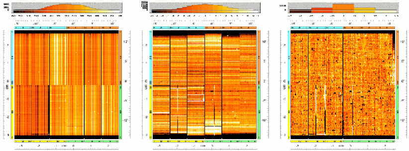
a                                                 b                                                 c

Figure 2: Computing the “residual offset map”: a) Original offset map for the observation 0526_0147511101. The vertical stripes are mainly caused by differences in the gain of the individual columns. b) Same as (a), but after subtracting from each column its median value. The horizontal stripes are mainly caused by the common mode effect (see Sect. 2.2.1). c) Same as (b), but after subtracting also from each row its median value. The remaining patterns in this “residual offset map” are a superposition of persistent features and temporary patches caused by energetic particles.

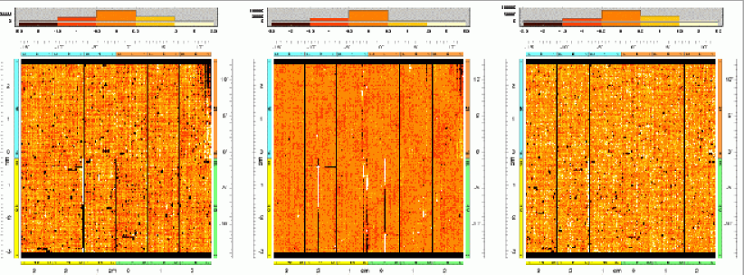
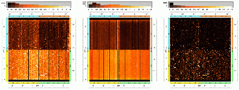
a                                                 b                                                 c a                                                 b                                                 c

Figure 3: Separating the persistent and temporary features in the residual offset map: a) Same as Fig. 2 c, but for a different observation (523_0147510801); note the different distribution of most patches. b) “Residual offset reference map”: this map shows for each pixel the median of seven residual offset maps (from revs 522, 523, 525, 526, 527, 528, and 544) and thus contains the persistent features in the residual offset maps. c) Difference (a) $-$ (b), containing the temporary features for this specific observation.

Figure 4: Separating the persistent and temporary features in the 20 adu image: a) Distribution of all events with 20 adu accumulated in the 76 ks observation 523_0147510801, normalized to 1 ks. b) “20 adu reference map”: this map shows for each pixel the median of ten residual offset maps (from revs 344, 349, 522, 523, 525, 526, 527, 528, 544, and 548), each normalized to 1 ks exposure, and thus contains the persistent features in the 20 adu maps. c) Difference (a) $-$ (b), containing the temporary features for this specific observation. Note the similarity with Fig. 4 c.

If the offset subtracted on–board was too small, then the adu values which are assigned to events in such pixels became too high. Thus, events which have adu values below the lower threshold and which would normally have been rejected, may show up in the data set. As most of such events are due to detector noise, which is steeply increasing towards lower energies (Fig. 1), any reduction of the lower energy threshold leads to a considerable increase in the number of events. Thus, pixels where the offset is too small show up as bright patches in images accumulated in the lowest transmitted adu range. Due to the specific pixel block sampling applied for the offset map calculation (see above), these patches appear as rectangular areas, which are characterized by a brightening in four consecutive pixels along readout direction. Depending on the width of the trail caused by the energetic particles and its orientation with respect to the CCD, the patches may also extend over several consecutive pixels perpendicularly to the readout direction. Pixels with too high offsets are less obvious in low–energy images, as they are only somewhat darker than their environment.

While the occurrence of bright patches in EPIC pn images which are accumulated at low energies (e.g. Fig. 4) is immediately obvious, there is also another consequence: a shift in the energy scale over the whole spectral bandpass. This shift degrades the energy resolution for extended objects. For point sources, the X–ray spectrum may be shifted by some 10 eV, in most cases towards higher energies, if the position of the source happens to coincide with one of these patches. Here we describe a method for restoring the correct energy scale and for removing the bright patches in the soft energy images. Although this paper concentrates on the low energy properties of EPIC pn data, we note that the correction of the offset shifts improves the energy calibration throughout the full spectral bandpass of the EPIC pn detector.

2.2 Correcting the energy scale

The correction is more straightforward if the offset map is available. If this is not the case, then the offsets have to be reconstructed from the spatial and spectral distribution of the transmitted events. These two cases are described in the next sections.

2.2.1 If the offset map is available

The offset map contains for each pixel the adu value which was subtracted from all events in the particular pixel before transmitting this information to ground. As it contains both correct and incorrect offsets, the main goal is to distinguish between both cases. Such a distinction is possible under the assumption that the generic offsets of all pixels (not affected by electronic effects during readout) are very similar and that the areas where incorrect offsets were computed occur in isolated patches.

The most obvious property of the offset map is a pattern of vertical stripes (Fig. 2a). This is caused by the fact that each of the 768 readout columns has its own amplifier, and the amplification varies by $\pm 4.1\%$ (rms) from column to column. In order to spot the patches where wrong offsets have been applied, the column to column variation has to be removed. This can be achieved by subtracting the median value from each column. The resulting map (Fig. 2b) is dominated by row to row variations, which are mainly caused by the “common mode” effect: a temporal change of the offsets of all the pixels in a CCD row, occurring in a predominantly irregular way. This effect is present during the calculation of the offset map as well as during the subsequent exposure. During the exposure, it is suppressed on–board by subtracting first the adu offsets contained in the offset map, and then the median of all the adu values in a CCD row from these values, individually for each readout frame. Concerning the further processing of the offset map, this implies that the median value of each row should also be subtracted from the corresponding row, in order to remove the row to row variation. This leads to a “residual offset map” (Fig. 2c), which is close to zero except for the pixels where specific offsets were applied.

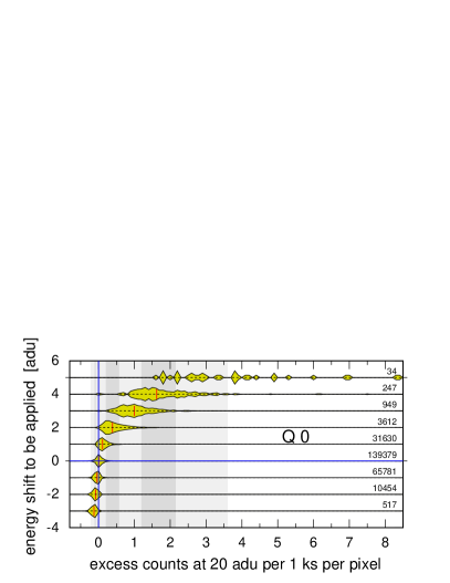
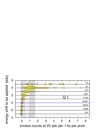
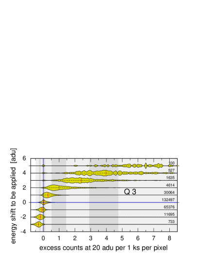
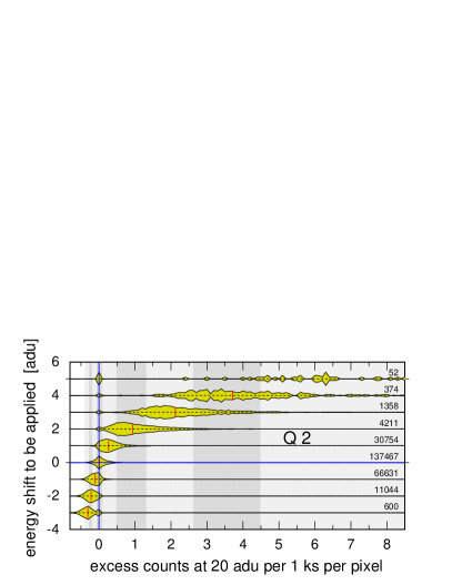
Figure 5: Pixel by pixel correlation between the excess counts at 20 adu, normalized to 1 ks, and the values in the cleaned offset map, for all quadrants (arranged according to their position on the detector). While the energy shifts to be applied can only occur as integer multiples of 1 adu ($\sim 5\mbox{ eV}$), the excess counts exhibit a much smoother distribution due to their normalization to 1 ks. Their distribution is illustrated by the thickness of “histogram tubes”, which were all expanded to have the same maximum thickness. The number of pixels which they contain are given at right. This correlation was derived by combining the observations of the Lockman hole in XMM revolutions 522, 523, 525, 526, 527, 528, and 544 ($\sim 636\mbox{ ks}$ total exposure time), all taken in fullframe mode. For Q 3, four noisy columns were excluded. A vertical red line indicates the median value of the distributions. Shaded areas show the ranges of excess counts for which a certain energy shift should be applied. Note how the brightness of pixels at 20 adu responds differently in the four quadrants to energy shifts. No such variation was found within the CCDs of the same quadrant.

Figure 6: Extrapolation of the empirical correlation between excess counts in the 20 adu image and the energy shift to be applied. The numbers below the horizontal steps specify the boundaries of the interval of excess counts, where the energy scale should be corrected by the adu values given to the left of the horizontal steps. The extrapolation was done by fitting a cubic function to the median values of the excess counts found for offset shifts between $-2$ and $+4\mbox{ adu}$ (cf. Fig. 5); these points are marked by small dots. An extrapolation was necessary because corrections by more than 4 adu may occur, but they do not occur frequently enough for a direct determination of the correlation function.

However, not all of the offsets in the residual offset map are artefacts caused by energetic particles. Comparison of such maps (e.g. Figs. 2c and 4a) indicates that they consist of a superposition of both persistent and temporally variable patterns. By computing for each pixel the median value of several such maps, only the persistent patterns remain (Fig. 4b). Subtraction of such a “residual offset reference map” from an individual residual offset map reveals then the temporally variable content of this “cleaned offset map”. Comparison of such maps with images accumulated from the low–energy events in the subsequent exposure (see Fig. 4a and Sect. 2.2.2) shows a clear correlation between the position of the bright patches in the low–energy image and the pixels which have a non–zero value in the cleaned offset map. This shows that the patches seen in the cleaned offset maps reflect incorrect offsets caused by energetic particles.

As the processed offset maps contain directly the adu shifts which have to be subtracted from all events in the corresponding pixels in order to reconstruct the correct energy scale, an implementation of this algorithm is straightforward. However, while the correct energy scale can be reconstructed, there is no possibility to recover events which were not transmitted to ground because a too high offset was subtracted so that they fell below the lower energy threshold. On the other hand, events where a too low offset was subtracted will show up after the correction with adu values below the lower threshold. In order to restore a homogeneous data set, these events should be removed afterwards. Then the gain and CTI correction should be repeated for the whole data set.

2.2.2 If the offset map is not available

Even if the offset map is not available (this was the general situation in the past), the correction described above can be achieved, by extracting the necessary information directly from the event file. This is possible because the amount of noise events is a monotonically and steeply increasing function towards lower energies (Fig. 1). As this function is also fairly stable in time, the intensity of a pixel in the lowermost energy channel transmitted (20 adu) is expected to be correlated with the shift in the energy scale: if the energy scale in a pixel is shifted by only 1 adu towards higher energies, i.e., if the 20 adu bin contains 19 adu events, then this pixel should contain $\sim 1.8$ times more events.

However, this correlation is disturbed by the fact that the brightness of a pixel at 20 adu is also influenced by other factors, in particular by its individual noise properties. In Fig. 4a, the lower half of the detector (Q 2 and Q 3) are brighter than the upper one (Q 0 and Q 1). Comparison with Fig. 1 shows that this behaviour is caused by the fact that there are more noise events at 20 adu in Q 2 and Q 3 than in Q 0 and Q 1. In addition to the brightness differences from quadrant to quadrant, brightness variations can also be seen within the quadrants and even within the CCDs (Fig. 4a).

Separation of brightness variations caused by shifts in the energy scale from variations caused by other effects can be achieved with a similar method as applied to the residual offset maps (Sect. 2.2.1): from a set of 20 adu images, derived from long exposures with no bright sources in the field of view and normalized to the same exposure time, a reference image can be computed, containing for each pixel the median value, i.e., its nominal, temporally constant, 20 adu brightness (Fig. 4b). This reference image can then be subtracted from an individual 20 adu image, in order to derive the brightness variations characteristic for that particular exposure. The resulting “cleaned 20 adu image” (Fig. 4c) shows a clear spatial correlation with the cleaned offset map of the same exposure (Fig. 4c). In addition to the spatial correlation, there is also a direct correlation between the brightness of the pixels in the cleaned 20 adu images (normalized to the same exposure time) and the cleaned offset maps, as expected. This correlation (Fig. 5) is different between the four quadrants, due to their different noise properties. No such differences were found among the CCDs within a quadrant.

The correlation shown in Fig. 5 was derived from seven long observations of the Lockman hole ($\sim 636\mbox{ ks}$ in total). This region contains only faint sources, which cannot disturb the offset maps or the 20 adu images. Due to the long exposure times, the statistical uncertainties in the number of excess counts at 20 adu are minimized. The statistical quality is good enough to deduce the energy shifts to be applied from the number of excess counts for the range from $-3$ to $+4\mbox{ adu}$. As larger shifts do not occur frequently enough for a direct determination of the correlation function, they were determined by extrapolation (Fig. 6).

With the correlation derived above, it becomes possible to reconstruct the offset shifts directly from the event file, at least in an approximate way: while offset shifts can occur only at discrete adu steps, the correspondence between the 20 adu brightness and the value of the offset shift is not always unique (Fig. 5). In addition, the presence of Poissonian noise in the 20 adu images, in particular for short exposures, limits the sensitivity for locating the pixels where a correction of the energy scale should be applied. The sensitivity of locating such pixels can be increased by rebinning four consecutive rows of the 20 adu image into one row each, in order to utilize the information about how the offset map was calculated on–board. Nevertheless, this method is less accurate than the technique described in the previous section, but it does improve the overall data quality and can be applied if no offset map is available.

Figure 7: Oblique view onto the EPIC pn detector, illustrating the spatial variations of detector noise for the fullframe mode. For each row of each CCD, the noise spectrum in the range 20 – 65 adu is displayed in a color code which extends from 0 (black) to 0.01 events ks^-1 px^-1 adu^-1 (white); the maximum value is 1.3 events ks^-1 px^-1 adu^-1. In order to cover the high dynamic range, the colors change with the square root of the noise. These spectra were derived from 10 exposures with the filter wheel closed (in XMM revolutions 129, 266, 339, 351, 363, 393, 409, 454, 462, 532), yielding a total exposure time of 144 ks. The information displayed here is used for the suppression of the detector noise.

3 DETECTOR NOISE

While there is practically no detector noise present at energies above $80\mbox{ adu}$ ($\sim 400\mbox{ eV}$), X-ray data below this energy, in particular below 40 adu ($\sim 200\mbox{ eV}$), are considerably contaminated by noise events, which become more and more dominant towards the lowest transmitted energy channels (Fig. 1). Investigations of 40 hours of in–orbit calibration data with the filter wheel closed, taken over a period of more than two years, show that the noise properties vary with position and energy, but are fairly stable in time for most areas on the detector. This property enables a statistical approach for suppressing the detector noise: with the information about the spatial and spectral dependence of the detector noise, the amount of events which correspond to the expected noise can be flagged and suppressed.

The noise properties were derived from 10 exposures in fullframe mode, with the filter wheel closed, between XMM–Newton revolutions #129 and #532, yielding a total exposure time of 144 ks. These measurements were first corrected for offset shifts (see Sect. 2) and then used for accumulating raw spectra below 65 adu, individually for each CCD row (Fig. 7). The fine spacing along readout direction was chosen because the noise properties change considerably with distance from the readout node, in particular close to the node. In order to get a sufficient number of events, no subdivision was made along the CCD rows. This approach was motivated by the fact that the noise properties do not show a pronounced dependence along this direction (unless there is a bright column). As the resulting spectra suffered somewhat from low count rate statistics, they were smoothed along readout direction with a running median filter extending over $\pm 5$ rows. This smoothing was not applied to the 20 rows closest to the readout nodes, where the spectra contained more counts and where the dependence of the spectra on the distance from the readout nodes is high.

With this information, potential noise events in a specific observation can be suppressed, on a statistical basis, in the following way: for each CCD row and adu bin, the number of events is compared with the corresponding value in the noise data (scaled to the same exposure). According to the ratio between the actual number of events and the expected noise contribution, individual events can then be randomly flagged. In order to improve the statistics somewhat, the spectra from the observation to be corrected are internally smoothed by a running median filter along readout direction before the noise contribution is computed.

This method extends the usable energy range down to the lowest energies transmitted, i.e. $\sim 120\,-\,140\mbox{ eV}$, depending on the position on the CCD. Below this energy, parts of the detector become essentially insensitive due to the low energy threshold applied on–board and the combined effect of charge transfer loss and gain variations within the 768 amplifiers in the EPIC pn camera. In addition to the improvement of the data quality, a removal of events which were flagged as noise events also makes the files considerably smaller and easier to handle.

Suppressing the detector noise by this method has not only advantages for images, but leads also to a more reliable subtraction of detector noise in the spectra and thus to an improved spectral quality. A large part of the instrumental background can be taken into account by the unusal technique of background subtraction, i.e., by determining the background spectrum from a different region on the detector and subtracting it, appropriately scaled, from the spectrum to be analysed. However, as the detector noise is not vignetted (in contrast to background coming through the X–ray telescope) and not distributed homogeneously across the detector (Fig. 7), the usual background subtraction technique may lead to a systematic error in the normalization of the low–energy part of the spectrum. Another interesting consequence of the noise suppression method described here for spectral studies is that the detector noise can be separated from other background components.

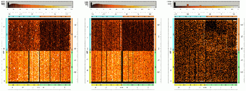
a                                                 b                                                 c

Figure 8: Illustration of the steps for correcting and cleaning the data set for the 33.0 ks observation of the Vela SNR in XMM rev. 367. Shown are images accumulated from all events in the lowest energy channel transmitted (20 adu). These images are dominated by detector noise (cf. Fig. 1), despite the presence of the SNR. a) Image derived from the original data set. b) Image after correcting the energy scale in specific pixels. c) Image after suppressing also the detector noise. Note the different color scale, which extends from 0 to 50 events per pixels for (a) and (b), but from 0 to 5 events per pixels for (c).

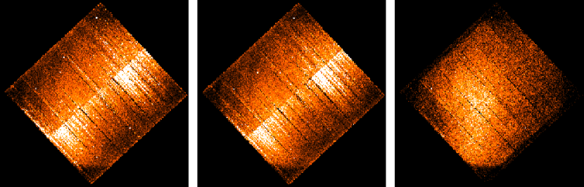
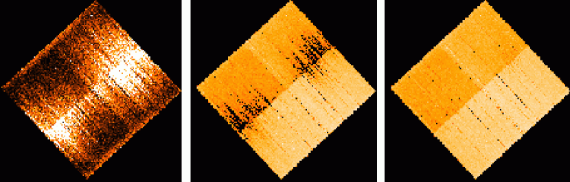
a                                                 b                                                 c a                                                 b                                                 c

Figure 9: Effects of the steps illustrated in Fig. 8 on a low–energy image of the Vela SNR. These image are all accumulated in celestial coordinates (cf. Fig. 12) in the (instrumental) energy range 120 –200 eV. a) Original image, b) after correcting the energy scale in specific pixels, c) after suppressing also the detector noise. The color scale extends from 0 to 40 events per pixel for (a) and (b), and from 0 to 20 events per pixel for (c). The original image (a) contains $1.4\cdot 10^{6}\mbox{ events}$, while the cleaned image (c) contains only $0.5\cdot 10^{6}\mbox{ events}$.

Figure 10: a) Events in the 120 – 200 eV energy range which were rejected as due to detector noise. The color scale extends from 0 to 20 events per pixel. This image contains $0.9\cdot 10^{6}\mbox{ events}$ in total. b) Image of all events with (instrumental) energies below 120 eV, after correcting the energy scale in specific pixels, and displayed in a logarithmic color scale extending from 0 to 500 events per pixel. This image shows that not all areas of the detector are sensitive to energies below 120 eV. c) Same as (b), but for energies below 140 eV. The insensitive areas have practically all disappeared.

4 APPLICATION TO THE VELA SNR

Here we apply the methods described in Sections 2 and 3 to a 33 ks observation of the Vela supernova remnant, performed in December 2001 (XMM rev. 367) in fullframe mode with the medium filter. The observed region (Fig. 12) contains the north–west rim of another supernova remnant, RXJ 0852.0-4622, which was discovered in the ROSAT all–sky survey[3]. Compared to the Vela SNR, which is $\sim 2\cdot 10^{4}\mbox{ years}$ old, RXJ 0852.0-4622 is considerably younger (less than $1.5\cdot 10^{3}\mbox{ years}$, with $\sim 680\mbox{ years}$ as the most probable value[4]) and is emitting more energetic X–rays. In the ROSAT data, it becomes visible only above 1.3 keV. At lower energies, it is outshone by the bright emission of the Vela SNR (Fig. 12).

Figure 8a shows the EPIC pn data of this observation accumulated at 20 adu, the lowest energies transmitted. White patches resulting from erroneous energy offsets are clearly seen. After applying the local corrections of the energy scale described in Section 2, these patches disappear (Fig. 8b). The data, however, are still dominated by detector noise. This noise can be suppressed by more than one order of magnitude at 20 adu (Fig. 8c) with the method described in Section 3.

Although the 20 adu images are well suited for performing and verifying the corrections, the spectral bandwidth is too small to see diffuse X–ray emission from the Vela region. In order to demonstrate the improvement in the low–energy X–ray data, Figs. 10 a-c show images for the 120 – 200 eV energy band, corresponding to the steps illustrated in Figs. 8 a-c, The cleaned image (Fig. 10c) reveals that there is indeed diffuse X–ray emission present, which is, however, lost in the detector noise if no correction is applied (Fig. 10a). The cleaning in this energy range is substantial: 2/3 of the original events at 120 –200 eV were suppressed as due to detector noise. Fig. 10a shows an image of all the events which were been removed, in the same intensity scale as Fig. 10c.

While these methods make it possible to extend the useful energy range down to $\sim 120\mbox{ eV}$, there is a constraint which cannot be avoided: the combined effects of charge transfer losses and variations in the gain of the 768 amplifiers cause an increase of the local low energy threshold (20 adu at readout, corresponding to an instrumental energy of 100 eV) for specific areas on the detector. This is illustrated in Fig. 10b, which demonstrates that not all areas of the detector are sensitive to energies below 120 eV. Homogeneous sensitivity across the whole detector is reached at energies above $\sim 140\mbox{ eV}$ (Fig. 10c).

All the images shown so far were obtained at energies below 200 eV. However, the improvement in data quality is not restricted to this energy range. Comparison of the spectra obtained before and after the correction (Fig. 12) indicates that the detector noise is suppressed up to $\sim 400\mbox{ eV}$ (corresponding to 80 adu), where it becomes negligible (cf. Fig. 1). The high sensitivity of XMM EPIC pn makes it possible to produce several narrow–band images of the Vela SNR region below 1 keV. Figure 13 shows exposure corrected images derived from the corrected and cleaned data set in the energy bands indicated in Fig. 12a. These images reveal a stunning variety of complex X–ray emission, which changes considerably with energy, even in this small 0.1 – 1. keV spectral range. Due to the improved spectral resolution of XMM compared to ROSAT, emission from the north–west rim of the young supernova remnant RXJ 0852.0-4622, which is visible in the ROSAT data only above 1.3 keV, is already obvious at energies above $\sim 0.7\mbox{ keV}$.

      Figure 11: ROSAT 0.1 – 0.4 keV image of the eastern part of the Vela SNR, obtained during the all–sky survey. The white contour outlines the XMM–Newton EPIC pn field of view during the observation in rev. 367 (cf. Fig. 13). Figure 12: EPIC pn spectra of the full field of view from the pointing to the Vela SNR, displayed in a linear (a) and logarithmic (b) scale. The spectra are composed of all “good” (FLAG = 0) and valid patterns (singles, doubles, triples, and quadruples). The upper curves show the original spectra, while the lower curves are the result of the corrections described in the text. Shaded areas in (a) mark the energy bands which were selected for creating the images in Fig. 13.

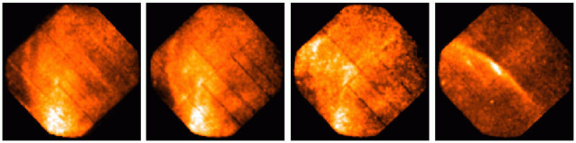
a) 140 – 200 eV b) 250 – 450 eV c) 500 – 650 eV d) 700 – 1100 eV

Figure 13: EPIC pn images of the region of the Vela SNR containing the north–west rim of RXJ 0852.0-4622, observed in XMM rev. 367 (cf. Fig. 12). The energy ranges indicated below each image are also shown in  Fig. 12a. All images have been corrected for exposure variations and are composed of all valid patterns, after having applied the processing steps described in the text. Note the pronounced changes of the X–ray appearance in this small region of the X–ray spectrum.

References

- [1] R. Hartmann, G. D. Hartner, U. G. Briel, K. Dennerl, F. Haberl, L. Strueder, J. Truemper, E. Bihler, E. Kendziorra, J. E. Hochedez, E. Jourdain, P. Dhez, P. Salvetat, J. M. Auerhammer, D. Schmitz, F. Scholze, and G. Ulm, “Quantum efficiency of the XMM pn-CCD camera,” in Proc. SPIE Vol. 3765, p. 703-713, EUV, X-Ray, and Gamma-Ray Instrumentation for Astronomy X, Oswald H. Siegmund; Kathryn A. Flanagan; Eds., pp. 703–713, Oct. 1999.
- [2] F. Jansen, D. Lumb, B. Altieri, J. Clavel, M. Ehle, C. Erd, C. Gabriel, M. Guainazzi, P. Gondoin, R. Much, R. Munoz, M. Santos, N. Schartel, D. Texier, and G. Vacanti, “XMM-Newton observatory. I. The spacecraft and operations,” A&A 365, pp. L1–L6, Jan. 2001.
- [3] B. Aschenbach, “Discovery of a young nearby supernova remnant,” Nature 396, pp. 141–142, 1998.
- [4] B. Aschenbach, A. F. Iyudin, and V. Schönfelder, “Constraints of age, distance and progenitor of the supernova remnant RXJ 0852-4622/GRO J0852-4642,” A&A 350, pp. 997–1006, 1999.