Origin of Tidal Dissipation in Jupiter: II. the Value of $Q$

Abstract

The process of tidal dissipation inside Jupiter is not yet understood. Its tidal quality factor ($Q$) is inferred to lie between $10^{5}$ and $10^{6}$. Having studied the structure and properties of inertial-modes in a neutrally buoyant, core-less, uniformly rotating sphere (Wu, 2004), we examine here their effects on tidal dissipation. The rate of dissipation caused by resonantly excited inertial-modes depends on the following three parameters: how well they are coupled to the tidal potential, how strongly they are dissipated (by the turbulent viscosity), and how densely distributed they are in frequency. We find that as a function of tidal frequency, the $Q$ value exhibits large fluctuations, with its maximum value set by the group of inertial-modes that satisfy $\delta\omega\sim\gamma$, where $\delta\omega$ is the group’s typical offset from an exact resonance, and $\gamma$ their turbulent damping rates. These are intermediate order inertial-modes with wave-number $\lambda\sim 60$ and they are excited to a small surface displacement amplitude of order $10^{3}\,\rm cm$. The $Q$ value drops much below the maximum value whenever a lower order mode happens to be in resonance. In our model, inertial-modes shed their tidally acquired energy very close to the surface within a narrow latitudinal zone (the ’singularity belt’), and the tidal luminosity escapes freely out of the planet.

Strength of coupling between the tidal potential and inertial-modes is sensitive to the presence of density discontinuities inside Jupiter. In the case of a discreet density jump, as may be caused by the transition between metallic and molecular hydrogen, we find a time-averaged $Q\sim 10^{7}$, with a small but non-negligible chance ($\sim 10\%$) that the current $Q$ value falls within the empirically determined range. Whereas when such a jump does not exist, $Q\sim 10^{9}$. Even though it remains unclear whether tidal dissipation due to resonant inertial-modes is the correct answer to the problem, it is impressive that our simple treatment here already leads to three to five orders of magnitude stronger damping than that from the equilibrium tide.

Moreover, our conclusions are not affected by the presence of a small solid core, a different prescription for the turbulent viscosity, or nonlinear mode coupling, but they depend critically on the static stability in the upper atmosphere of Jupiter. This is currently uncertain. Lastly, we compare our results with those from a competing work by Ogilvie & Lin (2004) and discuss the prospect of extending this theory to exo-jupiters, which appear to possess $Q$ values similar to that of Jupiter.

1. INTRODUCTION

1.1. the Puzzle

We tackle the classical problem of tidal dissipation in Jupiter. In the following, we briefly review the problem, both for Jupiter and for close-in extra-solar planets. For a contemporary and expansive overview of this issue, including a detailed discussion of previous work, we refer the readers to Ogilvie & Lin (2004, hereafter OL).

As Jupiter spins faster than the orbital motion of its nearest satellite (Io), Io raises a time-dependent tide on Jupiter. The dissipation of this tide in Jupiter transfers its angular momentum to Io and spins down Jupiter. We adopt the convention of quantifying the inefficiency of the dissipation by a dimensionless quality factor $Q$, which is the ratio between the energy in the (equilibrium) tide ($E_{0}$, see §2.2.1) and the energy dissipated per period

$$Q\equiv{2\pi E_{0}\over{\oint-{{dE}\over{dt}}dt}}={1\over{\tan 2\epsilon}}\approx{1\over 2\epsilon},$$ (1)

where $\epsilon$ is called the lag angle. It corresponds to the angle between the directions of Io and the tidal bulge when we are concerned with the equilibrium tide. The rate of tidal synchronization scales inversely linearly with $Q$ (Murray & Dermott, 1999),

$${{d\Omega}\over{dt}}=-{\mbox{SIGN}}(\Omega-\omega_{\rm Io}){{3k_{2}}\over{2\alpha Q}}\left({{M_{\rm Io}}\over{M_{J}}}\right)^{2}\left({{R_{J}}\over a}\right)^{3}\omega_{\rm Io}^{2},$$ (2)

where $\Omega$ is Jupiter’s spin frequency, $\omega_{\rm Io}=(GM_{\rm J}/a^{3})^{1/2}$ is Io’s orbital frequency, $a$ its orbital separation, $M_{J}$, $R_{J}$, $k_{2}$, $\alpha$ are Jupiter’s mass, radius, tidal love number ($k_{2}\approx 0.38$) and moment of inertia constant ($\alpha=I/M_{J}R_{J}^{2}\sim 0.25$), respectively. $M_{\rm Io}$ is Io’s mass.

Based on the current resonant configuration of the Galilean satellites, Jupiter’s $Q$ value has been estimated to be $10^{5}\leq Q\leq 2\times 10^{6}$ with the actual value likely closer to the lower limit (Goldreich & Soter, 1966; Peale & Greenberg, 1980). The interior of Jupiter is comprised of (at most) a small heavy-element core, a metallic hydrogen region and a molecular hydrogen envelope (see, e.g. Guillot et al., 2004), with convection being the dominant heat transfer mechanism outside the core. The most reliable theoretical estimate for the $Q$ value – based on turbulent viscosity acting on the equilibrium tide – puts $Q\sim 10^{13}$ (Goldreich & Nicholson, 1977), well above the inferred value. The physical origin for this low $Q$ value (and thus higher than expected dissipation) has remained elusive for a few decades, with suggestions ranging from a substantial inner core (Dermott, 1979), to helium hysteresis around the depth of hydrogen metallic phase transition (Stevenson, 1983), to a postulated stratification in the interior that harbors rotationally-modified gravity-modes (Ioannou & Lindzen, 1993). Each proposal promises interesting implication for the physics of dense matter or for the structure of Jupiter. Where does the truth lie? Intriguingly, Saturn’s inferred $Q$ value is similar to that of Jupiter (Goldreich & Soter, 1966).

The discovery of close-in extra-solar jupiters has rejuvenated our interest in this problem and provided new insights. While the majority of exo-planets are in eccentric orbits around their host stars, the closest-in ones have low or nearly zero eccentricities. This results from the dissipation of stellar tide inside the planets which converts orbital energy into heat without removing orbital angular momentum. Orbital circularization due to tidal dissipation inside the planet proceeds at a rate (Hut, 1981):

$${1\over e}{{de}\over{dt}}=-{{27k_{2}}\over{2Q}}\left({{M_{*}}\over{M_{J}}}\right)\left({{R_{J}}\over a}\right)^{5}\omega,$$ (3)

where $k_{2}$, $Q$ and $R_{J}$ are the planet’s tidal love number, tidal quality factor and radius, respectively. It orbits its host star (mass $M_{*}$) with a semi-major axis $a$ and an orbital frequency $\omega$. Fig. 1 in Wu (2003) shows that the observed upper envelope of planet eccentricity as a function of its semi-major axis can be explained by a tidal quality factor of $Q\approx 3\times 10^{5}$ if these are gaseous planets similar to Jupiter in their ages and sizes.

The close-in exo-planets and Jupiter may well have different formation history, leading to different core sizes and different interior compositions. They certainly evolve in very different thermal environments, resulting in diverging thermal structure in their upper atmosphere. Nevertheless, they share similar $Q$ factors. This prompts us to seek a physical explanation for $Q$ which is based on overt similarities between these planets. The first trait in common which we believe is important is that their interiors are fully convective. The second trait is that they rotate fast. Jupiter spins roughly four times for every Io orbit, while the spin of close-in ($a<0.1$AU) planets should have long been (pseudo-)synchronized with their orbital motion. So in both cases, the (dominant) tidal forcing frequencies viewed in the planets’ rotating frame are below $2\Omega$. Could these two common traits be responsible for the tidal $Q$ values?

1.2. The Inertial-Mode Approach

In a spinning and neutrally buoyant fluid sphere, a new branch of eigen-modes arise: the inertial-modes. Their motion is restored not by pressure or buoyancy, but by Coriolis force. In the rotating frame, these modes have frequencies ranging from zero to twice the spin frequency. As noted above, the tidal frequencies also fall in this range. How does the presence of these modes affect tidal dissipation?

We have previously studied inertial-modes in non-uniform density spheres (Wu, 2004, hereafter Paper I), focusing on properties relevant to tidal dissipation. We found that inertial-modes which can couple to the tidal potential are much denser in frequency space compared to gravity- or pressure-modes, allowing for good resonance with the tidal forcing. Inertial-modes have unique “singularity belts” near the surface where both mode amplitudes and velocity shear are the largest, leading to strong turbulent dissipation. Both these facts suggest that inertial-modes are good candidates to explain the tidal dissipation in planets. In this paper, we explore this possibility for Jupiter.

Because of mathematical difficulties, rotation has been largely ignored in tidal theories (for an exception, see Savonije et al., 1995, as well as their subsequent papers). However, this can not be justified when rotational frequency is comparable to or faster than the tidal frequency. Tidal response of the fluid is strongly influenced by rotation. Our results here show that when rotation is taken into account, even the most rudimentary treatment gives orders of magnitude stronger tidal dissipation than when it is not.

In this direction, most noteworthy is a recent independent work by OL, which appeared while we were writing up our results. In this paper, OL calculated the effect of inertial-modes in planets, based on essentially the same physical picture as we consider here. We discuss their work in the context of our results. For un-initiated readers, we recommend their excellent and helpful review for issues related to tidal dissipation and to inertial-modes.

1.3. Organization

Paper I has laid a foundation by studying properties of inertial-modes. In §2, we first summarize results from that paper, then proceed to discuss two issues of importance, i.e., how strongly an inertial-mode is coupled to the tidal potential, and how strongly an inertial-mode is damped by turbulent viscosity. Relevant contents of a highly technical nature are presented in Appendix D, where a simple toy model is constructed to help explain the results. In §3, we discuss the effects of inertial-mode dynamical tide on the tidal $Q$ factor, using equilibrium tide as a comparison to illustrate the advantage of inertial-modes. Lastly, we discuss uncertainties in our model, and compare our results with previous work (§4). We summarize and discuss other possible applications in §5.

2. Inertial-Modes – Relevant Properties

In Paper I, we show that by introducing the ellipsoidal coordinates (Bryan, 1889), the partial differential equation governing inertial-modes can be separated into two ordinary differential equations, both when the density is uniform (Bryan, 1889), and when the density satisfies a power-law ($\rho\propto[1-(r/R)^{2}]^{\beta}$, where $R$ is the planet radius and $r$ the spherical radius). Moreover, for spheres of smooth but arbitrary density laws, we find that one could obtain sufficiently accurate (albeit approximate) eigenfunctions using these coordinates.

Each inertial-mode in a sphere can then be characterized by three quantum numbers, $n_{1},n_{2}$ and $m$. Here, $n_{1}$ and $n_{2}$ are the number of nodes along the $x_{1}$ or $x_{2}$ ellipsoidal coordinate lines, and $m$ is the usual azimuthal number. All perturbations satisfy the form $e^{im\phi}$ with $\phi$ being the azimuthal angle. For a graphical presentation of an inertial-mode, see Figs. 4 & 5 in Paper I. We also introduce in Paper I the dimensionless mode wavenumber $\lambda\sim 2(n_{1}+n_{2})$, which is related to the dimensionless mode frequency $\mu=\omega/2\Omega\approx\sin(n_{1}\pi/\lambda)$, where $\omega$ is the inertial-mode frequency viewed in the rotating frame, $\Omega$ the spin frequency, and $0<\mu\leq 1$. Under this convention, $m<0$ denotes retrograde modes, while $m>0$ prograde ones.

2.1. Goodness of Resonance

In a non-rotating star, each eigenmode is identified by three quantum numbers $n,\ell,m$ where $n$ is the number of nodes in the radial direction, and $\ell,m$ relate to a single spherical harmonic function $P_{\ell}^{m}(\theta,\phi)$ that describes the angular dependence of the mode. In contrast, the angular dependence of each inertial-mode is composed of a series of such spherical harmonic functions. This has the consequence that while only the $\ell=2$, $m=-2$ branch of non-rotating modes can be driven by a potential forcing of the form $P_{2}^{-2}$ (the dominant tidal forcing term), every even-parity inertial-mode can potentially be driven. In this sense, the frequency spectrum of inertial-modes is dense, and the probability of finding a good frequency match (mode frequency $\approx$ forcing frequency) is much improved over the non-rotating case.

For a given forcing frequency $\mu_{0}$, how far in frequency does the closest inertial-mode lie? We limit ourselves to inertial-modes with $\lambda\sim 2(n_{1}+n_{2})\leq\lambda_{\rm max}$. Approximate mode frequency by $\mu\approx\sin(n_{1}\pi/\lambda)\sim n_{1}\pi/\lambda$. Modes with the same $n_{2}$ but different $n_{1}$ are spaced in frequency by $\sim\pi/\lambda\geq\pi/\lambda_{\rm max}$. Now allow $n_{2}$ to vary between $1$ and $\sim\lambda_{\rm max}/4$, we find that the best frequency off-resonance to $\mu_{0}$ is typically

$$(\delta\mu)_{\rm min}={{\delta\omega}_{\rm min}\over{2\Omega}}\sim{{\pi}\over{\lambda_{\rm max}n_{2}}}\sim{{4\pi}\over{\lambda_{\rm max}^{2}}}.$$ (4)

For comparison, gravity- or pressure-modes in non-rotating bodies can at best have a frequency detuning of $\delta\omega/\omega\sim 1/n$ with $n$ being the radial order for the mode of concern.

2.2. Overlap with Tidal Potential

Io orbits Jupiter in the equatorial plane with a frequency $\omega_{\rm Io}=2\pi/1.769\,{\rm day}^{-1}$ and at a distance $a$, while Jupiter spins with a frequency $\Omega=2\pi/0.413\,{\rm day}^{-1}$. Viewed in Jupiter’s rotating frame, Io rotates retrogradely with frequency $\omega^{\prime}=\Omega-\omega_{\rm Io}$ and exerts a periodic tidal forcing on Jupiter. We ignore Io’s orbital eccentricity ($e=0.004$) in this problem. So at a point $(r,\theta,\phi)$ inside Jupiter, the potential of the tidal perturbation can be decomposed as

$$\delta\Phi_{\rm Io} = -{{GM_{\rm Io}}\over{a}}\left[\left({r\over a}\right)\sin\theta\cos(\phi+\omega^{\prime}t)\right.$$ (5)

$$\left.-{3\over 2}\left({r\over a}\right)^{2}\left(\sin^{2}\theta-{1\over 3}\right)-{3\over 2}\left({r\over a}\right)^{2}\sin^{2}\theta\right.$$

$$\left.\times\cos(2\phi+2\omega^{\prime}t)+{\cal O}\left({r\over a}\right)^{3}\right].$$

The first term is necessary for maintaining the Keplerian motion of this point in Jupiter; the second term corresponds to the potential when Io is smeared into a ring along its orbit; the third term is the one of relevance here. It describes the periodic forcing by Io in Jupiter’s rotating frame. Keeping only this term and writing

$$\delta\Phi_{\rm tide}=-{{3GM_{\rm Io}}\over{2a^{3}}}\varpi^{2}\cos(2\phi+2\omega^{\prime}t),$$ (6)

we obtain $\mu_{\rm tide}=\omega_{\rm tide}/2\Omega=2\omega^{\prime}/2\Omega=0.766$ and $m=-2$. Here, $\varpi=r\sin\theta$ is the cylindrical radius.

We investigate here the coupling between inertial-modes and the above tidal potential. Assuming the two have the same time-dependence, we integrate the forcing over the planet and over a period to yield the overlap work integral,

$$\oint dt\,\int d^{3}r\,\rho{{\partial\mbox{\boldmath$\xi$}}\over{\partial t}}\cdot\mbox{\boldmath$\nabla$}\delta\Phi_{\rm tide}=-\int d^{3}r\,\delta\Phi_{\rm tide}\mbox{\boldmath$\nabla$}\cdot(\rho\mbox{\boldmath$\xi$})$$

$$=-\int d^{3}r\,\delta\Phi_{\rm tide}\rho^{\prime}=-\int d^{3}r\,\delta\Phi_{\rm tide}{{\omega^{2}\rho^{2}}\over{\Gamma_{1}p}}\psi.$$ (7)

Here, $\xi$ and $\rho^{\prime}$ are the displacement and Eulerian density perturbation from the inertial-mode, while its wave-function $\psi$ is related to $\rho^{\prime}$ by $\rho^{\prime}={{\omega^{2}\rho}/{c_{s}^{2}}}\psi$ (eq. [9] in Paper I). The overlap integral represents the energy pumped into the mode per period.

2.2.1 Tidal Overlap for the Equilibrium Tide

In the limit where the tidal frequency falls well below the dynamical frequency of the planet, the latter reacts almost instantaneously to satisfy hydrostatic equilibrium. This tidal response is termed the ’equilibrium tide’. An extra response arises when $\omega_{\rm tide}$ has a near-resonant match with one of the free modes in the planet, and this is called the ’dynamical tide’. Physically speaking, the ’equilibrium tide’ is the sum of all the ’dynamical tide’ response driven at off-resonance.

Tidal overlap for the equilibrium tide is the largest among all tidal response. Disregard any time derivative in the fluid equation of motion, take $N^{2}=0$ for the neutrally buoyant interior, and assume any perturbation to be adiabatic, we use equations in §2.1 of Paper I to obtain the following instantaneous response,

$$\rho^{\prime}_{\rm equi}=-{{\rho^{2}}\over{\Gamma_{1}p}}\delta\Phi_{\rm tide}.$$ (8)

The tidal overlap is,

$$E_{0}=-\int d^{3}r\,\delta\Phi_{\rm tide}\,\rho^{\prime}_{\rm equi}={{24\pi}\over 5}\left({{GM_{\rm Io}}\over{a^{3}}}\right)^{2}\int_{0}^{R}{{\rho^{2}r^{6}}\over{\Gamma_{1}p}}\,dr$$ (9)

This is the energy stored in the equilibrium tide and it appears in equation (1). Taking $M_{\rm Io}=8.93\times 10^{25}\,\rm g$, $a=4.22\times 10^{10}\,\rm cm$, and adopting a Jupiter model from Guillot et al. (2004), we find $E_{0}\approx 3\times 10^{30}\,\rm erg$. In comparison, the current potential energy of Io is $\sim 3\times 10^{38}\,\rm erg$. So, over the history of the solar system, Jupiter could have pushed Io outward for a negligible $10^{-7}$ of its current orbit if $Q\sim 10^{13}$, namely, only $10^{-13}$ fraction of $E_{0}$ is dissipated per tidal period

As a side note, the spatial dependence of the tidal potential, as well as that of the equilibrium tide, can be expressed in the following form which resembles the spatial dependence of an inertial-mode in a uniform-density sphere: $\delta\Phi_{\rm tide}\propto\varpi^{2}\propto P_{2}^{-2}(x_{1})P_{2}^{-2}(x_{2})$, here $x_{1}$ and $x_{2}$ are the afore-mentioned ellipsoidal coordinates. In comparison, the lowest-order inertial-mode ($n_{1}=n_{2}=0$, also called a R-mode) has a wavefunction $\psi\propto P_{3}^{-2}(x_{1})P_{3}^{-2}(x_{2})$.

2.2.2 Tidal Overlap for Inertial-Modes

Consider first the tidal coupling of a gravity-mode in a solar-type star. Firstly, this mode needs to have a spherical degree $\ell=2$ and an azimuthal number $|m|=2$ to be compatible with the tidal potential. Its radial eigenfunction oscillates quickly in the WKB region and flattens out in the upper evanescent region (the convection zone). Overlap with the (smooth) tidal potential therefore is largely contributed by the evanescent region, with the contribution from different nodal patches in the WKB region canceling out each other.

The situation is different for an inertial-mode. Firstly, every even-parity, $|m|=2$ inertial-mode contains a $\ell=2$ spherical component that can couple to the tidal potential. Moreover, the upper evanescent region of an inertial mode is comparable in size to any other nodal patch but with much lower density. As such it is not particularly important for the tidal overlap. The net tidal overlap is the small residue after the cancellation between all regions. This property makes it difficult to reliably calculate the overlap integral. In fact, obtaining results in this section has been the most difficult part of this project. Much attention is paid to ensure the accuracy of numerical integrations, and to analytically understand the numerical results.

We delegate much of the technical discussions to the appendixes. In appendix §B, we evaluate tidal overlap for inertial-modes in a uniform-density model. In appendix §C, we discuss results for models of a single power-law index ($\beta$). Lastly, in appendix §D, we present results for models with more realistic density profiles, including ones from Jupiter models. We substantiate our numerical results by studying a simple toy-model where analytical results are available. Here, we list relevant conclusions.

We find that the severity of cancellation rises with increasing mode order. We quantify this severity by the following dimensionless number,

$${\cal C}_{n}={{\int\delta\Phi_{\rm tide}{{\omega^{2}\rho^{2}}\over{\Gamma_{1}p}}\psi d^{3}r}\over{\int\delta\Phi_{\rm tide}{{\omega^{2}\rho^{2}}\over{\Gamma_{1}p}}|\psi|d^{3}r}}.$$ (10)

While ${\cal C}_{n}=1$ for the equilibrium tide, ${\cal C}_{n}$ decreases with rising $\lambda$ (or with rising $n$ where $n=n_{1}+n_{2}$) with a slope that depends on the model. In detail, integration of the top integral over the spherical angles always leads to a cancellation of order $n^{-1}$, while integration over the radius suffers a cancellation with a magnitude that depends on factors like the polytropic index of the model, or discontinuities in density or density gradient.

As is shown in Appendix B, in a uniform-density sphere, tidal overlap for all modes is zero because the material is incompressible ($\rho^{\prime}=0$). When we adopt a constant pressure, constant density sphere, we find that only the two lowest order even-parity modes couple to the tide (Papaloizou & Savonije, 1997).

For models satisfying a single power-law density profile ($\rho\propto[1-(r/R)^{2}]^{\beta}$), ${\cal C}_{n}\sim 1/n^{2\beta+1}$ for even-parity modes. For instance, $\beta=1$ and $\beta=1.8$ yield ${\cal C}_{n}\sim 1/n^{3}$ and ${\cal C}_{n}\sim 1/n^{4.6}$, respectively. This expression is obtained from a simple toy-model and is supported by integration of the actual inertial-mode eigenfunctions (Appendix C).

Inside Jupiter, gas pressure satisfies the ideal gas law above a radius $r/R\sim 0.98$, while it is dominated by that from strongly interacting molecules below this radius (discussed in Appendix A.1). The density profile can be roughly fitted by two power-laws with $\beta$ varying from a value of $1.8$ near the surface to $\sim 1$ deeper down. This changing $\beta$ affects the tidal overlap. Let the transition occur over a radius $\Delta r$. We find ${\cal C}_{n}\sim 1/n^{3}$ for $n\leq R/\Delta r$ and ${\cal C}_{n}\sim 1/n^{4.6}$ for larger $n$ values. These are expected since lower order modes mostly sample the $\beta=1$ region and are evanescent in the $\beta=1.8$ envelope, while higher order modes experience the $\beta=1.8$ power-law. Realistic Jupiter models presented by Guillot et al. (2004) yield $\Delta r/R\sim 0.02$, or $\Delta r\sim 4$ local pressure scale heights.

The tidal overlap is also affected by discontinuities in density or density gradient. The former may occur if, for instance, the metallic hydrogen phase transition is of the first-order, while latter occurs if it is of second-order. For a density discontinuity with a fractional value $\Delta\rho/\rho$, ${\cal C}_{n}\sim(\Delta\rho/\rho)\,n^{-1}/n\propto 1/n^{2}$, while for a density gradient discontinuity of $\Delta\rho^{\prime}/\rho^{\prime}$, the overlap integral ${\cal C}_{n}\sim(\Delta\rho^{\prime}/\rho^{\prime})\,1/n^{3}\propto 1/n^{3}$.

So in conclusion, the magnitude of the cancellation in the overlap integral depends on the density profile, both its overall scaling with depth as well as its interior discontinuities and sharp changes.

In Appendix C, we show that one can obtain ${\cal C}_{n}$ by substituting the actual inertial-mode eigenfunction with a fast-oscillating cosine function with the same number of nodes (see Fig. 10). It is as if one can almost make do without detailed knowledge of the eigenfunction. This insensitivity leads us to believe that, although we are in many cases using an approximate solution for the inertial-mode eigenfunction, our results for the overlap integral is reliable (more discussion in Appendix D).

Why is it necessary to go through all these detailed analysis? In the expression for ${\cal C}_{n}$, while the denominator is fairly straightforward to obtain through direct numerical integration, the severe cancellation suffered by the integral in the numerator renders the numerical results in many cases untrustworthy. For instance, a $10^{-4}$ inaccuracy in the Jupiter model presents itself as a small (but finite) density jump and affects strongly the value of ${\cal C}_{n}$ at large $n$.

2.3. Turbulent Dissipation

We demonstrated in Paper I that energy of an inertial-mode is stored mostly in the form of kinetic energy. An inertial-mode causes little compression. As such, its dissipation is dominated by shear viscosity.

The viscous force, $F_{\nu}$, appears in the equation of motion as

$$\rho\ddot{\mbox{\boldmath$\xi$}}+2\rho\mbox{\boldmath$\Omega$}\times\dot{\mbox{\boldmath$\xi$}}=-\mbox{\boldmath$\nabla$}p^{\prime}+{{\mbox{\boldmath$\nabla$}p}\over{\rho}}\,\rho^{\prime}-\rho\mbox{\boldmath$\nabla$}\delta\Phi+{\mbox{\boldmath$F_{\nu}$}},$$ (11)

where

$${\mbox{\boldmath$F_{\nu}$}}=\mbox{\boldmath$\nabla$}\cdot\left(\rho\nu\mbox{\boldmath$\nabla$}{\dot{\mbox{\boldmath$\xi$}}}\right),$$ (12)

and $\nu$ is the shear viscosity coefficient and arises from turbulent convection. We adopt the following mixing-length-formula

$$\nu\sim v_{\rm cv}\ell_{\rm cv}{1\over{1+(\omega\tau_{\rm cv}/2\pi)^{s}}}.$$ (13)

Here $v_{\rm cv}$, $\ell_{\rm cv}$ and $\tau_{\rm cv}$ are the characteristic convection velocity, scale length and turn-over time. When convective turn-over time is long relative to the tidal period ($\omega\tau_{\rm cv}\gg 1$), the effective viscosity is reduced and we adopt a reduction coefficient $s$ to describe this behavior. We adopt $s=2$ in our main study (see Appendix A.2 for more discussion) and discuss in §4 the effects on our results when taking $s=1$. We further define the depth ($R-r$) at which $\omega\tau_{\rm cv}/2\pi=1$ to be $z_{\rm crit}$. For the Jupiter models we adopt (see Appendix A.2 & Fig. 8), $z_{\rm crit}\approx 10^{-2.8}R$ and

$$\nu \sim 4(z/R)^{-1-\beta}\hskip 47.69846pt{\mbox{for $z>z_{\rm crit}$}},$$ (14)

$$\sim 2\times 10^{10}(z/R)^{1-\beta/3}\hskip 14.45377pt{\mbox{for $z<z_{\rm crit}$}}.$$

Here, $\beta$ is taken to be the surface value ($\beta=1.8$). The deeper region where $\beta=1.0$ has too weak a viscosity to be of concern.

We assume here that the viscous forcing is small compared to the restoring force for inertial-modes so we can ignore its effect on the structure of inertial-modes. Viscosity does, however, dissipate mode energy. The rate of dissipation is

$$\gamma={1\over E}\int d^{3}r\,{\dot{\mbox{\boldmath$\xi$}}}\cdot{\mbox{\boldmath$F_{\nu}$}}=-{{\int d^{3}r\,\rho\nu\,\mbox{\boldmath$\nabla$}\mbox{\boldmath$\xi$}:\mbox{\boldmath$\nabla$}\mbox{\boldmath$\xi$}}\over{{1\over 2}\int d^{3}r\,\rho\,\mbox{\boldmath$\xi$}\cdot\mbox{\boldmath$\xi$}}},$$ (15)

where we have integrated by part taking the surface density to be zero. Viscosity always damps so $\gamma<0$. In the following, we consider only the magnitude of $\gamma$, so we re-define $\gamma=|\gamma|$.

2.3.1 Dissipation Rate for Equilibrium Tide

The equilibrium tide suffers turbulent dissipation as the tidal bulge rotates around the planet. We calculate its rate of dissipation here.

First, we obtain the displacement function ($\xi$) for the equilibrium tide. We ignore the effect of rotation here. The motion is barotropic so $\xi$ is irrotational, we can write $\mbox{\boldmath$\xi$}=\mbox{\boldmath$\nabla$}[f_{r}Y_{\ell,m}(\theta,\phi)]$, where $f_{r}$ is a function of radius alone. The equation of mass conservation, combined with equation (8), yields the following equation for $f_{r}$:

$${1\over r^{2}}{\partial\over{\partial r}}\left(r^{2}\rho{{\partial f_{r}}\over{\partial r}}\right)-\rho{{\ell(\ell+1)}\over{r^{2}}}f_{r}=br^{2}{{\rho^{2}}\over{\Gamma_{1}p}},$$ (16)

where the tidal potential $\delta\Phi_{\rm tide}=br^{2}Y_{2,-2}(\theta,\phi)$ and $b=-\sqrt{{72\pi}\over{15}}\,GM_{\rm Io}/a^{3}$. We solve for $f_{r}$ with the following boundary conditions: near the center, the asymptotic expansion of the above equation yields $f_{r}\propto r^{2}$, so $df_{r}/dr=2f_{r}/r$; at the surface, the Lagrangian pressure perturbation is zero so $\xi_{r}=df_{r}/dr=-br^{2}/g$, where $g$ is the surface gravitational acceleration.

Over the whole planet, $f_{r}$ rises roughly as $r^{2}$, with a surface tidal height $\xi_{r}\sim 60$ meters (and a comparable tangential displacement). Using the expression of $\nu$ (eq. [14]), we obtain a damping rate of $\gamma_{\rm equi}\approx 4\times 10^{-16}s^{-1}$.

This damping is distributed over the bulk of the planet, with roughly equal contribution coming from each decade of depth (but little from above $z_{\rm crit}$ where viscosity turns over). This rate can also be estimated using $\gamma\sim\nu/R^{2}$ with $\nu$ taken to be $10^{4}\,\rm cm^{2}/\,\rm s$, the value for the effective viscosity at the mid-point of logarithmic depth (see Fig. 8). Lastly, this corresponds to an effective Ekman number (ratio of period to viscous time-scale) of $Ek\sim 10^{-13}$.

2.3.2 Dissipation Rate for Inertial-Modes

Numerically, it is straight-forward to obtain the dissipation rates for inertial-modes. It is sensitive only to the density profile at the envelope, and is hardly affected by phase transition or other density discontinuities in the interior. In this section, we first derive how the rate of turbulent dissipation scales with inertial-mode wavenumber ($\lambda\approx 2(n_{1}+n_{2})$), and then present numerical confirmations for these analytical scalings, using a variety of power-law models as well as realistic Jupiter models.

We use the WKB properties of inertial-modes, discussed in §3.1 of Paper I. Inertial-modes can propagate between the center and an upper turning point, defined in the $(x_{1},x_{2})$ ellipsoidal coordinates by $x_{1}-\mu\sim 1/\lambda$ or $\mu-|x_{2}|\sim 1/\lambda$ or both. The physical depth of this turning point depends on latitude. At $\theta\sim\cos^{-1}\mu$ (or $x_{1}\sim|x_{2}|\sim\mu$), it is closest to the surface with $z_{1}\sim 2R/(1-\mu^{2})/\lambda^{2}\sim R/\lambda^{2}$ (the ’singularity belt’); while at other latitudes, the depth is $\sim R/\lambda$. Within the WKB cavity, the amplitude of inertial-modes rises as $1/\sqrt{\rho}$. In the $x_{1}$ and $x_{2}$ coordinates, nodes are spaced by $\sim(1-\mu)/n_{1}$ and $\mu/n_{2}$, respectively, and each nodal patch (in total $n_{1}\,n_{2}$ of these) contributes comparable amount to the total mode energy.

Viscosity works on the gradient of the displacement. An inertial-mode propagates with a roughly constant wavelength in most its WKB cavity, but its wavelength shrinks drastically near or inside the singularity belt (both $x_{1}-\mu$ and $\mu-|x_{2}|\leq 1/\lambda$). This is where we expect the largest dissipation to occur. To order of magnitude, $|\mbox{\boldmath$\nabla$}\mbox{\boldmath$\xi$}|\sim\mbox{\boldmath$\nabla$}^{2}\psi\sim\lambda^{2}\psi$ in the WKB cavity, while within the singularity belt, $|\mbox{\boldmath$\nabla$}\mbox{\boldmath$\xi$}|\sim\mbox{\boldmath$\nabla$}^{2}\psi\sim\psi/\delta_{1}\sim\lambda^{4}\psi$. We first consider modes for which $z_{1}>z_{\rm crit}$, so $\nu\propto z^{-1-\beta}$ (eq. [14]) in the region of interest. The work integral of turbulent dissipation can be estimated as,

$$\int d^{3}r\,\rho\nu\,\mbox{\boldmath$\nabla$}\mbox{\boldmath$\xi$}:\mbox{\boldmath$\nabla$}\mbox{\boldmath$\xi$}$$ (17)

$$\propto \int_{\mu}^{1}dx_{1}\int_{-\mu}^{\mu}(x_{1}^{2}-x_{2}^{2})dx_{2}\,z^{-1-\beta}\rho|\mbox{\boldmath$\nabla$}^{2}\psi|^{2}$$

$$\propto \int_{\rm belt}(x_{1}^{2}-x_{2}^{2})dx_{1}dx_{2}\,\rho\psi^{2}\lambda^{8}[(x_{1}^{2}-\mu^{2})(\mu^{2}-x_{2}^{2})]^{-1-\beta}$$

$$+\int_{\rm WKB}(x_{1}^{2}-x_{2}^{2})dx_{1}dx_{2}\,\rho\psi^{2}\lambda^{4}[(x_{1}^{2}-\mu^{2})(\mu^{2}-x_{2}^{2})]^{-1-\beta}$$

$$\propto {1\over\lambda}\,\left({1\over\lambda}\right)^{2}\,(\rho\psi^{2})_{z_{1}}\lambda^{8}\lambda^{2+2\beta}\propto\lambda^{7+2\beta}.$$

Obviously, the viscous integral is dominated by the contribution from the belt where $z\sim z_{1}\sim R/\lambda^{2}$, and where $\theta\sim\cos^{-1}\mu$. Meanwhile, the mode-energy integral is dominated by the WKB cavity with each nodal patch contributing a comparable amount,

$$\int d^{3}r\,\rho\mbox{\boldmath$\xi$}\cdot\mbox{\boldmath$\xi$}\propto\int_{\mu}^{1}dx_{1}\int_{-\mu}^{\mu}(x_{1}^{2}-x_{2}^{2})dx_{2}\,\rho|\mbox{\boldmath$\nabla$}\psi|^{2}$$ (18)

$$\sim \lambda^{2}(\rho\psi)^{2}_{z_{1}}\left({1\over\lambda}\right)^{2}n_{1}n_{2}\propto(\rho\psi)^{2}_{z_{1}}n_{1}n_{2}.$$

A more accurate scaling for the energy integral has been established in Paper I (§3.2), yielding this integral to be $\propto n^{2.7}\propto\lambda^{3.5}$. This latter scaling is applicable in the range of $\lambda$ that is of interest to us and is fairly independent of the density profile. Returning to equation (15), we obtain

$$\gamma\propto\lambda^{3.5+2\beta}.$$ (19)

Now we consider higher order modes for which $z_{1}<z_{\rm crit}$. Most of the damping still arises from near $z_{1}$, where $\nu\propto z^{1-\beta/3}$. We repeat the scaling exercise in equation (17) and obtain

$$\gamma\propto\lambda^{1.5+2\beta/3}.$$ (20)

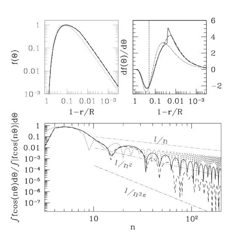
In Fig. 1, we present the numerically obtained damping rates for power-law models with $\beta$ ranging from $1.0$ to $3.0$. Some of these models have double power-law density profiles but only the envelope $\beta$ value affects the scaling for the damping rates. These numerical results confirm our above analytical scalings.

We have also computed damping rates using realistic Jupiter models published by Guillot et al. (2004). These models are discussed in Appendix A and have $\beta=1.8$ in the outer envelope. The numerical results are shown in Fig. 2. They follow the scalings derived above and can be summarized as,

$$\gamma = 6\times 10^{-13}\left({\lambda\over{7.59}}\right)^{7.1}\hskip 28.90755pt{\mbox{for $\lambda<50$}},$$ (21)

$$= 3\times 10^{-9}\left({\lambda\over{7.59}}\right)^{3}\hskip 32.52127pt{\mbox{for $\lambda>50$}},$$

where we have scaled $\lambda$ by $7.59$, the value of $\lambda$ for a low order inertial-mode ($n_{1}=n_{2}=1$). Even this low order inertial-mode is rather more strongly damped than the equilibrium tide. Mode with $\lambda\sim 50$ have $z_{1}\sim z_{\rm crit}\sim 10^{-2.8}R$. Moreover, damping rates depend only on $\lambda$ but not on $(n_{1},n_{2})$ values.

3. Tidal Q for Jupiter

3.1. $Q$ value by Equilibrium Tide

For the equilibrium tide, equation (1) (Goldreich & Soter, 1966) yields $Q_{\rm equi}=\omega/\gamma_{\rm equi}$, where $\omega$ is the tidal frequency in the rotating frame ($\omega=2\omega^{\prime}=2(\Omega-\omega_{\rm Io})=1.532\Omega$), and $\gamma_{\rm equi}$ is the turbulent damping rate for the equilibrium tide as calculated in §2.3.1. Substituting with the value $\gamma_{\rm equi}\sim 4\times 10^{-16}\,\rm s^{-1}$, we obtain $Q_{\rm equi}\sim 10^{12}$, while Goldreich & Nicholson (1977) presented an estimate of $Q_{\rm equi}\sim 5\times 10^{13}$. The discrepancy is partially due to the fact that they have adopted an effective $<\nu>\sim 10^{3}$ while our effective $<\nu>\sim 10^{4}$ (§2.3.1) – the actual viscosity is of course uncertain, easily by a factor of $10$. Moreover, their estimate is more order-of-magnitude in nature. In any case, dissipation of the equilibrium tide, as has been argued long and hard, can not be responsible for the outward migration of Io and other satellites.

3.2. $Q$ value by Inertial-Modes

How much stronger dissipation can inertial-modes bring about? Compared to the equilibrium tide, inertial-modes have the advantage that they can be resonantly driven by the tidal forcing as they are dense in the frequency range of interest (§2.1), and they are damped much more strongly than the equilibrium tide (§2.3.2). The disadvantage, however, lies in the generally weak coupling between an inertial-mode and the tidal potential. Can the first two advantages overcome the last disadvantage? Here, we combine results from previous sections to calculate the tidal $Q$ caused by inertial-modes.

3.2.1 $Q$ value by Individual Modes

We start by calculating the amount of tidal energy dissipated via one inertial-mode. The following forced-damped oscillator equation describes the interaction between an inertial eigen-mode and the tidal forcing,

$$\rho\ddot{\mbox{\boldmath$\xi$}}+\rho\gamma\dot{\mbox{\boldmath$\xi$}}+\rho\omega_{0}^{2}\mbox{\boldmath$\xi$}=-\rho\nabla\delta\Phi_{\rm tide}\exp^{i\omega t},$$ (22)

where $\xi$ is the displacement, and the three terms on the left-hand-side represent, respectively, the inertia, the viscous damping, and the restoring force. The free mode will have an eigenfrequency of $\omega_{0}$. The right-hand-side is the tidal forcing with frequency $\omega$ which we take to be $\omega\approx\omega_{0}$. Adopting the substitution $\mbox{\boldmath$\xi$}=\alpha\tilde{\mbox{\boldmath$\xi$}}$, $\rho^{\prime}=\alpha{\tilde{\rho}^{\prime}}$ with the tilded quantities normalized as $\omega^{2}/2\,\int d^{3}r\rho\tilde{\mbox{\boldmath$\xi$}}\cdot\tilde{\mbox{\boldmath$\xi$}}=1$, multiply both sides by ${\tilde{\mbox{\boldmath$\xi$}}}$ and integrating over the planet, we obtain the amplitude $\alpha$

$$\alpha={{\cal C}\over 2}{{e^{i\omega t}}\over{\left({{\omega_{0}^{2}}\over{\omega^{2}}}-1\right)+{{2i\gamma}\over{\omega}}}}={{\cal C}\over 2}{{\omega e^{i\omega t+i\epsilon}}\over{\sqrt{4(\delta\omega)^{2}+\gamma^{2}}}}$$ (23)

where the tidal coupling ${\cal C}=\int\,d^{3}r\,{\tilde{\rho}^{\prime}}\delta\Phi_{\rm tide}$, the frequency detuning $\delta\omega=\omega-\omega_{0}\approx(\omega^{2}-\omega_{0}^{2})/2\omega$, and the angle $\epsilon=\tan^{-1}(\gamma/2\delta\omega)$ (we assign $\gamma>0$ for damping). For the equilibrium tide ($\delta\omega=\omega$), this angle represents the lag-angle between the tidal bulge and the tide-raising body, $2\epsilon\approx 2\tan\epsilon=\gamma_{\rm equi}/\omega=1/Q_{\rm equi}$ (eq. [1] & §3.1).

Energy in the inertial-mode is simply $\alpha^{2}$, and the energy dissipated via this mode over one period can be found by

$$\Delta E = \oint\,dt\,{{dE}\over{dt}}=\oint\,dt\,\int\,d^{3}r\,{\rm Re}[\dot{\mbox{\boldmath$\xi$}}]{\rm Re}[\rho\nabla\delta\Phi_{\rm tide}e^{i\omega t}]$$ (24)

$$= |\alpha|{\cal C}\oint\,dt\,\omega\sin(\omega t+\delta)\cos(\omega t)$$

$$= |\alpha|{\cal C}\pi\sin\delta={{\omega{\cal C}^{2}\pi\gamma}\over{2(4\delta\omega^{2}+\gamma^{2})}}.$$

The tidal $Q$ is related to the above quantity by eq. (1)

$$Q={{2\pi E_{0}}\over{\Delta E}}={{4E_{0}\gamma}\over{\omega{\cal C}^{2}}}\,\left({{4\delta\omega^{2}+\gamma^{2}}\over{\gamma^{2}}}\right),$$ (25)

where again $E_{0}$ is the energy in the equilibrium tide, and the factor in the parenthesis describes the effect of being off-resonance. This expression can also be derived more simply taking $\Delta E=2\pi/\omega\,\gamma E=2\pi/\omega\,\gamma\alpha^{2}$.

We call a mode “in resonance” with the tide whenever $2|\delta\omega|\leq\gamma$. The $Q$ factor associated with a resonant mode, $Q_{\rm res}$, is proportional to the dissipation rate and inversely proportional to the normalized tidal coupling,

$$Q_{\rm res}={{4E_{0}\gamma}\over{{\cal C}^{2}\omega}}={{128\pi}\over{15}}{{\gamma}\over\omega}\,{{\left(\int{{\rho^{2}r^{6}}\over{\Gamma_{1}p}}dr\right)\,\times\left({{\omega^{2}}\over 2}\int\,\rho\mbox{\boldmath$\xi$}\cdot\mbox{\boldmath$\xi$}d^{3}r\right)}\over{\left[\int{{\omega^{2}\rho^{2}}\over{\Gamma_{1}p}}\psi\varpi^{2}\,\cos(2\phi)\,d^{3}r\right]^{2}}},$$ (26)

where equation (9) is used. Notice here that all dependences on Io’s mass and semi-major axis drop out, leaving only the dependences on the tidal frequency and Jupiter’s internal structure.

How does $Q_{\rm res}$ behave for different inertial-modes? Based on our previous discussions, we introduce the following scalings with $\lambda_{0}$ being the wavenumber of reference,

$$\gamma = \gamma_{0}\left({{\lambda}\over{\lambda_{0}}}\right)^{n_{\gamma}},$$

$${\cal C}_{n} \approx n^{-n_{c}}\approx\left({\lambda\over\lambda_{0}}\right)^{-1.25n_{c}}.$$ (27)

Here, ${\cal C}_{n}$ is the severity of cancellation in the tidal coupling, expressed by equation (10). The factor $1.25$ in the second scaling is needed to accurately relate $n=n_{1}+n_{2}$ to $\lambda$ in the range of interest. The normalized tidal coupling ${\cal C}$ can be related to ${\cal C}_{n}$ as

$${\cal C} = {\cal C}_{n}\,{{\int\delta\Phi_{\rm tide}{{\omega^{2}\rho^{2}}\over{\Gamma_{1}p}}|\psi|d^{3}r}\over{\left({{\omega^{2}}\over 2}\int\rho\mbox{\boldmath$\xi$}\cdot\mbox{\boldmath$\xi$}d^{3}r\right)^{1/2}}}$$ (28)

$$\propto{\cal C}_{n}\,{{(\sqrt{\rho}|\psi|)_{z_{1}}}\over{{(\sqrt{\rho}|\psi|)_{z_{1}}}(n_{1}n_{2})^{1/2}}}$$

$$\propto{{{\cal C}_{n}}\over n}\propto{{{\cal C}_{n}}\over\lambda}.$$

Here, we have used the information that the envelope of $\psi$ scales as $1/\sqrt{\rho}$ in the WKB region, and that every nodal patch in the WKB region contributes comparable amount of kinetic energy to the total budget. Again $z_{1}$ stands for the upper turning point at latitude $\theta=\cos^{-1}\mu$.

These scalings combine to yield the following expression for $Q_{\rm res}$:

$$Q_{\rm res}=Q_{0}\gamma_{0}\left({{\lambda}\over{\lambda_{0}}}\right)^{n_{Q}}=Q_{0}\gamma_{0}\left({{\lambda}\over{\lambda_{0}}}\right)^{n_{\gamma}+2+2.5n_{c}},$$ (29)

where $Q_{0}$ is a constant that depends on Jupiter’s internal structure.

We obtain numerical results using two realistic Jupiter models published by Guillot et al. (2004): models B and D. They are discussed in detail in Appendix A. Of particular relevance is that, while hydrogen metallic phase transition is treated as a smooth transition in model B (interpolated equation of state), model D has a first-order phase transition and the associated density jump occurring around $r/R\approx 0.8$. As a result, ${\cal C}_{n}\sim 1/n^{3}$ ($n_{c}=3$) in model B, while ${\cal C}_{n}\sim 1/2n^{2}$ ($n_{c}=2$) in model D. These scalings are derived analytically in Appendix D, and tested using a toy-model integration. In Fig. 2, we further demonstrate that these scalings indeed apply to inertial-modes, albeit with quite a bit of fluctuations.

From equation (21), we obtain $n_{\gamma}=7.1$ for low-order modes ($\lambda<50$). So $n_{Q}$ is expected to be $16.6$ for model B and $14.1$ for model D. We present numerically calculated $Q_{\rm res}$ in Fig. 2 and they confirm these scalings. Moreover, $Q_{\rm res}$ ranges from $10^{-4}$ for the lowest order inertial-modes to $10^{10}$ for model B (and $10^{8}$ for model D) when $\lambda\sim 50$.

3.2.2 Overall $Q$ Value

If we consider multiple inertial-modes each causing $Q_{i}$, the total effect is

$$Q={1\over{\sum_{i}1/Q_{i}}}.$$ (30)

So at any given tidal frequency, $Q$ is dominated by the mode that contributes the smallest $Q_{i}$. Which mode is this and what is the resulting $Q$ value? We derive analytical scalings here to answer these questions.

At a given forcing frequency, $Q$ values (eq. [25]) for different modes depend on $\lambda$ non-monotonically. Typically, as $\lambda$ increases, $Q$ first decreases and then rises sharply. This is because low-order modes typically are driven off-resonance ($2|\delta\omega|\geq\gamma$) while one can easily find high order modes to be in resonance with the tide. For low-order modes, as $\lambda$ increases, the chance for a good resonance with the tidal frequency improves. This compensates for the fact that tidal coupling weakens with $\lambda$ and

$$Q\approx Q_{\rm res}{{4\delta\omega^{2}}\over{\gamma^{2}}}\approx{{256\pi^{2}\Omega^{2}Q_{0}}\over{\gamma_{0}\lambda_{0}^{4}}}\left({\lambda\over\lambda_{0}}\right)^{n_{Q}-2n_{\gamma}-4}.$$ (31)

Here $n_{Q}-2n_{\gamma}-4=2.5n_{c}-2-n_{\gamma}<0$. For high-order modes that satisfy $2|\delta\omega|\leq\gamma$, increasingly weaker tidal coupling accounts for the fact that $Q$ rises with $\lambda$ as $Q\approx Q_{\rm res}\propto\lambda^{n_{Q}}$. The lowest $Q$ value is to be found around modes that satisfy $2|\delta\omega|=2|\omega_{0}-\omega|\sim\gamma$. This occurs at

$${\lambda\over\lambda_{0}}\approx\left({{16\pi\Omega}\over{\gamma_{0}\lambda_{0}^{2}}}\right)^{1/(n_{\gamma}+2)}.$$ (32)

For Jupiter models, this yields $\lambda\sim 60$ (also see Fig. 2). These are the modes that are most relevant for tidal dissipation. They give rise to a minimum $Q$ value

$$Q\approx Q_{0}\gamma_{0}\left({{16\pi\Omega}\over{\gamma_{0}\lambda_{0}^{2}}}\right)^{n_{Q}/(n_{\gamma}+2)}.$$ (33)

This roughly corresponds to $Q\sim 10^{10}$ for model B, and $Q\sim 10^{8}$ for model D (see more detailed calculation below).

In the following, we confirm and refine the above analytical results by a numerical model. While we have a reasonably good handle on mode damping and tidal coupling, we do not have a perfect Jupiter model nor exact inertial-mode solutions to produce exact mode frequencies. So we could not reproduce exactly the tidal response of Jupiter as a function of Io’s orbital period. Fortunately, this problem can be circumvented. In the following exercise, we produce an artificial spectrum of inertial-modes, with frequencies that satisfy the WKB dispersion relation $\mu=sin(n_{2}\pi/\lambda)$ with $\lambda\approx 2(n_{1}+n_{2})$ (Paper I). To this frequency we add a small random component of order $\delta\mu=\mu/(10n_{1})$, which is of order $1/10$ the frequency spacing between neighboring modes of the same $n_{2}$ value. This random component is to encapsulate our above ignorance but neither its size nor its sign qualitatively affect our conclusion. In this treatment, although we will not be able to obtain the exact tidal response of the planet at each forcing frequency, we can get a reasonable statistical impression. In fact, this is the only logical approach warranted by our current knowledge of the interior of Jupiter.

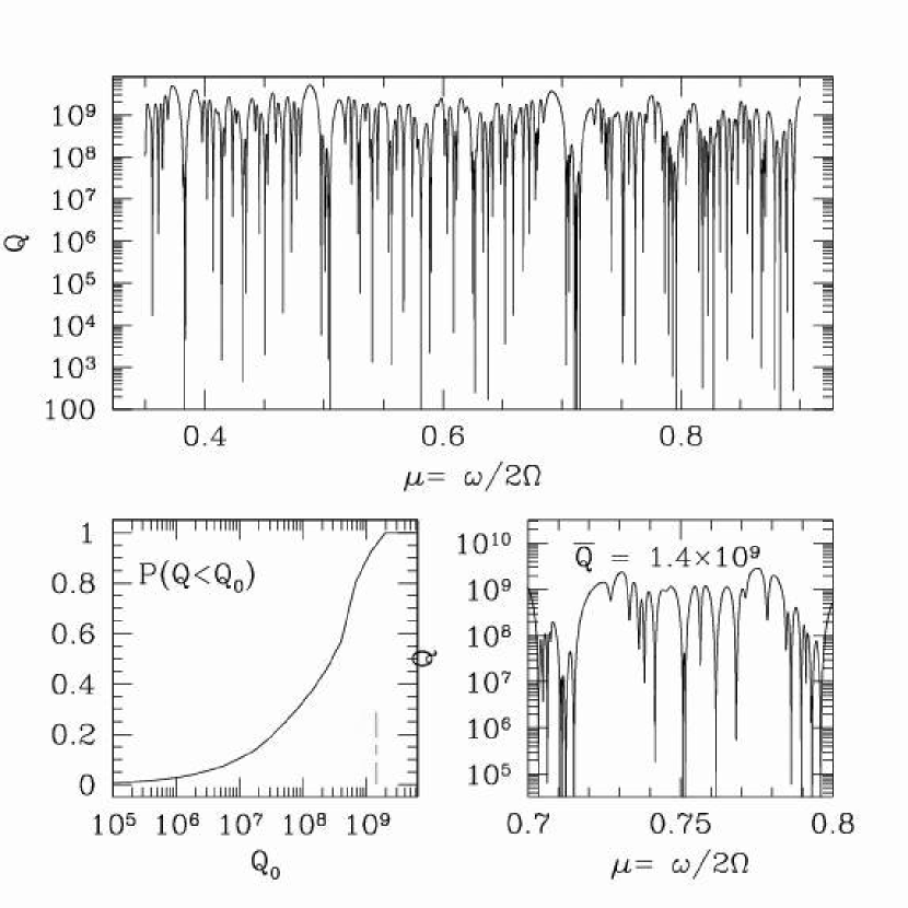
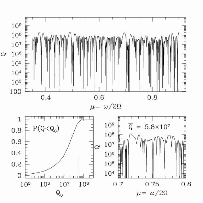
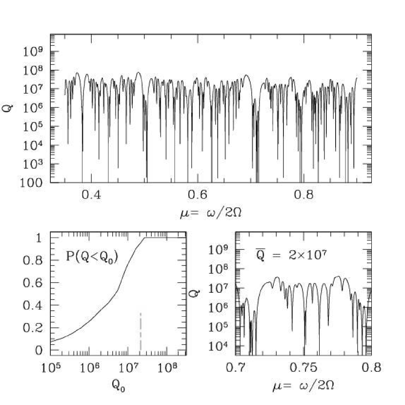
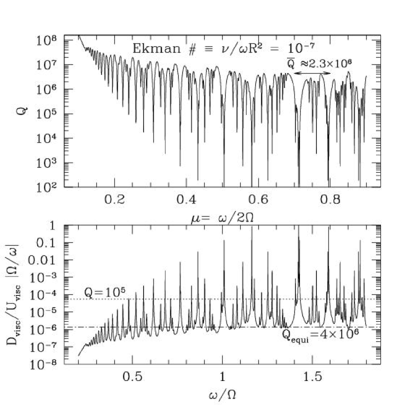
For each inertial-mode, we assign a damping as in equation (21), and a $Q_{\rm res}$ as in equation (29) (different for models B & D), and calculate, as a function of tidal frequency, the $Q$ value for individual modes as well as the overall $Q$ value. The results are presented in Figs. 3 & 4 for the two models. One observes that the $Q$ value fluctuates wildly as a function of the forcing frequency. While there is a ceiling to the overall $Q$ value, there may be occasions when resonance with very low-order modes occurs, leading to deep valleys with $Q$ reaching values as small as $10$. The ceiling, on the other hand, is determined by $\lambda\sim 60$ modes which are always in resonance at any forcing frequency. Due to their high $Q_{\rm res}$ values, modes of orders higher than these are not important.

The results should be interpreted statistically. One can infer from them two pieces of information about Jupiter’s $Q$ value. The first is the average $Q$ value across a certain frequency range, and the second the probability of $Q$ value falling below $10^{6}$ in this frequency range. Here, the value $Q=10^{6}$ is taken to be the rough upper limit for the empirically inferred $Q$ value.

The definition for the word ’average’ deserves some deliberation. We follow Goodman & Oh (1997) and Terquem et al. (1998) in adopting the following average,

$${\bar{Q}}\equiv{{\int_{\mu_{1}}^{\mu_{2}}Q(\mu)Q(\mu)d\mu}\over{\int_{\mu_{1}}^{\mu_{2}}Q(\mu)d\mu}}.$$ (34)

This is equivalent to a time-weighted average since the time a system spends in a certain state is inversely proportional to the torque at that state. Over the evolutionary timescale, the system quickly moves through the deep valleys (large torque) and lingers around in the large $Q$ region. This is also where we most expect to find Jupiter today.

We find that for $\mu\in[0.7,0.8]$, ${\bar{Q}}\approx 1.4\times 10^{9}$ for model B and ${\bar{Q}}\approx 5.8\times 10^{7}$ for model D, roughly consistent with our analytical estimates. Recall that $Q_{\rm equi}\approx 10^{12}$. Moreover, at any forcing frequency, the probability that Jupiter has $Q<10^{6}$ is $3\%$ in model B and $\sim 10\%$ in model D.

4. Discussion

Throughout our calculation, we have assumed that Jupiter is uniformly rotating, neutrally buoyant and core-less. We have also assumed that its internal convection provides a turbulent viscosity which is quantified by the mixing length theory and which is reduced with an index $s=2$ when the convection turn-over time is long compared to the tidal period. We obtained inertial-mode eigenfunctions for realistic Jupiter models using a combination of WKB approximation and exact surface solution (Paper I).

In this section, we discuss the validity of our various assumptions, factors that might influence our results, as well as implications of our results.

4.1. Tidal Overlap

Firstly, a precaution about tidal overlap. We find that this is the trickiest part of our work because inertial-modes propagate essentially over the whole planet, with a small evanescent region very close to the surface. Regions of positive and negative tidal coupling lay side by side, leading to strong cancellation and extreme sensitivity to numerical accuracy. In fact, for a sphere with a density profile that follows a single power-law, the net tidal coupling decreases with increasing mode order so strongly (Appendix C) that numerical precision is soon strained even for fairly low-order modes. Inertial-modes are not important for tidal dissipation in these models.

In a realistic Jupiter model, the cancellation is less extreme due to the following two features: the molecular to metallic hydrogen transition at $r/R\sim 0.8$ (either a discreet phase transition or a continuous change) and the polytropic index change at $r/R\sim 0.98$ where hydrogen molecules change from ideal gas to strongly interacting Coulomb gas (discussed in Appendix A.1). These two features act as some sort of ’internal reflection’ for the inertial-modes – their WKB envelopes inside and outside of these features differ. This weakens the above-mentioned near-perfect cancellation in the overlap contribution from different regions and leads to larger tidal coupling. This is confirmed by integration using both a toy-model (Appendix D) and actual inertial-mode eigenfunctions. In this case, tidal dissipation via inertial-modes outweighs that due to the equilibrium tide.

The inertial-mode eigenfunctions for realistic Jupiter models are constructed as follows (see also Paper I). We first obtain eigenfunctions for a single power-law model with the power-law index ($\beta$) determined by that in the outer envelope of the Jupiter model. This can be done exactly as long as we ignore the Eulerian density perturbation in the equation of motion. We multiply the resulting wave-function by a factor $\sqrt{\rho_{\rm surf}/\rho}$ where $\rho_{\rm surf}$ is the density for the above single power-law and $\rho$ is the actual density. We showed in Paper I that in the WKB region, this construction approximates the actual eigenfunction to order ${\cal O}(1/\lambda^{2})$, and it is exact in the surface evanescent region.

The effects of such a non-exact formulation on mode eigenfrequencies will not significantly alter our results and its effects on the damping rates are negligible. But does it affect our results on tidal coupling, which, as we have shown, depends sensitively even on numerical accuracy? A definitive answer may have to come from high resolution numerical calculations. But our toy-model gives us some confidence that our approach has captured the essence of the problem and that our overlap result is qualitatively correct.

4.2. Turbulent Viscosity

The next issue concerns the turbulent viscosity. We have presented the detailed viscosity profile in Appendix A.2 & Fig. 8.. This is calculated based on the mixing-length theory which is order-of-magnitude in nature (also see eq. [13]). How much does the $Q$ value change when the viscosity is raised (or decreased) by a factor of, say, $100$? The scaling in equation (33) yields $Q\propto\gamma_{0}^{1-n_{Q}/(n_{\gamma}+2)}$, ot $Q\propto\gamma_{0}^{-0.8}$ for model B and $\propto\gamma_{0}^{-0.5}$ for model D. So even a factor of $100$ change in the viscosity causes a change in the $Q$ value that is comparable to our numerical accuracy and is not significant.

Zahn (1977) has advocated a less drastic reduction of the turbulent viscosity when the convective turn-over time is much longer than the tidal period: $s=1$ in equation (13). This produces two differences to our results. First, the equilibrium tidal $Q$ is reduced to $\sim 10^{9}$ as the effective viscosity is increased over the bulk of the planet by a factor of $\sim 10^{3}$. Inertial-modes also in general experience stronger dissipation, with the change more striking for low-order modes. Moreover, modes of lower order can now satisfy the resonance condition ($2|\delta\omega|\approx\gamma$) and they are the dominant modes for tidal dissipation. However, the enhanced $\gamma$ also means every mode now has a larger $Q_{\rm res}$, as a result, the overall $Q$ factor by inertial-modes is hardly modified from that in the $s=2$ case (see Fig. 5).

4.3. Density Discontinuities

As our results in Figs. 3 & 4 show, when there exists a discreet density jump inside Jupiter, the overall $Q$ factor is $\sim 10^{7}$, or $\sim 10^{2}$ times smaller than the case when there is no jump, with $\sim 10\%$ chance that the current $Q$ value falls between $10^{5}$ and $10^{6}$ (the empirically inferred $Q$ range for Jupiter). This dependence on density discontinuity deserves explanation.

It results from a difference in the overlap integral. In the jump case, cancellation in the overlap contribution coming from different parts of the planet is less severe (${\cal C}_{n}\propto 1/n^{2}$), while it is more complete in the no-jump case (${\cal C}_{n}\propto 1/n^{3}$), as is explained using a toy-model in Appendix D. In the no-jump case, the ${\cal C}_{n}\propto 1/n^{3}$ scaling may arise from two causes: a discontinuity in the density gradient due to, for instance, a second-order phase transition, and a sharp transition in the power law index $\beta$ (equivalently, the polytropic index $\Gamma_{1}$) when the equation of state changes. In Jupiter models, the latter occurs at $r/R\sim 0.98$, spanning a range of $\Delta r/R\sim 0.02$, or $\sim 4$ local pressure scale heights (Appendix A.1). The overall $Q$ factor is little affected if either transition region is shifted upward or downward by a few pressure scale heights. However, if the second-order phase transition does not exist, and if the polytropic transition occurring over a range $\Delta r/R\gg 0.02$, we expect ${\cal C}_{n}\propto 1/n^{4.6}$ and the overall $Q$ factor to be much larger.

Does Jupiter harbor a density jump?

One possibility is the so-called metallic hydrogen phase transition. Our knowledge of the equation of state for hydrogen at Mbar level is currently limited. We do not know whether the transition from a molecular fluid to a conductive fluid (metallic hydrogen) is a plasma phase transition (PPT) with a discreet density jump, or a continuous process with only a jump in the density gradient. And in the case of PPT, we do not know whether the actual Jovian adiabat falls below or above the critical temperature for a first-order transition (Stevenson, private communication). Plighted by these uncertainties, planet modelers have typically chosen to insert (or not to insert) by hand a small density jump at the suspected PPT location, and then interpolated between very low and very high pressures (where we know the equation of state well), under certain assumptions, to obtain the pressure-density curves around this point. We build our analysis on two examples of such models (model B with a smooth transition and model D with a jump). Interestingly, Guillot et al. (2004) showed that among models that match all observational constraints on Jupiter, the ones with PPT equation of state have larger core mass and lower total mass of heavy elements, while the ones with smooth interpolated equation of state tend to the opposite.

Another possibility may follow from helium/hydrogen phase separation. Whenever the Jovian adiabat falls below the critical temperature curve for helium immiscibility, helium separates from hydrogen and forms helium-rich droplets that fall toward the center (Salpeter, 1973). Due to its cooler interior, this process has proceeded further in Saturn than in Jupiter. But even in Jupiter there may be a density jump, or at worst, a jump in density gradient, associated with this effect.

Close-in hot exo-jupiters presumably have higher overall entropy than Jupiter does, as radiation from their surface is effectively sealed off by the stellar insulation. Their interior temperature is higher at a given pressure. Both PPT and helium rain-out are therefore less likely to occur in these bodies.

In summary, current Jupiter models exhibit features that warrant $Q\sim 10^{9}$. It is plausible to find a non-negligible density jump in the Jovian interior, due either to a first-order PPT or helium/hydrogen separation, in which case we obtain $Q\sim 10^{7}$. This, however, is more difficult to justify in hot exo-jupiters, compromising our initial goal of searching for a universal mechanism.

4.4. Presence of a Solid Core

We have assumed here that convection penetrates into the center of Jupiter. But it is possible that Jupiter does have a solid core. Dermott (1979) pointed out that body tide in the (imperfectly elastic) solid core of Jupiter with a core quality factor $\sim 30$ can account for the observed tidal dissipation. However, this requires a core size which is at the upper-end of current determinations ($r_{\rm core}/R\sim 0.15$) as well as a core quality factor which is currently unknown. Moreover, the efficiency of such a mechanism depends sensitively on the core size and it may be unreasonable to expect that exo-jupiters all have core sizes within a narrow range. So we restrict ourselves to consider the effect of a core on the tidal $Q$ factor due to inertial-modes.

Inertial-modes are excluded from the solid-core. For an estimate, we retain the inertial-mode eigenfunctions calculated for the core-less case, but suppress from the core region contribution to mode energy, mode damping, and tidal overlap integral. We find no substantial difference between this and the core-less case (one can also compare results from model B which is core-less and model D which has a $10M_{\oplus}$ core). Contribution from the core region to the overlap integral, for instance, is insignificant as the radial integrand drops as $\propto r^{6}$ (eq. [C3]): radial dependence of the tidal potential goes as $r^{2}$, and inertial-modes are more anelastic (small $\rho^{\prime}$) in the high density region.

A more subtle influence of the core, however, may be present. While we have been able to separate spatial variables and calculate inertial-mode eigenfunctions in the ellipsoidal coordinates for core-less models, the presence of a spherical core destroys this convenience. The inner boundary conditions can no longer be defined along constant ellipsoidal coordinate curves and we have to return to the original partial differential equations. This is analogous to the situation where the Coriolis force breaks the symmetry of a spherical star, with the result that the angular dependence of an eigen-mode in a rotating star can no longer be described by a single spherical harmonic but only by a mixture of them. So it is perceivable that, if we adopt core-less inertial-mode eigenfunctions as a complete basis, inertial-mode eigenfunction in the presence of a spherical core may be a mixture of these functions. This gives us a hint on how to proceed when there is a core. It is possible to obtain the mixing ratio and use these to calculate new damping rates, mode energy and tidal coupling. We conjecture that the mixture becomes purer (more dominated by one component) as the core size approaches zero. In particular, we expect the mixing not to be important when the core size is much smaller than a wavelength of the inertial-mode ($r_{\rm core}/R\ll 1/\lambda$). We plan to extend our calculation to the solid core case in the future.

The above conjecture seems to be supported by numerical calculations by Ogilvie (2005). He recovers low-order inertial-modes when he decreases the core size. When the core size is significant, however, OL’s study discovered something else. Instead of global inertial-modes, they found that fluid response to the tidal forcing is concentrated into characteristic rays which become singularly narrow as viscosity goes to zero. This appears a rather different picture from ours and the physical origin of these singular rays deserves understanding.

4.5. Radiative Atmosphere

We have also assumed that the convection zone extends all the way to zero density. This may be unrealistic for Jupiter, and worse still for exo-jupiters. In the Jupiter models we adopted, convection gives way to radiation just above the photosphere ($p=1bar$). The reality is more complicated (also see discussions in Paper I). Temperature in the Jovian atmosphere is such that as a fluid parcel travels upward, its water content condenses and releases latent heat. The resulting adiabatic gradient (the ’wet adiabat’) depends on the water content and is shallower than the one that does not include water condensation (the ’dry adiabat’). So for a given temperature profile, a particularly dry parcel can be convectively stable. This is consistent with the Galileo probe data which indicates stable stratification down to $\sim 20bar$ after entering a dry spot on Jupiter(Allison & Atkinson, 2001). Available Jupiter models are at best 1-D representation of the 3-D structure, and our results depend critically on the temperature structure and turbulent viscosity in the upper atmosphere of Jupiter.

What is the effect of a thin radiative atmosphere on inertial-modes? Inertial-modes may not be perfectly reflected near the surface and some of its wave-flux can be smuggled out of the convective region in the form of gravity-waves. The radiative zone has a peak Brunt-Väisälä   buoyancy frequency

$$N\sim{g\over{c_{s}}}\sim{{2700}\over{9.3\times 10^{4}}}\sim 0.029\,\,\rm s^{-1},$$ (35)

which is much higher than the inertial-mode frequencies we are interested in ($\omega\sim 3.5\times 10^{-4}\,\rm s^{-1}$). So the relevant gravity-wave is high in radial order and is strongly modified by rotation, satisfying $N\gg\omega\sim\Omega$. Such waves can be calculated (semi)-analytically under the ’traditional approximation’ and are called the ’Hough modes’. The smuggled wave-flux is subsequently lost in the higher atmosphere where the gravity-wave breaks. This brings about enhanced damping to the inertial-mode. Recall that the overall $Q$ factor scales roughly as inverse square root of the damping rate. So unless the resultant damping rate is orders of magnitude above the rate of turbulent damping, the overall $Q$ factor is little affected.

There are other ways in which a radiative envelope may affect inertial-modes. The upper-turning point ($z/R\sim 1/\lambda^{2}$ when $\theta\sim\cos^{-1}\mu$ and $z/R\sim 1/\lambda$ otherwise) of a sufficiently high order inertial-mode may fall near or above the convective-radiative interface. When this occurs, the structure of the inertial-mode is significantly modified. The radiative region imposes a different surface boundary condition on the inertial-mode than the one we assume here (vanishing Lagrangian pressure perturbation). This different boundary condition, as is illustrated by the toy model in Appendix D, may give rise to much different (likely larger) tidal overlap and therefore a different $Q$ (likely smaller) factor (see also §4.8).

Extra-solar hot jupiters are strongly irradiated by their host stars. Their atmosphere is more isothermal leading to a substantially thicker radiative envelope (down to $\sim 30\,\rm km$ below photosphere) than that in Jupiter. This envelope may sustain rotationally-modified gravity-waves (’Hough Modes’) which may be resonantly (if these waves are trapped) excited by the tidal potential. It is possible that this explains the tidal dissipation in these hot jupiters (Lubow et al., 1997). However, inertial-modes should still exist and will couple to the tidal potential even in these planets. The fact that the $Q$-values appear to be similar between the exo-jupiters and our Jupiter leads us to suspect that inertial-modes will remain relevant. It is foreseeable, for instance, that these planets harbor a new branch of global modes which are inertial-mode like in the interior and gravity-mode like in the exterior.

4.6. Where is the tidal energy dissipated?

In our picture of resonant inertial-mode tide, most of the tidal dissipation occurs very near the surface, where both the kinematic viscosity and the velocity shear are the largest. In a realistic Jupiter model, the effective turbulent viscosity peaks at a depth of $\sim 60\,\rm km$ ($z_{\rm crit}$, Fig. 8 in Appendix A.2), and decays sharply inward. Meanwhile, the displacement caused by inertial-modes rises outward toward the outer turning point. And the velocity shear reaches its maximum inside the ’singularity belt’ (Paper I), which is found to be around $\theta\approx\cos^{-1}\mu$, with an angular extent $\sim R/\lambda$ and a depth $\sim R/\lambda^{2}$. For inertial-modes most relevant for tidal dissipation ($\lambda\sim 60$), this depth roughly coincides with the location of maximum viscosity. We have confirmed numerically that most of the dissipation indeed occur in this shallow belt.

The tidal luminosity in Jupiter is $\sim 7\times 10^{20}(10^{6}/Q)\,\rm erg/\,\rm s$. What is the effect of depositing this much energy in a shallow layer? We compare this against intrinsic Jovian flux of $F\sim 5000\,\rm erg/\,\rm cm^{2}/\,\rm s$. The total intrinsic luminosity passing through the belt is $\sim 2\pi R^{2}/\lambda F\sim 3\times 10^{22}\,\rm erg/\,\rm s$. This is larger than (or at worst comparable to) the tidal luminosity. Another way of phrasing this is to say that the local thermal timescale is shorter than (or at worst comparable to) the ratio between local thermal energy and the tidal flux. So the belt is expected to be able to get rid of the tidal energy without suffering significant modification to its structure.

Angular momentum is also deposited locally. We assume here that the convection zone is able to diffuse the excess angular momentum almost instantaneously toward the rest of the planet. However, if convective transport is highly anisotropic and prohibits diffusion, it is possible that this (negative) angular momentum is shored up near the surface and contributes to surface meteorology of Jupiter.

The transiting planet HD209458b is observed to have a radius of $\sim 1.3R_{J}$ (Brown et al., 2001). Its proximity to its host star and its currently near-circular orbit raise the possibility that its over-size is a result of (past or current) tidal dissipation (Gu et al., 2003). However, if our theory applies also to these hot jupiters, we would expect that the tidal heat is deposited so close to the planet surface that it can not be responsible for inflating the planet. Moreover, given the short local thermal timescale, any change to the planet structure should disappear once tidal dissipation ceases.

4.7. Tidal Amplitude and Nonlinearity

If inertial-modes are resonantly excited to large amplitudes, they can transfer energy to other inertial-modes in the planet and be dissipated by nonlinear mode coupling. To see whether this is important, we consider the amplitude of inertial-modes. This is largest near the surface around the ’singularity belt’. When an inertial-mode is resonantly excited ($|\delta\omega|\leq\gamma$), we obtain a horizontal surface displacement $\xi_{h}\sim 10^{11}(\lambda/7.59)^{-7}\,\rm cm$. While this implies extreme amplitudes for low-order modes, they only come into resonance rarely. For modes of interest ($\lambda\sim 60$), the typical surface displacement amplitude is $\sim 10^{3}\,\rm cm$, so the dimensionless amplitude ($\xi/R_{J}$) is $10^{-7}$. Can such an amplitude incur strong nonlinear damping?

At such small amplitudes, nonlinear effects can be well described by three-mode couplings. The efficiency of this process scales with the amplitudes of the modes concerned. The most important nonlinear coupling is parametric resonance: when the inertial-mode reaches a threshold amplitude, pairs of daughter inertial-modes, at half the frequency and with $m=-1$, can be parametrically excited and can grow to significant amplitudes. Nonlinear mode coupling then drains energy quickly out of the original mode. The threshold dimensionless amplitude is (Landau & Lifshitz, 1969; Wu & Goldreich, 2001)

$$\left.{\xi\over{R_{J}}}\right|_{\rm para}\approx{1\over\kappa}\left[\left({{\gamma_{2}}\over{\omega}}\right)^{2}+\left({{\delta\omega}\over{\omega}}\right)^{2}\right]^{1/2},$$ (36)

where $\kappa$ is the coupling coefficient between the parent and the daughter pair, $\gamma_{2}$ the damping rate for the daughter modes, and $\delta\omega$ the frequency detuning for this resonance. Arras et al. (2003) has studied the coupling coefficient for inertial-modes in a uniform density sphere and found $\kappa\leq n_{1}/\mu^{2}$: the maximum coupling coefficient obtains for daughter pairs that are spatially similar and maximally overlap. We adopt their result here. We further take $\delta\omega=0$ and $\gamma_{2}=\gamma_{1}\sim 10^{-7}$ to obtain the lowest possible threshold amplitude. For inertial-modes of interest, ${\xi/R_{J}}|_{\rm para}\sim 10^{-3}$. So parametric damping of the tidally forced inertial-modes is un-important.

Another three-mode coupling of consequence is between the inertial-mode, itself and a mode at twice the frequency (up-conversion). However, in the case of Jupiter, twice the tidal frequency falls outside the inertial-mode range.

Unconsidered here is another form of parametric resonance: simultaneous excitation of two inertial-modes by the tidal potential, with frequencies of the two modes summing up to the tidal frequency. We find this to be also negligible for Jupiter-Io system, but likely important for exo-jupiters.

4.8. Comparison with Ogilvie & Lin (2004)

The most relevant work to compare our results against is that of OL, which is an independent study that appeared while we were revising our paper. In their work, the same physical picture as that discussed here was considered, namely, tidal dissipation in a rotating planet. They employed a spectral method to solve the 2-D partial differential equations which describe fluid motion forced by the tidal potential inside a viscous, anelastic, neutrally buoyant, polytropic fluid. This procedure directly yields the value of the tidal torque on the planet, without the need of a normal mode analysis. The numerical approach allows them to include the effect of a solid core, as well as that of a radiative envelope. Overall, they concluded that inertial-waves can provide an efficient mechanism for tidal dissipation, and that the tidal $Q$ factor is an erratic function of the forcing frequency. We concur with these major conclusions.

However, many technical differences exist between the two works. To better understand both works, it is illuminating to discuss some of these differences here.

Firstly, as is mentioned in §4.4, while we obtain global inertial-modes which have well defined WKB properties and discreet frequencies, OL demonstrated that the tidally-forced response of a planet is concentrated into characteristic rays which are singular lines in the limit of zero viscosity. While viscous dissipation in their case occurs in regions harboring these rays, our inertial-modes are predominately dissipated very near the surface (the ’singularity belt’). Moreover, although both our $Q$ values exhibit large fluctuations as a function of tidal frequency, the origin of the two may be different – in our case, a deep valley indicates a good resonance between the tide and a low-order inertial-mode, while the situation is less clear in their case. All these differences may originate from the presence (absence) of a solid core in their (our) study. We are currently investigating the underlying mathematical explanation for these differences. Again, it is interesting to note that as the core size approaches zero, inertial-modes seem to reappear (Ogilvie, 2004, private communication).

Secondly, OL’s results are based on a $n=1$ polytrope, for which we find that tidal coupling is vanishingly small (see Appendix C), and that inertial-modes are not important for tidal dissipation. It is currently unclear whether this difference arises from the presence of a core or from the presence of a radiative envelope in their study. Despite a steep suppression of the tidal overlap integrand near the center (integrand $\propto r^{6}$), the presence of a solid core may affect tidal overlap in a more substantial manner by reflecting inertial-waves and changing their mode structure (§4.4). Meanwhile, a surface boundary condition specified at a finite density (instead of at $\rho=0$) may cause extra tidal coupling (§4.5), as is shown by the analysis in Appendix C. This issue is more relevant for extra-solar hot jupiters which have deeper radiative envelopes.

Thirdly, OL assumed a constant Ekman number throughout the entire planet. Since

$$Ek\equiv{{\gamma}\over{\omega}}={{\nu}\over{\omega R^{2}}},$$ (37)

this implies a viscosity $\nu=\omega R^{2}Ek\sim 2\times 10^{16}Ek$ that is constant throughout the planet. We have argued that the effective viscosity value for the equilibrium tide should be of order $\sim 10^{4}\,\rm cm^{2}/\,\rm s$ (§2.3.1), or an effective $Ek\sim 10^{-13}$. However, such a weak viscosity is much smaller than is currently reachable by a numerical method in a reasonable amount of time. Instead, OL have opted for an alternative treatment in which they steadily decreased the Ekman number from $Ek=10^{-4}$ to $10^{-7}$ and argued (based both on numerical evidence and on an analytical toy-model) that the final $Q$ value is independent of the Ekman number. This contrasts with our results that $Q$ roughly scales as $\gamma_{0}^{-1/2}$ (§4.2), obtained for realistic viscosity profiles, where $\gamma_{0}$ is the damping rate for a mode of wavenumber $\lambda_{0}$.

To make the comparison more appropriate, we adopt a constant viscosity inside the planet and find that mode damping rates $\gamma=5\times 10^{-9}(Ek/10^{-7})\,(\lambda/7.59)^{3.0}\,\rm s^{-1}$ in the Jupiter model D, while individual mode $Q_{\rm res}$ value also scales linearly with the Ekman number (eq. [26]). Applying scalings derived in §3.2.1, we find an overall $Q\sim 2.3\times 10^{6}(Ek/10^{-7})^{-1}$. This value is consistent with that obtained by OL for $Ek\sim 10^{-7}$. Meanwhile, the equilibrium tide gives rise to $Q_{\rm equi}\sim 4\times 10^{6}(Ek/10^{-7})^{-1}$. So in models of a constant Ekman number, inertial-modes contribute comparably to tidal dissipation as does the equilibrium tide, but no better. These results are presented in Fig.6.

5. Summary

In a series of two papers (Paper I & this), we have examined the physical picture of tidal dissipation via resonant inertial-modes. This applies to a neutrally-buoyant rotating object in which the tidal frequency in the rotating frame is less than twice the rotation frequency.

In Paper I, we first demonstrate that under some circumstances (power-law density profiles of the form $\rho\propto(1-r^{2})^{\beta}$), the partial differential equations governing inertial-modes can be separated into two ordinary differential equations with semi-analytical eigenfunctions. We also show that this method can be extended to apply to more general density profiles, with the price that the solution is exact in the surface region but only approximate in the WKB regime. Nevertheless, this approximate solution allows us to draw many physical conclusions concerning inertial-modes, including their spatial characteristics, their dispersion relation, their interaction with the tidal potential and with turbulent convection. This semi-analytical technique gives us an edge over current computational capabilities, though full confirmation of our conclusions may require careful and high-resolution numerical computation. It is clear from our study that any numerical approach would need to be able to resolve the so-called “singularity belt” near the surface where inertial-modes vary sharply, and that numerical results need to be taken cautiously when evaluating the tidal overlap.

In this paper, we discuss the role in tidal dissipation played by inertial-modes. This depends on the following three parameters: how well coupled an inertial-mode is to the tidal potential, how strongly dissipated an inertial-mode is by turbulent viscosity, and how densely distributed in frequency are the inertial-modes. We have obtained all three parameters using both toy models and realistic Jupiter models. Low-order inertial-modes, if in resonance ($\delta\omega<\gamma$, where $\delta\omega$ is the frequency detuning between the tidal frequency and the mode frequency, $\gamma$ is the mode damping rate), can dissipate tidal energy with $Q$ as small as $Q\sim 10$. However, such a resonance is not guaranteed at all tidal frequencies, and the system sweeps through a fortuitously good resonance with speed. Inertial-modes most relevant for tidal dissipation are those satisfying $\delta\omega\sim\gamma$, where $\delta\omega$ decreases with mode wave-number as $\delta\omega\propto\lambda^{2}$, and $\gamma$ rises steeply with mode wave-number. These are inertial-modes with wave-numbers $\lambda\sim 60$ (or total number of nodes $n=n_{1}+n_{2}\sim 30$). At any tidal frequency, one can always find resonance with one such mode. They provide the continuum to the $Q$ value, whereas previously mentioned good resonances appear as dense valleys superposed on this continuum (see, e.g., Fig. 4).

The continuum $Q$ value depends sensitively on the presence of density discontinuities inside Jupiter, as the latter influences strongly the magnitude of coupling between the tidal potential and inertial-modes. Current Jupiter models show a sharp change in the adiabatic index near the surface (hydrogen ideal-gas to Coulomb gas transition), this warrants a $Q$ value of $\sim 10^{9}$. The presence of a discontinuity in density gradient due to a phase transition (metallic hydrogen phase transition and/or helium/hydrogen separation) has the same effect. On the other hand, if the phase transition is first-order in nature and incurs a density jump, $Q\sim 10^{7}$. Our results are uncertain up to perhaps, one order of magnitude. But it is already clear that inertial-modes cause much stronger dissipation than the equilibrium tide, which yields $Q_{\rm equi}\approx 10^{12}$. In the case of $Q\sim 10^{7}$, there is a $\sim 10\%$ chance that the current $Q$ value falls between $10^{5}$ and $10^{6}$ (the empirically inferred $Q$ range for Jupiter).

Our model also builds on the assumption that Jupiter is neutrally stratified and turbulent all the way up to the photosphere, as turbulent dissipation for inertial-modes with $\lambda\sim 60$ are calculated to arise mostly near or below the photospheric scale-height. Effects like water condensation may alter the static stability in Jupiter’s atmosphere, making the atmospheric stratification a function of space and time.

We also restrict ourselves to core-less Jupiter models. Our conclusion is little affected when we include an inner core with a size that is compatible with current constraints. However, this is assuming that global inertial-modes still exist in the presence of a solid core. Ogilvie (2005) extended the study in Ogilvie & Lin (2004) and demonstrated that a new kind of tidal response appears when Jupiter has a core: fluid motion is tightly squeezed into ’characteristic rays’ which becomes singular when the viscosity goes to zero. This is a drastically different picture than the global eigenmode picture described here and may lead to different $Q$ factors.

We have adopted the Goldreich & Keeley (1977) prescription ($s=2$) to account for the reduction in turbulent viscosity when the convective turn-over time is long relative to the forcing period. Calculations adopting Zahn’s prescription ($s=1$) produce no difference in the $Q$ value caused by inertial-modes, though we find the equilibrium tide is significantly more strongly damped. Concerning possible effects of nonlinearity: The surface movement of inertial-modes is predominately horizontal. For inertial-modes that are most relevant for tidal dissipation, the surface displacement amplitude $\sim 10^{3}\,\rm cm$, or $\sim 10^{-7}$ of the radius. We estimate that nonlinear effects are negligible.

In our theory, tidal heat is deposited extremely close to the planet surface (inside the ’singularity belt’) and can be lost quickly to the outside. For Jupiter, the tidal luminosity in this region is smaller than (or at worst comparable to) the intrinsic luminosity and so would not much alter the structure. However, there remains the intriguing possibility that the negative angular momentum deposited to the belt may affect surface meteorology (jet streams and anticyclones). Moreover, if this theory also applies to hot exo-jupiters, the tidal luminosity is unlikely to be responsible for inflating planets and solving the size-problem of close-in exo-jupiter HD209458b.

Although our investigation was stimulated by the fact that exo-solar planets exhibit similar $Q$ values as Jupiter does, it may be difficult to draw a close analogy between Jupiter and hot exo-jupiters: the existence of a first-order phase transition is less convincing in the latter due to their hotter interiors; the upper atmosphere of these planets are strongly irradiated by their host stars and are therefore likely to be radiative; they may have rather different core sizes depending on their formation history. Nevertheless, it is our plan to extend the current study to exo-jupiters, as investigations into these bodies may ultimately yield clue for the story of Jupiter. It is also foreseeable that the theory developed here has implications for Saturn, Uranus, solar-type binaries, M-dwarfs and brown-dwarfs.

Figure 1.— Numerically computed turbulent damping rates for inertial-modes in various power-law models, as a function of the mode wavenumber $\lambda$. Here, we have taken the reduction number $s=2$ and included damping rates only for modes with $n_{1}\sim n_{2}$, though other modes satisfy the same scalings observed here. Models a & b are single power-law models, while c & d are double power-law models ($\beta_{1}$ the index in the interior and $\beta_{2}$ that in the envelope) with the transition of $\beta$ occurring around $r/R\sim 0.98$. All models are normalized to have the same central density and their viscosity profiles are described by equations (A2)-(A3). The dotted lines are power-law fits to the numerical results with the numerical scalings summarized in the top-left corner. These are well reproduced by our analytically derived relation $\gamma\propto\lambda^{3.5+2\beta_{2}}$ (eq. [19]). Notice that only the envelope power-law index enters the relation. Damping rates in all models flatten at large $\lambda$, and scale with $\lambda$ roughly as $\lambda^{3}$ (eq. [20]).

Figure 2.— Tidal coupling, viscous damping rate and resonant $Q_{\rm res}$ factor for various inertial-modes calculated using two Jupiter models. Model B (open circles) has no heavy metal core and no first-order metallic hydrogen phase transition, while model D (solid triangles) has a core as well as a density jump at $r/R\sim 0.8$ due to the plasma phase transition. The upper-left panel presents the (normalized) coupling integral ${\cal C}_{n}$ (eq. [10]) as a function of inertial-mode node numbers ($n=n_{1}+n_{2}$). Although the scatter is large, model B results are best fit by ${\cal C}_{n}\sim 1/n^{3}$ (solid line), while model D results follow ${\cal C}_{n}\sim 1/2n^{2}$ (dotted line). The lower-left panel shows the energy damping rate as a function of mode wavenumber $\lambda$ ($\lambda\sim 2n$). Results from both models scale as $\lambda^{7.1}$ for low-order modes and as $\lambda^{3}$ for high-order modes (two solid lines), consistent with analytical expectations (§2.3.2). The dotted line in the same panel is the minimum frequency detuning as a function of $\lambda$ (eq. [4]). $Q_{\rm res}$, the $Q$ value contributed by each mode when it is in resonance with the tide (eq. [26]), is plotted on the right-hand panel as a function of $\lambda$. Again, analytical expectations for models B & D are depicted by the solid and dotted lines, respectively. While low-order modes ($\lambda<40$) from the two models largely share similar $Q_{\rm res}$ values, higher order modes follow more closely the analytical scalings. Here, we have included only inertial-modes with $\mu\sim 0.776$ but the results remain similar for other inertial-modes.

Figure 3.— Numerically calculated values of $Q$ for model B. The upper panel shows $Q$ as a function of the tidal frequency in the rotating frame. Deep dips occur whenever the tide is in resonance with a low-order inertial-mode ($\lambda\ll 60$), and the ceiling to the $Q$ value is determined by the group of modes with $\lambda\sim 60$ which satisfy $2|\delta\omega|\sim\gamma$. The tide is always in resonance with one of these modes at any frequency. The lower left panel shows the cumulative probability distribution of the $Q$ value within the frequency range $0.7<\mu<0.8$. At a given frequency there is $\sim 3$ percent chance that we will find $Q<10^{6}$. The probability for this to occur at a given instant in time is smaller. The dashed vertical curve locates the time-weighted average $Q$ value (${\bar{Q}}$, eq. [34]). We find ${\bar{Q}}=1.4\times 10^{9}$ within this frequency range. The lower right panel expands the view of the upper panel over this frequency range. The locations of the fine structure in this plot are not to be taken literally as we have adopted an approximate dispersion relation for the inertial-modes.

Figure 4.— Same as Fig. 3, but for model D in which the tidal coupling decreases as $1/2n^{2}$ as opposed to $1/n^{3}$. This is related to the presence of a first-order phase transition at $r/R\sim 0.8$. While showing overall similar characteristics as those in Fig. 3, ${\bar{Q}}$ has now been reduced to $\sim 5.8\times 10^{7}$ between $\mu=0.7$ and $0.8$, and at any given tidal frequency, there is a $\sim 10\%$ chance that Jupiter exhibits $Q<10^{6}$.

Figure 5.— Same as Fig. 4, but calculated for model D when the index for viscosity reduction is taken to be $s=1$ (Zahn, 1977) instead of $s=2$. Mode damping rates now behave as $\gamma=10^{-10}(\lambda/7.59)^{4.5}\,\rm s^{-1}$. We obtain ${\bar{Q}}\approx 2\times 10^{7}$, with $\sim 30\%$ chance that $Q<10^{6}$ for the current tidal frequency. Moreover, $Q_{\rm equi}\approx 10^{9}$ in this case.

Figure 6.— We repeat our calculation for model D, taking the turbulent viscosity to be a constant throughout the planet with the Ekman number $Ek=\nu/\omega R^{2}=10^{-7}$. Mode damping rates scale much less steeply with inertial-mode wave-numbers, $\gamma=5\times 10^{-9}(\lambda/7.59)^{3.0}\,\rm s^{-1}$. The resulting $Q$ value from inertial-modes is plotted against $\mu$ in the upper panel, with ${\bar{Q}}\approx 2.3\times 10^{6}$ over the range $\mu\in[0.7,0.8]$. A similar calculation for model B yields ${\bar{Q}}\approx 3.5\times 10^{6}$. We find that the ${\bar{Q}}$ value is inversely proportional to the Ekman number. The lower panel translates the $Q$ result into a quantity used in Fig. A2 of OL (the dimensionless viscous dissipation rate, $\propto 1/Q$), plotted here as a function of $2\mu=\omega/\Omega$. The two overlaid lines with $Q=10^{5}$ (dotted) and $Q=4\times 10^{6}$ (dot-dashed), respectively represent the empirically inferred $Q$ value for Jupiter and the $Q$ value associated with the equilibrium tide in this model. These results resemble those presented in Fig. A2 of OL for the same Ekman number.

Appendix A Relevant Properties in a Jupiter Model

Here, we study properties of Jupiter that are relevant for the tidal process. This is based on publicly available models of Jupiter presented in Guillot et al. (2004). They are produced with the newest equation of state and opacity calculations, including the effect of hydrogen phase transition, and alkali metal opacity. They satisfy gravity measurements (esp. $J_{2}$ & $J_{4}$) to much better than a percent and reproduce other global properties of Jupiter (radius, surface temperature, intrinsic flux).

In this study, we focus on two models, B and D, out of the five sample models presented in Guillot et al. (2004). Model B is produced with an interpolated hydrogen equation of state (meaning no first-order metallic hydrogen phase transition), and has no heavy metal core. Model D, in contrast, contains a first-order phase transition (PPT equation of state) and has a core with mass $10M_{\oplus}$. The photosphere for both these models is located at a radius of $\approx 7\times 10^{9}\,\rm cm$, at a pressure of $\approx 10^{6}\,\rm dyne/\,\rm cm^{2}$, and with a temperature $170\,\rm K$ and a density $1.6\times 10^{-4}\,\rm g/\,\rm cm^{3}$.

The interiors of these models are fully convective (outside the core). Due to the high density in Jupiter (mean density $\sim 1.3\,\rm g/\,\rm cm^{3}$), the convection speed needed to carry the small intrinsic flux ($5.4\times 10^{3}\,\rm erg/\,\rm s/\,\rm cm^{2}$) is highly subsonic, resulting in an almost exactly adiabatic temperature profile (super-adiabatic gradient $\sim 10^{-8}$ or smaller). This justifies our assumption of neutrally buoyant fluid when investigating inertial-modes. Only the thin atmosphere above the photosphere, with a local pressure scale height $\sim 20\,\rm km$, is radiative.

A.1. Density Profile

Two features in the density profile of these models deserve attention.

At radius $r/R\sim 0.8$, pressure $\sim 10^{12}\,\rm dyne/\,\rm cm^{2}$, and density $\sim 1\,\rm g/\,\rm cm^{3}$, hydrogen undergoes a phase transition. Above this layer, hydrogen is mostly neutral and molecular. Below this layer, the mean atomic spacing becomes smaller than a Bohr radius and electrons are pressure ionized. The strong Coulomb interaction and electron degeneracy resemble those in a metal and the transition is referred to as ’liquid metallic hydrogen’ transition (Guillot et al., 2004). The nature of this transition is still poorly understood. Model B assumes this transition is of second-order and entails a discontinuity only in the gradient of density (of order $50\%$), while model D assumes it is a first-order transition with a density jump of order $10\%$. These two different treatments should bracket the actual equation of state of hydrogen.

Another feature sets in nearer the surface, at radius $r/R\sim 0.98$, pressure $\sim 10^{10}\,\rm dyne/\,\rm cm^{2}$ and density $0.1\,\rm g/\,\rm cm^{3}$. Above this region, the gas can be considered as ideal diatomic gas ($H_{2}$). As the temperature is below $2000\,\rm K$, the mean degree of freedom for each molecule is $5$ (three translational plus two rotational). The specific heat per molecule at constant volume and constant pressure are, respectively, $C_{V}=5/2k_{B}$, $C_{p}=7/2k_{B}$, yielding $\Gamma_{1}={\partial\ln P/\partial\ln\rho}|_{s}=C_{p}/C_{V}=1.4$. Below this region, however, $\Gamma_{1}$ rises to $\sim 1.8-2.2$ in the main body of the planet, and approaches $3$ in the very deep interior (Stevenson, 1978, 1982).

This results in different density profiles above and below this region. Recall our definition of $\beta$: $\rho\propto[1-(r/R)^{2}]^{\beta}$. The Jupiter models show that $\beta\sim 1.8$ (corresponding to $\Gamma_{1}\sim 1.4$) above this layer, while $\beta\sim 1$ (corresponding to $\Gamma_{1}\sim 2$) in the interior. We also observe that this transition of $\beta$ occurs over a fairly narrow region of radial extent $\Delta r\sim 0.02R$, or $\sim 4$ local pressure scale height. As is discussed in §2.2.2, this transition is of significance to our tidal coupling scenario.

But what is the cause behind the rise of $\Gamma_{1}$ near $p\sim 10^{10}\,\rm dyne/\,\rm cm^{2}$? The ionization fraction of electron is too low ($\sim 10^{-6}$) in this region to make a difference by degeneracy pressure; hydrogen is bound into $H_{2}$ and only starts to be dissociated near $p\sim 10^{12}\,\rm dyne/\,\rm cm^{2}$. The true cause, it turns out, is the non-ideal behavior of molecules, a little-talked about effect. At a density of $0.1\,\rm g/\,\rm cm^{3}$, the mean molecular spacing is $\sim 2$ Å. While the interaction potential between $H_{2}$ and $H_{2}$ molecules is mildly attractive at spacing $>3$ Å(the van der Waals force), it rises exponentially inward. By the time the spacing decreases to below $\sim 2$ Å, this potential is more positive than $k_{B}T$ and the gas pressure is no longer dominated by thermal pressure, but is dominated by the repulsive interaction between molecules. This is illustrated in Fig. 7. As density rises, molecules increasingly resemble hard spheres, leading to a steeper dependence of pressure on density, or $\Gamma_{1}\sim 2$ ($\beta\sim 1$). This non-ideal effect loses out at $p\sim 10^{12}\,\rm dyne/\,\rm cm^{2}$ above which $H_{2}$ molecules are dissociated and electrons are pressure ionized (the metallic hydrogen phase). s

Figure 7.— The effect of $H_{2}$-$H_{2}$ interaction on gas pressure. The upper panel shows pressure as a function of mean molecular separation (in Å), with lower density to the right. The solid line is the actual Jupiter profile in a model from Guillot et al. (2004). The dotted line represents the ideal gas contribution (thermal pressure) – it falls short of explaining the total pressure above a pressure $p\sim 10^{10}\,\rm dyne/\,\rm cm^{2}$. The dashed curve shows the contribution from electron degeneracy which only becomes important for $p\geq 10^{12}\,\rm dyne/\,\rm cm^{2}$. For the in-between region, another pressure contribution has to kick in. The lower plot examines what this extra contribution is. Here, gas temperature inside Jupiter is plotted as a function of the mean separation (solid curve), while the dashed curve depicts the inter-particle potential in unit of Kelvin (the $\phi_{YR}$ potential from Ross et al., 1983). Molecular interaction is repulsive for a separation below $\sim 3$ Åand the interaction energy becomes comparable to the thermal energy at a separation $\sim 2$ Å. This contributes to the gas pressure. As density rises, the increasingly repulsive interaction dominates the gas pressure and causes the pressure to rise with density more steeply than that of an ideal gas.

A.2. Turbulent Viscosity Profile

Inside Jupiter, molecular viscosity is too weak to cause any discernible dissipation on the inertial-modes. We turn to turbulent viscosity.

The kinematic shear viscosity is estimated from the mixing length theory as (Goldreich & Keeley, 1977; Zahn, 1977; Terquem et al., 1998)

$$\nu_{T}\sim v_{\rm cv}\ell_{\rm cv}{1\over{1+(\omega\tau_{\rm cv}/2\pi)^{s}}},$$ (A1)

where $v_{\rm cv}$, $\ell_{\rm cv}$ and $\tau_{\rm cv}$ are characteristic convection velocity, scale length and turn-over time. The exponent $s$ describes the reduction in efficiency when convection is slow compared to the tidal period ($\omega\,\tau_{\rm cv}\gg 1$). Its value is still under debate, but simple physical arguments (Goldreich & Nicholson, 1977; Goodman & Oh, 1997) have suggested that $s=2$, while Zahn (1977) advocated for a less severe reduction with $s=1$. We adopt $s=2$ in our main study but discuss the scenario when $s=1$. Some previous studies have adopted a form without $2\pi$ in the above expression. The viscosity is effectively smaller but we will show that this does not affect the final $Q$-value significantly.

In mixing length theory, $v_{\rm cv}\approx({\rm flux}/\rho)^{1/3}$, $\tau_{\rm cv}\approx\ell_{\rm cv}/v_{\rm cv}$, and $\ell_{\rm cv}\approx H\approx z/\beta$, where $H$ is the density scale height, $z$ is the physical depth ($z=R-r$), and $\beta$ appears in the density power-law as $\rho=[1-(r/R)^{2}]^{\beta}\propto z^{\beta}$ for $z\ll R$. Let the depth at which $\omega\tau_{\rm cv}/2\pi\approx 1$ be $z_{\rm crit}$. Above $z_{\rm crit}$, $\nu_{T}$ depends on $z$ weakly,

$$\nu_{T}\propto z^{1-\beta/3},$$ (A2)

while below this layer, the turbulent viscosity is significantly reduced and $\nu_{T}$ decreases sharply inward as

$$\nu_{T}\propto z^{-1-\beta},$$ (A3)

when $s=2$ and

$$\nu_{T}\propto z^{-2\beta/3},$$ (A4)

when $s=1$. These approximate scalings are shown in Fig. 8 for Jupiter models B & D. They compare well with numerical results.

Figure 8.— The effective turbulent viscosity $\nu_{T}$ is plotted here as fine dots against depth ($z$) for the Jupiter model, when various $s$ values are adopted. The dashed curve ($s=0$) is the un-reduced turbulent viscosity (corresponding to $s=0$). The reduced viscosity (dotted curves) deviate from this curve below a depth $z_{\rm crit}\sim 10^{-2.8}R\sim 10^{7}\,\rm cm$ at which $\omega\tau_{\rm cv}/2\pi\sim 1$. Above $z_{\rm crit}$, the viscosity is well described by line A: $\nu_{T}\sim 2\times 10^{10}(z/R)^{1-\beta/3}\propto z^{0.4}$ (with $\beta=1.8$ in the model). Below this depth, reduction is important and $\nu_{T}\sim 4(z/R)^{-1-\beta}\propto z^{-2.8}$ for $s=2$ (straight line B) and $\nu_{T}\sim 3\times 10^{5}(z/R)^{-2\beta/3}\propto z^{-1.2}$ for $s=1$. Deeper down ($z>10^{8}\,\rm cm$), as $\beta$ value is varied from $1.8$ to $1$, $\nu_{T}$ takes on a different scaling with depth. However, this is irrelevant as turbulent dissipation from the deep interior is insignificant.

Appendix B Tidal Overlap in a Constant Density Sphere

In a constant density sphere, $m=-2$ inertial-modes are expressed in the following form (Paper I)

$$\rho^{\prime}={{\omega^{2}\rho^{2}}\over{\Gamma_{1}p}}\psi=AR^{2}\,{{\omega^{2}\rho^{2}}\over{\Gamma_{1}p}}P_{\ell}^{-2}(x_{1})\,P_{\ell}^{-2}(x_{2}),$$ (B1)

where $A\ll 1$ stands for the dimensionless amplitude of $\psi$, and $R$ is the radius of Jupiter. This density perturbation is related to the equilibrium tide value $\rho^{\prime}_{\rm equi}$ as

$${{\rho^{\prime}}\over{\rho^{\prime}_{\rm equi}}}={2\over 3}{{\omega^{2}}\over{\omega_{\rm Io}^{2}}}\,{{M_{J}}\over{M_{\rm Io}}}\,A\,(1-\mu^{2})g_{1}(x_{1})g_{2}(x_{2}),$$ (B2)

where Io’s orbital frequency $\omega_{\rm Io}=(GM_{\rm J}/a^{3})^{1/2}$, $M_{J}$ and $M_{\rm Io}$ are the masses of Jupiter and Io, and the dimensionless frequency $\mu=\omega/2\Omega=0.766$. The function $g_{i}(x_{i})=P_{\ell}^{m}(x_{i})/(1-x_{i}^{2})$ (introduced in Paper I).

Pressure in a constant density ($\rho=\rho_{0}={\rm const}$), self-gravitating sphere is given by $p=p_{0}[1-(r/R)^{2}]$ where $p_{0}=2\pi/3\,GR^{2}\rho_{0}^{2}=3/(8\pi)GM^{2}/R^{4}$ with $M$ being the total mass. Since $[1-(r/R)^{2}]=(x_{1}^{2}-\mu^{2})(\mu^{2}-x_{2}^{2})/(1-\mu^{2})/\mu^{2}$, and volume elements in Cartesian coordinates and ellipsoidal coordinates are related to each other as $dxdydz=(x_{1}^{2}-x_{2}^{2})/(1-\mu^{2})/\mu\,dx_{1}dx_{2}d\phi$, we obtain the following tidal overlap,

$$-\int\delta\Phi_{\rm tide}\rho^{\prime}d^{3}r={{9}\over 4}{{\omega^{2}R^{5}M_{\rm Io}}\over{\Gamma_{1}a^{3}}}\,A\,\int_{-\mu}^{\mu}\int_{\mu}^{1}{{\mu}\over{(1-\mu^{2})}}{{(1-x_{1}^{2})(1-x_{2}^{2})(x_{1}^{2}-x_{2}^{2})}\over{(x_{1}^{2}-\mu^{2})(\mu^{2}-x_{2}^{2})}}\,P_{\ell}^{-2}(x_{1})P_{\ell}^{-2}(x_{2})\,dx_{1}dx_{2}.$$ (B3)

The spatial integration can be symbolically performed by Mathematica (best done after conversion to spherical coordinates) and it yields $\sim 0.4(1-\mu^{2})/\lambda$ where $\lambda^{2}=\ell(\ell+1)-|m|(|m|+1)$. So the overlap is

$$-\int\delta\Phi_{\rm tide}\rho^{\prime}d^{3}r=0.4\,{{9}\over 4}{{\omega^{2}R^{5}M_{\rm Io}}\over{\Gamma_{1}a^{3}}}\,A\,{{(1-\mu^{2})}\over\lambda}.$$ (B4)

However, the constant density case is pathological: the value of $\Gamma_{1}$ formally approaches infinity for incompressible fluid. Inertial-modes could not cause any density fluctuation (eq. [B1]) and the tidal overlap is formally zero.

If we take $p=constant$ over the entire sphere (so $\Gamma_{1}$ is a finite constant), only two motion have non-zero overlap with the tidal potential: the equilibrium tide and the two lowest order even-parity inertial-modes with $\ell=4$. This fact has been pointed out in Papaloizou & Savonije (1997) when they considered the convective core of early-type stars.

Appendix C Tidal Overlap in a Single Power-law Model

Are inertial-modes in power-law models coupled to the tidal potential?

In paper I, we show that one can obtain exact solutions for inertial-modes when the density profile is a single power-law $\rho\propto[1-(r/R^{2})]^{\beta}$. This allows us to show that inertial-modes in single power-law models do not couple appreciably to the tidal potential, except for the two lowest order even-parity modes (corresponding to the $\ell=4$ modes in the constant density case). Moreover, the coupling strength falls off with increasing mode order as a power-law with the index related to the polytrope index.

The angular dependence of each even-parity, $m=-2$ inertial-mode can be decomposed into

$$\psi=\psi_{1}(x_{1})\psi_{2}(x_{2})=\sum_{\ell=2}^{\infty}P_{\ell}^{-2}(\theta)C_{\ell}(r),$$ (C1)

where

$$C_{\ell}(r)=\int\psi_{1}(x_{1})\psi_{2}(x_{2})P_{\ell}^{-2}(\theta)\sin\theta d\theta$$ (C2)

is non-zero for $\ell=2$. $C_{\ell}(r)$ is an oscillating function of the radius $r$. We find numerically that $C_{2}(r)\propto r^{2}$ near the center, while near the surface $C_{2}(r)$ approaches a constant for $\beta>1$, and $\propto[1-(r/R)]^{(\beta-1)/(\beta+1)}$ for $0<\beta<1$. The tidal overlap integral is reduced to the following radial integral,

$$-\pi\int\delta\Phi_{\rm tide}{{\omega^{2}\rho^{2}}\over{\Gamma_{1}p}}\psi d^{3}r=\pi\sqrt{{32\pi}\over{15}}\,{{3GM_{\rm Io}}\over{2a^{3}}}\omega^{2}\int_{0}^{R}D_{2}(r)\,dr=\pi\sqrt{{32\pi}\over{15}}\,{{3GM_{\rm Io}}\over{2a^{3}}}\omega^{2}\int_{0}^{R}\,C_{2}(r){\rho^{2}\over{\Gamma_{1}p}}\,r^{4}dr.$$ (C3)

where we have introduced the integrand $D_{2}(r)=r^{4}C_{r}(r)\rho^{2}/\Gamma_{1}p$. It is also an oscillating function of $r$ with an envelope that scales as $r^{6}$ near the center, and scales near the surface as $[1-(r/R)]^{\beta-1}$ for $\beta\geq 1$, and as $[1-(r/R)]^{\beta-{2/(\beta+1)}}$ for $0<\beta<1$. So this integral diverges near the surface if $\beta<\sqrt{2}-1$.

We find that the integral decreases with increasing mode order in a power-law fashion with the index depending on $\beta$. In the following, we explain the observed fall-off with a simple toy-model.

We approximate $D_{2}(r)$ as a product of a rapidly oscillating function and a slowly varying envelope. A rather accurate form turns out to be

$$D_{2}(r)dr=\cos(n\Theta)f(\Theta)d\Theta,$$ (C4)

where the new variable $\Theta=\cos^{-1}r/R$, $n$ is an integer and is the number of radial nodes in $D_{2}(r)$. We find $n=n_{1}+n_{2}$ for the inertial-modes. The smooth function $f(\Theta)$ has a leading term of $(\pi/2-\Theta)^{6}$ near the center ($\Theta\sim\pi/2$) and a leading term of $\Theta^{2\beta-1}$ near the surface ($\Theta\sim 0$).. For the moment we assume $2\beta$ is an integer, and that terms of order $\Theta^{2\beta}$ and higher also exist near the surface.

Integrating-by-part yields

$$\int_{0}^{R}D_{2}(r)\,dr = -\int_{0}^{\pi/2}\cos(n\Theta)f(\Theta)d\Theta$$ (C5)

$$= -\left.{{\sin(n\Theta)f(\Theta)}\over n}\right|_{0}^{\pi/2}-\left.{{\cos(n\Theta)f^{\prime}(\Theta)}\over{n^{2}}}\right|_{0}^{\pi/2}+\left.{{\sin(n\Theta)f^{\prime\prime}(\Theta)}\over{n^{3}}}\right|_{0}^{\pi/2}+\left.{{\cos(n\Theta)f^{\prime\prime\prime}(\Theta)}\over{n^{4}}}\right|_{0}^{\pi/2}+{\cal O}\left({1\over{n^{5}}}\right).$$

So the value of this integral depends only on behavior of the function $f(\Theta)$ at the two boundaries. When $n$ is an even integer, only odd-order derivatives enter the above expression and we obtain the following results for the tidal integral,

$$\int_{0}^{R}D_{2}(r)\,dr \approx {{f^{(2\beta-1+Mod[2\beta,2])}\left(0\right)}\over{n^{2\beta+Mod[2\beta,2]}}},\hskip 72.26999pt{\mbox{if $2\beta\leq 7$}}$$ (C6)

$$\approx {{f^{(7)}\left({{\pi}\over 2}\right)}\over{n^{8}}},\hskip 137.31255pt{\mbox{if $2\beta\geq 7$}}$$

where $f^{(2\beta-1)}(0)=d^{2\beta-1}f/d\Theta^{2\beta-1}|_{\Theta=0}$ and so on. When $2\beta$ is odd, the above scaling depends on the fact that near the surface, terms scaled as $\Theta^{2\beta}$ and higher also exist. If they do not (as in the left panel of Fig. 9), $1/n^{8}$ scaling prevails.

When $n$ is an odd integer, slightly different scalings apply:

$$\int_{0}^{R}D_{2}(r)\,dr \approx {{f^{(2\beta-1+Mod[2\beta-1,2])}\left(0\right)}\over{n^{2\beta+Mod[2\beta-1,2]}}},\hskip 72.26999pt{\mbox{if $2\beta\leq 7$}}$$ (C7)

$$\approx {{f^{(6)}\left({{\pi}\over 2}\right)}\over{n^{7}}},\hskip 137.31255pt{\mbox{if $2\beta\geq 7$}}$$

We have confirmed these scalings numerically with a range of expressions for $f(\Theta)$. The result only depend on the boundary behavior of $f(\Theta)$ as long as it is sufficiently smooth. This explains why models with different polytrope representations ($\rho\propto[1-(r/R)]^{\beta}$ or $p\propto\rho^{1+1/\beta}$) give rise to essentially the same overlap integrals. Moreover, when $\beta$ is a fractional number (other than an integer or a half-integer), we find numerically that $\int_{0}^{R}D_{2}(r)dr\propto 1/n^{2\beta}$ for $2\beta\leq 7$, similar to the above expressions.

Recall that the angular integration to yield $C_{2}(r)$ already involves a cancellation of order $1/n$. Moreover, even-parity modes implies $n=n_{1}+n_{2}$ to be an even number. So for the following three power-law models, $\beta=1.0$, $\beta=1.5$ and $\beta=1.8$, we expect that the overall tidal overlap falls off with $n$ as $n^{-3}$, $n^{-5}$ and $n^{-4.6}$, respectively. These analytical expectations are plotted in Fig. 9 along with numerical results. The agreement is reasonable, both when integrating using the toy model ($f(\Theta)\cos(n\Theta)$) and when integrating using realistic inertial-mode eigenfunctions.

In obtaining results like those presented in Fig. 9, one needs to be extremely careful with numerical precision. Round-off errors in the numerically produced power-law models as well as in the inertial-mode eigenfunctions may occult the fine cancellation and lead to artificially large coupling.

Figure 9.— Severity of cancellation in the overlap integral as a function of mode nodal number ($n$ where $n$ is even) in three single power-law models (solid triangles for $\beta=1.0$ solid circles for $1.5$ and open circles for $1.8$). The left-hand panel is the toy model result where we have taken the envelope of the cosine function (eq. [C4]) to be $f(\Theta)=f=r^{6}\rho^{2}/pdr/d\Theta$ where $\Theta=\cos^{-1}r/R$. This allows the toy model tidal integrand to have the correct asymptotic behavior as the realistic tidal integrand both near the center and near the surface. The severity of cancellation is measured here by $\int f\cos(n\Theta)d\Theta/\int f|\cos(n\Theta)|d\Theta$ and it scales as (solid lines) $n^{-2}$, $n^{-8}$ and $n^{-3.6}$, respectively, for the three models, consistent with results in equation (C6). The right panel is the severity of cancellation ${\cal C}_{n}$ (eq. [10]) calculated for inertial-modes in the same three models. Again, the three straight lines are the analytically expected scalings, $n^{-3}$, $n^{-5}$ and $n^{-4.6}$, respectively, for the three models. The extra power of $n$ compared to those for the toy model arises from cancellation in the angular direction, except for the $\beta=1.5$ model, which does not fall off as $n^{-9}$ due to the presence of $\Theta^{3}$ term near the surface. Results in the $\beta=1.0$ model first deviates from the scaling but returns to it at large $n$ and the $\beta=1.5$ model falls off more steeply than the $\beta=1.8$ model, as is expected.

Appendix D Tidal Overlap in Other Models

The derivation leading to equation (C5) assumes that the integrand $f(\Theta)$ is sufficiently smooth. What is ’sufficiently smooth’ and in what situation does this assumption break down? It turns out that the break-down occurs for realistic planet models and that the tidal overlap is much larger than what one obtains for single power-law models.

The smoothness assumption is violated if $f(\Theta)$ has a discreet jump inside the planet. Such a discontinuity is caused by the density discontinuity associated with a first-order phase transition region (e.g., gas-to-metallic hydrogen phase transition region at $r/R\sim 0.80$). Let the jump be $\Delta f$ at $\Theta=\Theta_{0}$. It contributes a term, ${{\Delta f\sin(n\Theta_{0})}/n}\sim\Delta f/n$, to the tidal overlap. Even if $\Delta f$ is small, this term may dominate for high order modes. Similar reasoning applies if $f(\Theta)$ exhibits a discontinuity at a higher order derivative, for instance, if the above mentioned phase transition is of second order in nature so that a discontinuity in the gradient of density exists. In this case, the contribution to the overlap integral is of order $\sim\Delta f^{\prime}/n^{2}$.

The smoothness assumption can also be violated if $f(\Theta)$ is infinitely continuous yet it (or one of its derivatives) has a sharp transition over a small region, namely, if this transition occurs over a width of $\Delta\Theta$ which encompasses only one node or less ($\Delta n\sim n\,\Delta\Theta/\pi/2\leq 1$). This can be caused by, e.g., a relatively sharp power-law index change inside the planet. As is discussed in §A, gas pressure inside Jupiter changes its nature from that of an ideal gas to that of strongly interacting molecules around $r/R\sim 0.98$. Here we observe a variation in the polytropic index over one pressure scale height, or over a thickness of $\Delta r/R\sim 0.002$. Within this narrow region, $f^{{}^{\prime}}(\Theta)$ varies rapidly for an amount $\Delta f^{{}^{\prime}}$, and $f^{(2)}(\Theta)$ has a peak value of $\sim\Delta f^{{}^{\prime}}/\Delta\Theta$. The overlap integral

$$\int_{0}^{\pi/2}\cos(n\Theta)f(\Theta)d\Theta=\left.{{\sin(n\Theta)f(\Theta)}\over n}\right|_{0}^{\pi/2}+\left.{{\cos(n\Theta)f^{\prime}(\Theta)}\over{n^{2}}}\right|_{0}^{\pi/2}-{{1\over n^{2}}}\int_{0}^{\pi/2}\cos(n\Theta)f^{{}^{\prime\prime}}(\Theta)d\Theta,$$ (D1)

can be dominated by the last term and yields $\Delta f^{{}^{\prime}}/n^{2}$ if $\Delta n\sim n\Delta r/R\sim n\Delta\Theta/\pi/2\leq 1$, or $n\leq 1/0.002\sim 500$. For $n\geq 500$, $f(\Theta)$ can be considered as sufficiently smooth and the analysis in Appendix C applies.

We numerically confirm these conclusions by integrating $f(\Theta)\cos(n\Theta)$ using a range of density profiles. Here, we take $f(\Theta)=r^{6}\sqrt{\rho_{\rm surf}/\rho}\rho^{2}/p\,dr/d\Theta$, where $\rho_{\rm surf}$ is $[1-(r/R)^{2}]^{\beta}$ with the $\beta$ value taken at the surface. This $f(\Theta)$ has the same asymptotic behavior as $D_{2}(r)$ near both boundaries.

We show that when a density discontinuity is superimposed to a single power-law model (dotted curves in Fig. 10), the overlap integral indeed scales as $1/n$. Also, if the model has a sharp (but continuous) transition in the value of $\beta$ over a radius of $\Delta r$ (dashed and solid curves in Fig. 10), the integral scales as $1/n^{2}$ for $n\leq\Delta r/R$, while for higher $n$ values, it behaves as is predicted by equation (C7). We have also studied integration results for two realistic Jupiter models taken from Guillot et al. (2004) (models B & D). Model D has a first-order phase transition (dotted curve in Fig. 11) and so its overlap integral scales as $1/n$; while the same phase transition is considered to be second-order in model D, and the resulting discontinuity in density gradient (as well as the equation of state transition at $r/R\sim 0.98$, see Appendix A.1) causes the integral to scale as $1/n^{2}$.

When the density profile is not a single power-law (as is the case in this section), we could not solve for inertial-mode eigenfunctions exactly. We could only obtain an approximate solution that is good to the second order in wavenumber (${\cal O}(\lambda^{2})$, see Paper I). It is reasonable to suspect that the overlap results obtained by integrating such an approximate solution deviate from the true one. A definite answer to this suspicion will likely be provided by full numerical solution. However, we argue below that the deviation should be unimportant.

The result of integrating a fast oscillation function, as is shown in this section and Appendix C, depends only on the boundary behavior and interior discontinuities in the envelope of such a function. It does not depend on the exact shape of the function in the interior. Our approximate solution to the inertial-modes is exact near the surface, and is sufficiently accurate near the center (where the WKB approximation works well). Moreover, when a density discontinuity (or discontinuity in density derivatives) is present inside the WKB region, as inertial-modes are insensitive to density structure, the solution is not expected to deviate qualitatively from the approximate solution that does not take this into account.

In confirming the scalings derived in this section, we have only integrated the toy-model ($f(\Theta\cos n\Theta$), instead of integrating inertial-mode eigen-functions (in Fig. 9 we integrate both). One can similarly argue that integrating an appropriately chosen $f(\Theta)$ is equivalent of integrating the real function. In fact, our toy model should produce results both qualitatively and quantitatively similar to that obtained using the actual eigenfunctions, one can almost make do without detailed knowledge of the latter.es such a density discontinuity.

Lastly, independent of the radial profile, integration in the angular direction always introduces a factor of $1/n$ cancellation.

Figure 10.— The severity of cancellation in the overlap integral calculated using the toy model for three different density profiles are shown in the lower panel as a function of $n$ ($n$ even), while the top two panels show the corresponding $f(\Theta)$ (left) and $df/d\Theta$ (right) as functions of $1-r/R=1-\cos\Theta$. We take $f(\Theta)$, the envelope of the cosine function to be $f(\Theta)=r^{6}\rho^{2}/p(\rho_{\rm surf}/\rho)^{1/2}dr/d\Theta$ while the various density profiles are: a $\beta=1.8$ power-law model, overlaid with a $1\%$ density jump at $r/R=0.8$ (dots, exhibiting a $\delta$-function in $df/d\Theta$); a mock Jupiter model where the power-law index varies from $1$ in the interior to $1.8$ in the envelope, with the transition occurring at $r/R=0.98$ (solid lines, having a jump in $df/d\Theta$) and spanning a range of $\Delta r/R\sim 0.002$ (FWHM of the spike in $d^{2}f/d\Theta^{2}$); a similar model but with the transition occurring over a range of $\Delta r\sim 0.02$ (dashed curves, the one with smooth $df/d\Theta$). Analytically, we expect scalings of $1/n$, $1/n^{2}$ switching to $1/n^{3.6}$ when $n>500$, and $1/n^{2}$ switching to $1/n^{3.6}$ when $n>50$, for the three models, respectively. These scalings are marked here as the three dot-dashed lines.

Figure 11.— Same as Fig. 10 but with the density profile taken from two realistic Jupiter models: models B & D as in Guillot et al. (2004). Model B (solid curves) is based on an interpolated equation of state with no core and no density discontinuity across the metallic hydrogen phase transition region at $r/R\sim 0.8$ – but the first derivative of density is discontinuous there ($df/d\Theta$ jumps by $\sim 50\%$). Overlap integral in model B is expected to suffer a cancellation with a $1/n^{2}$ scaling (lower panel). The sharp transition in the equation of state around $r/R\sim 0.98$, with a FWHM for $d^{2}f/d\Theta^{2}$ of $\Delta r/R\sim 0.02$, also contributes to this scaling. But this contribution falls off sharply for $n\gg 1/0.02\sim 50$. Model D (dotted curves) has a $10M_{\earth}$ solid core, and is based on PPT equation of state with the phase transition being first-order, giving rise to a fractional density jump of $\sim 20\%$. This is seen here as the jump in $f(\Theta)$ and the spike in $df/d\Theta$. Overlap integral in model D is dominated by the density jump and it scales roughly as $1/n$, as expected. These results are insensitive to core sizes, since the $r^{6}$ scaling in $f(\Theta)$ near the center suppresses any influence from the inner boundary condition. Moreover, severity of cancellation calculated for actual inertial-mode eigenfunctions is expected to be one power of $n$ steeper than those presented here, due to cancellation in the angular direction.

References

- Allison & Atkinson (2001) Allison, M. & Atkinson, D. H. 2001, Geophys. Res. Lett., 28, 2747
- Arras et al. (2003) Arras, P., Flanagan, E. E., Morsink, S. M., Schenk, A. K., Teukolsky, S. A., & Wasserman, I. 2003, ApJ, 591, 1129
- Brown et al. (2001) Brown, T. M., Charbonneau, D., Gilliland, R. L., Noyes, R. W., & Burrows, A. 2001, ApJ, 552, 699
- Bryan (1889) Bryan, G. H. 1889, Philos. Trans. R. Soc. London, A180, 187
- Dermott (1979) Dermott, S. F. 1979, Icarus, 37, 310
- Goldreich & Keeley (1977) Goldreich, P. & Keeley, D. A. 1977, ApJ, 211, 934
- Goldreich & Nicholson (1977) Goldreich, P. & Nicholson, P. D. 1977, Icarus, 30, 301
- Goldreich & Soter (1966) Goldreich, P. & Soter, S. 1966, Icarus, 5, 375
- Goodman & Oh (1997) Goodman, J. & Oh, S. P. 1997, ApJ, 486, 403
- Gu et al. (2003) Gu, P., Lin, D. N. C., & Bodenheimer, P. H. 2003, ApJ, 588, 509
- Guillot et al. (2004) Guillot, T., Stevenson, D., Hubbard, W., & Saumon, D. 2004, in Jupiter eds. Bagenal et al., in press
- Hut (1981) Hut, P. 1981, A&A, 99, 126
- Ioannou & Lindzen (1993) Ioannou, P. J. & Lindzen, R. S. 1993, ApJ, 406, 266
- Landau & Lifshitz (1969) Landau, L. D. & Lifshitz, E. M. 1969, Mechanics (Course of Theoretical Physics, Oxford: Pergamon Press, 1969, 2nd ed.)
- Lubow et al. (1997) Lubow, S. H., Tout, C. A., & Livio, M. 1997, ApJ, 484, 866
- Mathieu et al. (2004) Mathieu, R. D., Meibom, S., & Dolan, C. J. 2004, ApJ, 602, L121
- Murray & Dermott (1999) Murray, C. D. & Dermott, S. F. 1999, Solar system dynamics (Solar system dynamics by Murray, C. D., 1999)
- Ogilvie (2005) Ogilvie, G. I. 2005, astro-ph/0506450,J. Fluid Mech
- Ogilvie & Lin (2004) Ogilvie, G. I. & Lin, D. N. C. 2004, ApJ, 610, 477
- Papaloizou & Savonije (1997) Papaloizou, J. C. B. & Savonije, G. J. 1997, MNRAS, 291, 651
- Peale & Greenberg (1980) Peale, S. J. & Greenberg, R. J. 1980, in Lunar and Planetary Institute Conference Abstracts, 871–873
- Ross et al. (1983) Ross, M., Ree, F. H., & Young, D. A. 1983, J. Chem. Physics, 79, 1487
- Salpeter (1973) Salpeter, E. E. 1973, ApJ, 181, L83+
- Saumon et al. (1995) Saumon, D., Chabrier, G., & van Horn, H. M. 1995, ApJS, 99, 713
- Savonije et al. (1995) Savonije, G. J., Papaloizou, J. C. B., & Alberts, F. 1995, MNRAS, 277, 471
- Stevenson (1978) Stevenson, D. J. 1978, in Origin of the Solar System, 395–431
- Stevenson (1982) Stevenson, D. J. 1982, Annual Review of Earth and Planetary Sciences, 10, 257
- Stevenson (1983) —. 1983, J. Geophys. Res., 88, 2445
- Terquem et al. (1998) Terquem, C., Papaloizou, J. C. B., Nelson, R. P., & Lin, D. N. C. 1998, ApJ, 502, 788
- Wu (2003) Wu, Y. 2003, in ASP Conf. Ser. 294: Scientific Frontiers in Research on Extrasolar Planets, 213–216
- Wu (2004) Wu, Y. 2004, ApJ, submitted (Paper I)
- Wu & Goldreich (2001) Wu, Y. & Goldreich, P. 2001, ApJ, 546, 469
- Wu & Murray (2003) Wu, Y. & Murray, N. 2003, ApJ, 589, 605
- Zahn (1977) Zahn, J.-P. 1977, A&A, 57, 383