Origin of Tidal Dissipation in Jupiter: I. Properties of Inertial-Modes

Abstract

We study global inertial-modes with the purpose of unraveling the role they play in the tidal dissipation process of Jupiter. For spheres of uniformly rotating, neutrally buoyant fluid, we show that the partial differential equation governing inertial-modes can be separated into two ordinary differential equations when the density is constant, or when the density has a power-law dependence on radius. For more general density dependencies, we show that one can obtain an approximate solution to the inertial-modes that is accurate to the second order in wave-vector. Frequencies of inertial-modes are limited to $\omega<2\Omega$ ($\Omega$ is the rotation rate), with modes propagating closer to the rotation axis having higher frequencies. An inertial-mode propagates throughout much of the sphere with a relatively constant wavelength, and a wave amplitude that scales with density as $1/\sqrt{\rho}$. It is reflected near the surface at a depth that depends on latitude, with the depth being much shallower near the special latitudes $\theta=\cos^{-1}\pm\omega/2\Omega$. Around this region, this mode has the highest wave amplitude as well as the sharpest spatial gradient (the “singularity belt”), thereby incurring the strongest turbulent dissipation. Inertial-modes naturally cause small Eulerian density perturbations, so they are only weakly coupled to the tidal potential. In a companion paper, we attempt to apply these results to the problem of tidal dissipation in Jupiter.

1. INTRODUCTION

1.1. Physical Motivation

We study properties of global inertial-modes in neutrally buoyant, rotating spheres. We briefly introduce our motivation for doing so, but refer readers to Ogilvie & Lin (2004), as well as Wu (2004, hereafter Paper II) for a more thorough introduction.

Jupiter’s tidal dissipation factor (dimensionless $Q$ value) has been estimated to be $10^{5}\leq Q\leq 2\times 10^{6}$ (Goldreich & Soter, 1966; Peale & Greenberg, 1980), based on the current resonant configuration of the Galilean satellites. $Q$ is inversely proportional to the rate of tidal dissipation. So far, the physical explanation for this $Q$ value has remained elusive, with the most reliable calculations yielding a tidal $Q$ orders of magnitude greater than the above inferred value. Importantly, known extra-solar planets also exhibits $Q$ value of the same order as Jupiter (Wu, 2003). This is inferred from the value of the semi-major axis ($\sim 0.07AU$) within which extra-solar planets are observed to possess largely circularized orbits.

We call attention to two common characteristics shared by Jupiter and the close-in exo-planets: except for a thin radiative atmosphere, the interior of these bodies are convective; and they spin fast – typical spin periods are shorter or comparable to twice the tidal forcing period. This motivates us to search for an answer to the tidal $Q$ problem that relates to rotation. In a sphere of neutrally buoyant fluid, rotation gives rise to a branch of eigenmodes: inertial-modes. These modes are restored by Coriolis force and have many interesting properties that make them good candidates for explaining the tidal $Q$ value.

1.2. Previous works

Waves restored by Coriolis force have been studied extensively in the oceanographic and atmospheric sciences. Various names are associated with them, e.g., Rossby waves, planetary waves, inertial waves, R-modes (Greenspan, 1968). In these contexts, the waves are typically assumed to propagate inside a thin spherical shell.

There have been a few studies of inertial-modes in the astrophysical context. Schenk et al. (2002) gives a fairly complete survey of the literature related to inertial-modes. We refer readers to that paper for a better understanding of the nomenclature and past efforts. Here, we only mention a few related early works that have particular impact on the current one.

Bryan (1889) studied tidal forcing of oscillations in a rotating, uniform density spheroid (or ellipsoid). He performed a coordinate transformation (pioneered by Poincaré) under which the oscillation equation becomes separable. This immensely facilitates ours and others’ study of inertial-modes. Lindblom & Ipser (1999) followed essentially the same approach.

Papaloizou & Pringle (1981) studied inertial-modes in a fully convective star with an adiabatic index $\Gamma=5/3$ (equivalent to a $n=1.5$ polytrope). They realized that one could obtain the eigenfrequency spectrum fairly accurately without detailed knowledge of the eigenfunction. This is achieved using the variational principle and by expanding the eigenfunction in a well-chosen basis. They also pointed out that the fully convective case is special in that gravity-modes vanish so inertial-modes form a single sequence in frequency that depends only on rotational frequency.

Lockitch & Friedman (1999, LF from now on) studied inertial-modes in spheres with arbitrary polytropic density profile. They expressed the spatial structure of each inertial-mode as a sum of spherical harmonic functions and curls of the spherical harmonics. They presented some eigenfrequencies for, e.g., $n=1$ polytrope. We will compare our results against theirs.

Inertial-modes have also been attacked numerically, via integration of the characteristics (Dintrans & Rieutord, 2000; Ogilvie & Lin, 2004), the finite difference method (Savonije & Papaloizou, 1997), and the spectral method Ogilvie & Lin (2004).

1.3. This Work

There are two purposes to this paper. First, it lays down the foundation for Paper II where we discuss our attempt to solve the tidal $Q$ problem. Second, it presents a new series of exact solutions to inertial-modes in spheres with power-law density profile, as well as approximate solutions for spheres with an arbitrary (but smoothly varying) density profile.

Our approach centers on the ability to reduce the partial differential equation governing fluid motion in a rotating sphere to ordinary differential equations. This semi-analytical approach produces results that are both easily reproducible and have clear physical interpretations. The mathematics are concentrated in §2. We then expose properties of inertial-modes that are relevant for its interaction with the tidal perturbations (§3). A discussion section (§4) follows in which we consider the validity of our assumptions.

Readers interested in the tidal dissipation problem alone are referred to §5 for a brief summary of the features of inertial-modes upon which we build our theory of tidal dissipation (Paper II).

Readers interested in getting only a favor of how inertial-modes look like are referred to Figs. 4 & 5. The accompanying description (§3.4) as well as a comparison between inertial-modes and the more commonly known gravity- and pressure-modes (§3.5) may prove useful as well.

2. Inertial-Mode Eigenfunctions

This section documents our effort in obtaining semi-analytical eigenfunctions for inertial-modes. The relevant equation of motion is first introduced in §2.1. We then deal with increasingly more complicated and more realistic cases. This proceeds from simple uniform density spheres (§2.2), to power-law density spheres (§2.3), and lastly to spheres with realistic planetary density profiles (§2.4)

2.1. Equations of Motion

Consider a planet spinning with a uniform angular velocity of $\Omega$ pointing in the $z$ direction. In the rotating frame, the equations for momentum and mass conservation read

$$\rho\ddot{\mbox{\boldmath$\xi$}}+2\rho\mbox{\boldmath$\Omega$}\times\dot{\mbox{\boldmath$\xi$}} = -\mbox{\boldmath$\nabla$}p^{\prime}+{{\mbox{\boldmath$\nabla$}p}\over{\rho}}\,\rho^{\prime}-\rho\mbox{\boldmath$\nabla$}\Phi^{\prime},$$ (1)

$$\rho^{\prime}+\mbox{\boldmath$\nabla$}\cdot(\rho\mbox{\boldmath$\xi$}) = 0,$$ (2)

where $\xi$ is the displacement vector, while $p^{\prime}$, $\rho^{\prime}$ and $\Phi^{\prime}$ are the Eulerian perturbations to pressure, density and gravitational potential, respectively. We ignore rotational deformation to the hydrostatic structure, as well as the centrifugal force associated with the perturbation. Both these terms are smaller by a factor $\sim(\Omega/\Omega_{\rm max})^{2}$ than the terms we keep, with $\Omega_{\rm max}$ being the break-up spin-rate of the planet. This factor is $\sim 10\%$ for Jupiter and much smaller for close-in extra-solar planets which likely have reached spin-synchronization with the orbit.

We restrict ourselves to adiabatic perturbations, hence the Lagrangian pressure and density perturbations are related to each other by

$${{\delta p}\over{p}}=\Gamma_{1}{{\delta\rho}\over{\rho}},$$ (3)

where the adiabatic index $\Gamma_{1}=\partial\ln p/\partial\ln\rho|_{s}$ and is related to the speed of sound by $\Gamma_{1}=c_{s}^{2}\,\rho/p$.

The interiors of giant planets are convectively unstable, with a low degree of super-adiabaticity, as is guaranteed by the fact that the convective velocity is fairly subsonic. This allows us to treat the fluid as neutrally buoyant. Setting the Brunt-Väisälä   frequency to zero, we obtain,

$${{d\rho}\over{dr}}={{\rho}\over{\Gamma_{1}p}}{{dP}\over{dr}}.$$ (4)

Given the following expression which relates the Lagrangian and the Eulerian perturbations in a quantity $X$,

$$\delta X=X^{\prime}+\mbox{\boldmath$\xi$}\cdot\mbox{\boldmath$\nabla$}X,$$ (5)

equations (3) and (4) combine to yield

$${{p^{\prime}}\over{p}}=\Gamma_{1}{{\rho^{\prime}}\over{\rho}},$$ (6)

and the right-hand side of equation (1) can be simplified into

$$-{{\mbox{\boldmath$\nabla$}p^{\prime}}\over{\rho}}+{{\mbox{\boldmath$\nabla$}p}\over{\rho}}\,{{\rho^{\prime}}\over{\rho}}-\mbox{\boldmath$\nabla$}\Phi^{\prime}=-\mbox{\boldmath$\nabla$}\left({p^{\prime}\over{\rho}}\right)-\mbox{\boldmath$\nabla$}\Phi^{\prime}=-\mbox{\boldmath$\nabla$}\omega^{2}\psi,$$ (7)

where we have introduced a new scalar

$$\psi={1\over\omega^{2}}\left({{p^{\prime}}\over\rho}+\Phi^{\prime}\right)={1\over\omega^{2}}\left(c_{s}^{2}{{\rho^{\prime}}\over\rho}+\Phi^{\prime}\right),$$ (8)

with $\omega$ being the mode frequency in the rotating frame. We adopt for all variables the following dependence on time ($t$) and on the azimuthal angle ($\phi$): $X\propto\exp{[i(m\phi-\omega t)]}$. Modes with denotation $(m,\omega)$ and $(-m,-\omega)$ are physically the same mode, so we restrict ourselves to $\omega\geq 0$, with $m>0$ representing a prograde mode, and $m<0$ a retrograde one.

In solving for the inertial-mode eigenfunction, we adopt the Cowling approximation (negligible potential perturbations associated with the fluid movement) and ignore any external potential forcing (e.g., the tidal potential), so $\Phi^{\prime}=0$. The former is justified in §4.1, and the latter is relevant as we are interested in free oscillations. Equation 8 yields,

$$\rho^{\prime}={{\omega^{2}\rho}\over{c_{s}^{2}}}\psi.$$ (9)

Following convention, we define the following two dimensionless numbers:

$$\mu\equiv{{\omega}\over{2\Omega}},\hskip 72.26999ptq={1\over\mu}.$$ (10)

Inertial-modes satisfy $0<\mu\leq 1$. Equations (1)-(2) can now be recast as

$$\mbox{\boldmath$\xi$}+iq\,(\mbox{\boldmath$e_{z}$}\times\mbox{\boldmath$\xi$}) = \mbox{\boldmath$\nabla$}\psi,$$ (11)

$$\mbox{\boldmath$\nabla$}\cdot{\mbox{\boldmath$\xi$}}+{{\omega^{2}}\over{c_{s}^{2}}}\psi = {{{\mbox{\boldmath$e_{r}$}}\cdot\mbox{\boldmath$\xi$}}\over{H}}={g\over{c_{s}^{2}}}\,({\mbox{\boldmath$e_{r}$}}\cdot\mbox{\boldmath$\xi$}),$$ (12)

where $H\equiv-dr/d\ln\rho$ is the density scale height and $H=c_{s}^{2}/g$ (eq. [4]), with $g$ being the local gravitational acceleration.

Operating on equation (11) with $\mbox{\boldmath$e_{z}$}\cdot$ and $\mbox{\boldmath$e_{z}$}\times$, respectively, and replacing $\mbox{\boldmath$e_{z}$}\cdot\mbox{\boldmath$\xi$}$ and $\mbox{\boldmath$e_{z}$}\times\mbox{\boldmath$\xi$}$ using the resultant equations, we obtain the following relationship between $\xi$ and $\psi$

$$\mbox{\boldmath$\xi$}={1\over{1-q^{2}}}(1-iq\,\mbox{\boldmath$e_{z}$}{\mathbb{\times}}\,-q^{2}\mbox{\boldmath$e_{z}$}\,\mbox{\boldmath$e_{z}$}\cdot)\,\,\mbox{\boldmath$\nabla$}\psi.$$ (13)

We substitute this equation into equation (12) to eliminate $\xi$ and to acquire the following key equation for $\psi$,

$$\nabla^{2}\psi-q^{2}{{\partial^{2}\psi}\over{\partial z^{2}}}=$$

$${1\over H}\left({{\partial\psi}\over{\partial r}}-q^{2}\cos\theta{{\partial\psi}\over{\partial z}}-{{mq}\over r}\psi\right)-(1-q^{2}){{\omega^{2}}\over{c_{s}^{2}}}\psi.$$ (14)

Here $\theta$ is the zenith angle and $\cos\theta=z/r$ with $z$ being the height along the rotational axis. Let $\varpi$ be the cylindrical radius. The partial derivatives here are to be understood as $\partial/\partial r=\left.\partial/\partial r\right|_{\theta}$, $\partial/\partial\theta=\left.\partial/\partial\theta\right|_{r}$, $\partial/\partial z=\left.\partial/\partial z\right|_{\varpi}$, and $\partial/\partial\varpi=\left.\partial/\partial\varpi\right|_{z}$. In general, the above partial differential equation is not separable in any coordinates and only fully numerical solutions could be sought.

The displacement vector in spherical coordinates is related to $\psi$ as (13),

$$\xi_{r} = {1\over{1-q^{2}}}\left({{\partial\psi}\over{\partial r}}-{{mq}\over r}\psi-q^{2}\cos\theta{{\partial\psi}\over{\partial z}}\right),$$ (15)

$$\xi_{\theta} = {1\over{1-q^{2}}}\left({1\over r}{{\partial\psi}\over{\partial\theta}}-{{mqz}\over{r\varpi}}\psi+q^{2}\sin\theta{{\partial\psi}\over{\partial z}}\right),$$ (16)

$$\xi_{\phi} = {1\over{1-q^{2}}}\left({{im}\over{\varpi}}\psi-iq{{\partial\psi}\over{\partial\varpi}}\right).$$ (17)

In the following discussions (except where noted), we scale all lengths by the radius of the planet ($R$).

Equation (14) describes the pulsation for both inertial-modes and pressure-modes in a uniformly rotating, neutrally-buoyant fluid – gravity-modes have zero frequencies in such a medium. While the compressional term ($(1-q^{2})\omega^{2}/c_{s}^{2}\psi$) represents the main restoring force for the pressure-modes, it is negligible (in comparison to the Coriolis terms) for inertial-modes as the latter are much lower in frequency. We adhere to this simplification throughout our analysis, and further justify it in §4.1.

We now introduce an important coordinate transform which facilitates much of our analysis. We follow Bryan (1889) in adopting a set of ellipsoidal coordinates $(x_{1},x_{2}$) which depend on the value of $\mu$. More details on these coordinates are presented in Appendix A. Fig. 1 depicts the topographic curves of $(x_{1},x_{2})$ in a meridional plane, as well as the curves of constant $r$ in the $x_{1}-x_{2}$ plane, when $\mu=0.75$. Generally, the $x_{1}$ coordinate is parallel to the $\varpi$ axis, while the $x_{2}$ coordinate is parallel to the $z$ axis over much of the sphere. On the spherical surface, either $x_{1}$ or $x_{2}$ (or both at the special latitude $\theta=\cos^{-1}\pm\mu$) equals $\mu$; $x_{1}=1$ at the rotation axis and $x_{2}=0$ at the equator.

The ellipsoidal coordinates are a natural choice for studying inertial-modes in a rotating sphere Motion restored by the Coriolis force (inertial-waves) would have liked to follow the cylindrical coordinates, were it not for the spherical topology of the object within which they dwell. The ellipsoidal coordinates, being a hybrid between the cylindrical and the spherical coordinates, are therefore particularly suitable for this purpose.

With this set of coordinates, the left-hand side of equation (14) is transformed into,

$$\left(\nabla^{2}-q^{2}{{\partial^{2}}\over{\partial z^{2}}}\right)\psi$$ (18)

$$= \left[{1\over{\varpi}}{{\partial}\over{\partial\varpi}}\left(\varpi{{\partial}\over{\partial\varpi}}\right)+{1\over{\varpi^{2}}}{{\partial^{2}}\over{\partial\phi^{2}}}+(1-q^{2}){{\partial^{2}}\over{\partial z^{2}}}\right]\,\psi$$

$$= {{1-\mu^{2}}\over{x_{1}^{2}-x_{2}^{2}}}\left\{\left[(1-x_{1}^{2}){{\partial^{2}}\over{\partial x_{1}^{2}}}-2x_{1}{{\partial}\over{\partial x_{1}}}-{{m^{2}}\over{1-x_{1}^{2}}}\right]-\right.$$

$$\left.\left[(1-x_{2}^{2}){{\partial^{2}}\over{\partial x_{2}^{2}}}-2x_{2}{{\partial}\over{\partial x_{2}}}-{{m^{2}}\over{1-x_{2}^{2}}}\right]\right\}\,\psi.$$

This, as we shall see shortly, allows the separation of variables under certain circumstances.

2.2. Uniform Density Sphere

2.2.1 Formal Solution

In a uniform density sphere, the scale height $H=\infty$ and the right-hand side of equation (14) vanishes. Its left-hand side (eq [18]) can benefit from the following decomposition,

$$\psi=\psi_{1}(x_{1})\,\psi_{2}(x_{2}),$$ (19)

with $\psi_{i}$ satisfying

$${\cal D}_{i}\psi_{i}+K^{2}\psi_{i}=0.$$ (20)

Here the differential operator ${\cal D}_{i}$ is

$${\cal D}_{i}={{\partial}\over{\partial x_{i}}}\left[(1-x_{i}^{2}){{\partial}\over{\partial x_{i}}}\right]-{{m^{2}}\over{1-x_{i}^{2}}},$$ (21)

and $K$ is a constant introduced when we separate variables.

This result was first obtained by Bryan (1889) and its solutions are called ’Bryan’s modes’. In fact, the solutions to $\psi_{1}$ and $\psi_{2}$ are the associated Legendre polynomials. Requiring $\psi$ to be finite at the rotation axis ($x_{1}=1$), we find $\psi_{1}$ and $\psi_{2}$ to be the same spherical harmonic of the first kind (Abramowitz & Stegun, 1972): $\psi_{1}=\psi_{2}=P_{\ell}^{m}(x)$ with $\ell$ being an integer, $K^{2}=\ell(\ell+1)$, and the variable $x$ taken over the ranges $x_{1}\in[\mu,1]$, and $x_{2}\in[-\mu,\mu]$, respectively. We explicitly require that $\psi_{1}(x_{1}=\mu)=\psi_{2}(x_{2}=\mu)$ so the eigenfunction needs only one normalization constant.

The following boundary conditions apply. First, at the equator ($x_{2}=0$), even-parity modes satisfy

$$\left.{{d\psi_{2}}\over{dx_{2}}}\right|_{x_{2}=0}=0,$$ (22)

while odd-parity modes satisfy

$$\psi_{2}|_{x_{2}=0}=0.$$ (23)

Properties of the Legendre polynomials (Abramowitz & Stegun, 1972) require that $(\ell+m)$ to be an even integer in the former case, and odd in the latter. Second, $\psi_{1}$ is finite at the polar axis ($x_{1}=1$). The numerical equivalent to this statement is best realized by introducing a variable $g_{i}$ which is related to $\psi_{i}$ as

$$\psi_{i}(x_{i})=(1-x_{i}^{2})^{|m|/2}g_{i}(x_{i}).$$ (24)

This variable satisfies (eq. [20)

$$(1-x_{i}^{2}){{d^{2}g_{i}}\over{dx_{i}^{2}}}-2x_{i}(|m|+1){{dg_{i}}\over{dx_{i}}}+\lambda^{2}g_{i}=0,$$ (25)

where $\lambda^{2}=K^{2}-|m|(|m|+1)=\ell(\ell+1)-|m|(|m|+1)$. Regularity of the eigenfunction at $x_{1}=1$ then translates into a boundary condition

$$\left.{{dg_{1}}\over{dx_{1}}}\right|_{x_{1}=1}={{\lambda^{2}}\over{2(|m|+1)}}g_{1}.$$ (26)

Our solutions show that near the rotation axis, $g_{1}$ approaches a constant, while $\psi_{1}$ approaches zero (if $|m|>0$).

In this problem, the eigenfunction can be solved independently of the eigenvalue $\mu$. So to determine $\mu$, we need one more boundary condition. We enforce the physical condition that there is vacuum outside the planetary surface ($r=1$), and therefore pressure perturbation at the surface has to be zero. Written in a convenient form of $\delta p/\rho=0$ (Unno et al., 1989), this corresponds to (using eq. [12] and ignoring the compressional term),

$${{\delta p}\over\rho}=\Gamma_{1}{{\delta\rho}\over{\rho}}{p\over\rho}=-\Gamma_{1}(\mbox{\boldmath$\nabla$}\cdot{\mbox{\boldmath$\xi$}}){p\over\rho}=-g\xi_{r}=0.$$ (27)

We relate $\xi_{r}$ to $\psi$ using equation (15), as well as relations presented in Appendix A,

$$\xi_{r}= {1\over{(1-\mu^{2})(x_{1}^{2}-x_{2}^{2})(1-x_{1}^{2})(1-x_{2}^{2})}}$$ (28)

$$\times\left[x_{1}{{\partial\psi}\over{\partial x_{1}}}{{\mu^{2}-x_{2}^{2}}\over{1-x_{2}^{2}}}-x_{2}{{\partial\psi}\over{\partial x_{2}}}{{\mu^{2}-x_{1}^{2}}\over{1-x_{1}^{2}}}\right.$$

$$\left.+m\mu{{x_{1}^{2}-x_{2}^{2}}\over{(1-x_{1}^{2})(1-x_{2}^{2})}}\psi\right].$$

So requiring $\xi_{r}=0$ at the surface ($x_{1}=\mu$ or $|x_{2}|=\mu$) is equivalent to requiring that

$$\left.{{d\psi_{1}}\over{dx_{1}}}\right|_{x_{1}=\mu} = -{m\over{1-\mu^{2}}}\left.\psi_{1}\right|_{x_{1}=\mu},$$

$$\left.{{d\psi_{2}}\over{dx_{2}}}\right|_{|x_{2}|=\mu} = -{\mbox{SIGN}}[x_{2}]\,{m\over{1-\mu^{2}}}\left.\psi_{2}\right|_{|x_{2}|=\mu}.$$ (29)

Since $\psi_{1}$ and $\psi_{2}$ have the same functional form ($P_{\ell}^{m}(x)$), these two equations are in fact the same thing. In actual numerical procedure, we solve for $g_{i}$ as opposed to $\psi_{i}$. Equation (29) is modified for $g_{i}$ as,

$$\left.{{dg_{1}}\over{dx_{1}}}\right|_{x_{1}=\mu}={{-(m-|m|\mu)}\over{1-\mu^{2}}}g_{1}|_{x_{1}=\mu}.$$ (30)

Using equation (24), we find that $g_{1}$ is a polynomial of order $(\ell-|m|)$. For each $(\ell,m)$ pair, there can therefore be $(\ell-|m|)$ roots satisfying this boundary condition, with half of them having $\mu>0$. Another way of phrasing this is that, for each eigenfunction ($\psi(x_{1},x_{2})=P_{\ell}^{|m|}(x_{1})\,P_{\ell}^{|m|}(x_{2})$), there are $(\ell-|m|)$ eigenfrequencies. Roughly half of these are prograde modes ($m>0$) and the other half retrograde modes ($m<0$).

Table 1 presents some example eigenfrequencies for inertial-modes in a uniform density sphere. Our results agree with those presented in Tables 3-4 of LF and Table 1 of Lindblom & Ipser (1999).

2.2.2 The Dispersion Relation

In the previous section, we have introduced various eigenvalues ($K$, $\lambda$, $\ell$ and $m$), as well as the eigenfrequency $\mu$. What is the geometrical meaning of these eigenvalues and what is the dispersion relation for inertial-modes?

Here, we present a derivation that answers these questions. We first convert the independent variable from $x_{i}$ to $\Theta_{i}=\cos^{-1}x_{i}$ (to be differentiated with the spherical angle ${\theta}$) so that equation (25) becomes,

$${{d^{2}g_{i}}\over{d\Theta_{i}^{2}}}+(2|m|+1){{\cos\Theta_{i}}\over{\sin\Theta_{i}}}{{dg_{i}}\over{d\Theta_{i}}}+\lambda^{2}g_{i}=0.$$ (31)

Adopting a WKB approach, we express $g_{i}\propto\exp(i\int k_{\Theta}d\Theta_{i})$ with the wave vector $k_{\Theta}=k_{R}+ik_{I}$ where the real part $k_{R}\sim{\cal O}(\lambda)\gg 1$ and the imaginary part $k_{I}\sim{\cal O}(1)$. Substituting this into equation (31), and equating terms of comparable magnitudes, we find

$$k_{R} \approx \lambda,$$

$$k_{I} \approx \left(|m|+{1\over 2}\right){{\cos\Theta_{i}}\over{\sin\Theta_{i}}}=\left(|m|+{1\over 2}\right)\,{{d\ln\sin\Theta_{i}}\over{d\Theta_{i}}}.$$ (32)

Together with equation (24), this gives rise to the following approximate solution for $\psi_{i}$ in the WKB regime,

$$\psi_{i}=P_{\ell}^{m}(x_{i})\propto{1\over{|\sin\Theta_{i}|^{1/2}}}\cos(\lambda\Theta_{i}+\alpha).$$ (33)

So $\psi_{i}$ is an oscillating function with a roughly constant envelope. Moreover, $\alpha=-\lambda\pi/2+\pi$ for even-parity modes (eq. [22]); while $\alpha=-\lambda\pi/2+\pi/2$ for odd-parity modes (eq. [23]). Nodes of $\psi_{i}=0$ are roughly evenly spaced in $\Theta\in[0,\pi/2]$ space, and the value of $\lambda$ corresponds with twice the total number of nodes (more below).

To obtain the dispersion relation, we insert the above approximate solution into the boundary condition at the surface (eq. [29]) where $\Theta_{0}=\cos^{-1}\pm\mu$. This yields,

$$\lambda\sin(\lambda\Theta_{0}+\alpha)+{m\over{\sqrt{1-\mu^{2}}}}\cos(\lambda\Theta_{0}+\alpha)\approx 0.$$ (34)

For $\lambda\gg 1$, this can be approximated by

$$\sin(\lambda\Theta_{0}+\alpha)\approx\lambda\Theta_{0}+\alpha+n\pi\approx{\pm m\over{\sqrt{1-\mu^{2}}\lambda}},$$ (35)

where $n$ is an integer. We retain only the positive sign as $m$ can be positive or negative. For even-parity modes, the dispersion relation for the eigenfrequency runs as

$$\mu = \cos\Theta_{0}=\cos\left(-{{n\pi}\over{\lambda}}+{m\over{\sqrt{1-\mu^{2}}\lambda^{2}}}+{\pi\over 2}-{\pi\over{\lambda}}\right)$$ (36)

$$= \sin\left({{{(1+n)}\pi}\over{\lambda}}-{m\over{\sqrt{1-\mu^{2}}\lambda^{2}}}\right);$$

while for odd-parity, it is

$$\mu = \cos\left(-{{n\pi}\over{\lambda}}+{m\over{\sqrt{1-\mu^{2}}\lambda^{2}}}+{\pi\over 2}-{\pi\over{2\lambda}}\right)$$ (37)

$$= \sin\left({{{({1\over 2}+n)}\pi}\over{\lambda}}-{m\over{\sqrt{1-\mu^{2}}\lambda^{2}}}\right).$$

If we define the number of nodes in the $\Theta_{1}\in[0,\Theta_{0}]$ range to be $n_{1}$, and the number in the $\Theta_{2}\in[\Theta_{0},\pi/2]$ range to be $n_{2}$, they satisfy $n_{1}\pi\approx\lambda\Theta_{0}$, $n_{2}\pi\approx\lambda(\pi/2-\Theta_{0})$. So $\lambda\approx 2(n_{1}+n_{2})$, as we have mentioned earlier. Moreover, equation (35) yields $n\approx n_{2}-1+m/\sqrt{1-\mu^{2}}\lambda\pi$ for even modes, and $n\approx n_{2}-1/2+m/\sqrt{1-\mu^{2}}\lambda\pi$ for odd modes. Substituting these estimates into equations (36) & (37), we find the following simplified dispersion relation,

$$\mu={\omega\over{2\Omega}}\approx\sin\left({{n_{2}\pi}\over{2(n_{1}+n_{2})}}\right)\approx\cos\left({{n_{1}\pi}\over{2(n_{1}+n_{2})}}\right).$$ (38)

This dispersion relation has also been numerically confirmed. So for a given set of $(\lambda,m)$, the eigenfrequency $\mu$ rises as the partition of the $x_{1}/x_{2}$ space moves from $\mu=0$ (when $n_{1}\sim\lambda/2$, $n_{2}=0$) to $\mu=1$ (when $n_{1}=0$, $n_{2}=\lambda/2$), and there are $\sim\lambda/2$ discreet eigenfrequencies. Recall that $\lambda=\sqrt{\ell(\ell+1)-|m|(|m|+1)}\approx\ell-|m|$. So for each $(\lambda,|m|)$ pair, we find $\sim(\ell-|m|)/2$ prograde eigenmodes and $\sim(\ell-|m|)/2$ retrograde ones, consistent with the results found in §2.2.1.

In §3.1, we will discuss further the geometrical meaning of the eigenvalues in spherical coordinates.

2.3. Power-Law Density Sphere

2.3.1 The equation is Separable!

We are inspired by the planetary density profile to investigate inertial-modes in a sphere where density depends on radius as a power-law. To our pleasant surprise, the equation turns out be separable in this case. This forms the basis for much of our work when dealing with real planets.

We adopt the following power-law density profile (see eq. [A2])

$$\rho\propto(1-r^{2})^{\beta}=\rho_{0}\left[(x_{1}^{2}-\mu^{2})(\mu^{2}-x_{2}^{2})\right]^{\beta}.$$ (39)

This is not a usual choice and is different from the more typically discussed polytropes. However, near the surface, our power-law density profile behaves like a normal polytrope. Let $\delta=1-r$ be the depth into the planet. For $\delta\ll 1$, we find

$$\delta = 1-r=1-\sqrt{1-{{(x_{1}^{2}-\mu^{2})(\mu^{2}-x_{2}^{2})}\over{(1-\mu^{2})\mu^{2}}}}$$ (40)

$$\approx {1\over 2}{{(x_{1}^{2}-\mu^{2})(\mu^{2}-x_{2}^{2})}\over{(1-\mu^{2})\mu^{2}}}.$$

So near the surface, equation (39) yields $\rho\propto\delta^{\beta}$, as is the case for a polytrope model with the polytropic index $n=\beta$. The advantage of choosing such a profile will become clear soon.

We obtain the following expression for the density scale-height $H$:

$$H^{-1} \equiv -{{d\ln\rho}\over{dr}}=-\left({{z\over r}{\partial\over{\partial z}}+{{\varpi\over r}{\partial\over{\partial\varpi}}}}\right)\ln\rho$$ (41)

$$= 2{{(1-\mu^{2})\mu^{2}\beta r}\over{(x_{1}^{2}-\mu^{2})(\mu^{2}-x_{2}^{2})}},$$

where equations (A2) & (A10) are used. Together with equations (A8)-(A10), this allows equation (14) to be recast into (again ignoring the compressional term),

$$\left[{\cal D}_{1}+{{2\beta x_{1}(1-x_{1}^{2})}\over{x_{1}^{2}-\mu^{2}}}{\partial\over{\partial x_{1}}}+{{2\mu\beta m}\over{x_{1}^{2}-\mu^{2}}}\right]\psi-$$

$$\left[{\cal D}_{2}+{{2\beta x_{2}(1-x_{2}^{2})}\over{x_{2}^{2}-\mu^{2}}}{\partial\over{\partial x_{2}}}+{{2\mu\beta m}\over{x_{2}^{2}-\mu^{2}}}\right]\psi=0,$$ (42)

where the operator ${\cal D}_{i}$ is defined in equation (21). So when density follows the power-law profile (eq. [39]), the equation for the inertial-modes is again separable: $\psi(x_{1},x_{2})=\psi_{1}(x_{1})\psi_{2}(x_{2})$ with $\psi_{i}$ satisfying

$$\left[{\cal D}_{i}+{{2\beta x_{i}(1-x_{i}^{2})}\over{x_{i}^{2}-\mu^{2}}}{d\over{dx_{i}}}+{{2\mu\beta m}\over{x_{i}^{2}-\mu^{2}}}\right]\psi_{i}+K^{2}\psi_{i}$$

$$={\cal E}_{i}\psi_{i}+K^{2}\psi_{i}=0,$$ (43)

where we introduce a new operator ${\cal E}_{i}$. Note that this equation is exact (except for omitting the compressional term) for the power-law density sphere.

Numerically, it is more accurate to solve for $g_{i}=\psi_{i}/(1-x_{i}^{2})^{|m|/2}$. This function satisfies

$$(1-x_{i}^{2}){{d^{2}g_{i}}\over{dx_{i}^{2}}}-2x_{i}(|m|+1){{dg_{i}}\over{dx_{i}}}+{{2\beta x_{i}(1-x_{i}^{2})}\over{x_{i}^{2}-\mu^{2}}}{{dg_{i}}\over{dx_{i}}}$$

$$+\left[\lambda^{2}-{{2\beta|m|x_{i}^{2}}\over{x_{i}^{2}-\mu^{2}}}+{{2\beta m\mu}\over{x_{i}^{2}-\mu^{2}}}\right]g_{i}=0,$$ (44)

where $\lambda^{2}=K^{2}-|m|(|m|+1)$. The boundary conditions presented in §2.2.1 apply here as well, with the exception of equation (26) which should be modified into

$$\left.{{dg_{1}}\over{dx_{1}}}\right|_{x_{1}=1}={{\lambda^{2}+2\beta{{m\mu-|m|}\over{1-\mu^{2}}}}\over{2(|m|+1)}}g_{1},$$ (45)

So unlike the uniform density case, both the inertial-mode equation and the boundary conditions now depend explicitly on the value of $\mu$ as well as the sign of $m$. This breaks the eigenfunction degeneracy existing in the uniform density case: each eigenmode now has a unique eigenfunction.

In Fig. 2, we plot the resulting eigenfunction for a $m=-2$ mode in a $\beta=1$ model. We also contrast the density profile of our $\beta=1$ model with the conventional $n=1$ polytrope model ($p\propto\rho^{2}$). Details of how we construct the $\beta$ models are presented in Appendix B.

Table 2 lists some sample eigenfrequencies for $|m|=2$ modes in various $\beta$ models. The number of eigenmodes remains conserved when $\beta$ varies, with a close one-to-one correspondence between modes in different density profiles. This makes mode typing trivial. We also compare our results against those of LF obtained for a $n=1$ polytrope.

2.3.2 WKB Envelope

While the eigenfunction $\psi$ inside a uniform density sphere has a roughly constant envelope (eq. [33]), $\psi$ in the power-law density case behaves differently. Following the same operation as in §2.2.2, one finds

$$k_{R} \approx \sqrt{\lambda^{2}+{{2\beta(m\mu-|m|\cos^{2}\Theta_{i})}\over{|\cos^{2}\Theta_{i}-\mu^{2}|}}}\approx\lambda,$$

$$k_{I} \approx \left(|m|+{1\over 2}\right){{\cos\Theta_{i}}\over{\sin\Theta_{i}}}-{{\beta\cos\Theta_{i}\sin\Theta_{i}}\over{|\cos\Theta_{i}^{2}-\mu^{2}|}}$$ (46)

$$= {d\over{d\Theta_{i}}}\left[\ln\sin^{|m|+{1\over 2}}\Theta_{i}+\ln|\cos^{2}\Theta_{i}-\mu^{2}|^{\beta\over 2}\right],$$

and

$$\psi_{i}\approx{1\over{|\sin\Theta_{i}|^{1\over 2}\,|\cos^{2}\Theta_{i}-\mu^{2}|^{\beta\over 2}}}\cos(\lambda\Theta_{i}+\alpha).$$ (47)

So, the eigenfunction $\psi$ has an amplitude that rises toward the surface (when $|x_{i}|\rightarrow\mu$). In fact, its envelope scales with density as

$$\psi=\psi_{1}(x_{1})\psi_{2}(x_{2})\propto{1\over{[(x_{1}^{2}-\mu^{2})\,(\mu^{2}-x_{2}^{2})]^{\beta/2}}}\propto{1\over{\sqrt{\rho}}}.$$ (48)

Fig. 2 shows one example of such a WKB envelope.

We find that the dispersion relation is also modified slightly from the case of a uniform density sphere. But qualitative features of equation (38) remain.

2.4. Approximate Solution for Realistic Density Profiles

The density profile inside a planet typically traces out two different polytropes: near the surface, the gas can be approximated as an ideal gas composed of diatomic molecules, with a mean degree of freedom $5$, so $\Gamma_{1}={\partial\ln P/\partial\ln\rho}|_{s}=7/5$, and the correct polytrope number is $n\sim 2$; in the interior of the planet, Coulomb pressure and electron degeneracy modify the equation of state and raise $\Gamma_{1}$ to $\sim 2$, while reducing the polytrope number to $n\sim 1$. This motivates us to model Jupiter’s density profile using two power-laws of the form in equation (39): $\beta=1$ in the interior and $\beta=1.8$ near the surface, with the transition occurring at a radius $r\approx 0.98$ (see Paper II). This reproduces profiles in realistic Jupiter models (Guillot et al., 2004). The presence of a core or a phase transition complicates this picture. We discuss them in more detail in Paper II.

In general, equation (14) is not separable under these density profiles. However, we discover an approximate solution which is accurate to the second order in wave-numbers (${\cal O}(1/\lambda^{2})$ with $\lambda\gg 1$), for the case when the density profile is power-law near the surface and smoothly varying in the interior. This is largely inspired by the WKB result in §2.3.2.

We first introduce a fiducial density $\rho_{\rm surf}$ which satisfies equation (39) with a power-law index taken to be that for the true density $\rho$ near the surface. We also define $X=\rho_{\rm surf}/\rho$ so $X\approx 1$ near the surface and deviates from unity toward the center. Inverse of the density scale height can be written as

$${1\over H}=-{{d\ln\rho}\over{dr}}={{d\ln X}\over{dr}}+{{2(1-\mu^{2})\mu^{2}\beta r}\over{(x_{1}^{2}-\mu^{2})(\mu^{2}-x_{2}^{2})}}.$$ (49)

Introducing a variable $t$,

$$t=(x_{1}^{2}-\mu^{2})(\mu^{2}-x_{2}^{2})=\mu^{2}(1-\mu^{2})(1-r^{2}),$$ (50)

one finds,

$${{d\ln X}\over{dr}}=-2r\mu^{2}(1-\mu^{2}){{d\ln X}\over{dt}}.$$ (51)

Now repeat the same calculations that lead to equation (42), we obtain

$$({\cal E}_{1}-{\cal E}_{2})\psi-2{{d\ln X}\over{d\ln t}}\left[{{(1-x_{1}^{2})x_{1}}\over{(x_{1}^{2}-\mu^{2})}}{\partial\over{\partial x_{1}}}\right.$$

$$\left.+{{(1-x_{2}^{2})x_{2}}\over{(\mu^{2}-x_{2}^{2})}}{\partial\over{\partial x_{2}}}+{{m\mu(x_{1}^{2}-x_{2}^{2})}\over t}\right]\psi=0,$$ (52)

where the operator ${\cal E}_{i}$ is defined in equation (43). Here, since $\partial\psi/\partial x_{i}\sim\lambda\psi$, we can not ignore terms in the square parenthesis if we want to be accurate to ${\cal O}(1/\lambda^{2})$, the final goal of our procedure.

Instead, we experiment with the following decomposition for $\psi$,

$$\psi=\sqrt{X}\psi_{0}(x_{1},x_{2})=\sqrt{{\rho_{\rm surf}}\over{\rho}}\psi_{0}(x_{1},x_{2}).$$ (53)

This is inspired by the WKB envelope presented in equation (48).

Formally expressing ${\cal E}_{i}\psi=a_{i}{\partial^{2}\psi}/{\partial x_{i}^{2}}+b_{i}{\partial\psi}/{\partial x_{i}}+c_{i}\psi$, where the meanings of $a_{i},b_{i}$ and $c_{i}$ are clear from equation (43), we find

$${\cal E}_{i}\psi=\sqrt{X}{\cal E}_{i}\psi_{0}+2a_{i}{{\partial\sqrt{X}}\over{\partial x_{i}}}{{\partial\psi_{0}}\over{\partial x_{1}}}+\left(a_{i}{{\partial^{2}\sqrt{X}}\over{\partial x_{i}^{2}}}+b_{i}{{\partial\sqrt{X}}\over{\partial x_{i}}}\right)\psi_{0},$$ (54)

where

$${{\partial\sqrt{X}}\over{\partial x_{i}}}={{x_{i}}\over{x_{i}^{2}-\mu^{2}}}\sqrt{X}{{d\ln X}\over{d\ln t}}.$$ (55)

A straight-forward but lengthy derivation shows that equation (52) can be recast into an equation for $\psi_{0}$,

$$({\cal E}_{1}-{\cal E}_{2})\psi_{0}+(d_{1}-d_{2})\psi_{0}=0,$$ (56)

where the coefficient $d_{i}$ is

$$d_{i}= {1\over{\sqrt{X}}}\left\{{{\partial}\over{\partial x_{i}}}\left[(1-x_{i}^{2}){{\partial\sqrt{X}}\over{\partial x_{i}}}\right]+{\left(2\beta-2{{d\ln X}\over{d\ln t}}\right)}\times\right.$$ (57)

$$\left.{{x_{i}(1-x_{i}^{2})}\over{x_{i}^{2}-\mu^{2}}}{{\partial\sqrt{X}}\over{\partial x_{i}}}-{{2m\mu}\over{x_{i}^{2}-\mu^{2}}}{{d\ln X}\over{d\ln t}}\right\}.$$

Here $\beta$ refers to the power-law index for $\rho_{\rm surf}$, or that for $\rho$ near the surface. The benefit of the transformation introduced in equation (53) is that $d_{i}$ contains no derivatives on $\psi$.

Near the surface, $X={\rm const}$, $d_{i}=0$ as is expected and equation (56) is separable. But in deeper region of the planet, $X$ is a complex function of $x_{1}$ and $x_{2}$ and equation (56) is not separable.

However, if $X$ is a smoothly varying function with a scale length being the radius of the planet, one can show that, in the WKB region, $d_{i}\psi_{0}\sim\psi_{0}$ and is $\sim 1/\lambda^{2}$ smaller than the ${\cal E}_{i}\psi_{0}$ term. So if we ignore the $d_{i}$ terms, we only introduce errors of order ${\cal O}(\lambda^{-2})\ll 1$. It is worth pointing out that the non-WKB region occurs near the surface where our solution is exact.

In conclusion, we can adopt the following approximate solution for $\psi$

$$\psi=\sqrt{X}\psi_{0}=\sqrt{{\rho_{\rm surf}}\over{\rho}}\psi_{1}(x_{1})\psi_{2}(x_{2}),$$ (58)

with $\psi_{i}(x_{i})$ satisfying ${\cal E}_{i}\psi_{i}+K^{2}\psi_{i}=0$. This solution is exact near the surface and is accurate to ${\cal O}(1/\lambda^{2})$ in the WKB region. The latter attribute indicates that the approximate solution describes accurately both the envelope and the phase of the actual inertial-mode eigenfunction.

3. Properties of Inertial-Modes

Having discussed methods to obtain inertial-mode eigenfunctions in various density profiles, here we focus on studying general properties of inertial-modes. This include the WKB properties, the normalization relationship and density of modes in the frequency spectrum. Moreover, we attempt to give readers a graphical impression of how inertial-modes look like both inside and outside the planet. Lastly, we compare inertial-modes against well known gravity- and pressure-modes to gain intuition for this branch of eigenmodes.

3.1. WKB Properties

We first derive the WKB dispersion relation for inertial-modes. We then determine the confine of the WKB region, and end with a general derivation for the WKB envelope of inertial-mode amplitude.

In the WKB region, let $\mbox{\boldmath$\nabla$}\approx i\mbox{\boldmath$k$}$ and $\partial/\partial z\approx ik_{z}$, equation (14) yields,

$$k^{2}-q^{2}k_{z}^{2}\approx 0,$$ (59)

or $\mu\approx{{k_{z}}/{k}}\leq 1$. This is to be compared with result from a more careful derivation (§2.2.2) which shows $\mu\approx sin(n_{2}\pi/\lambda)$. Since the $x_{2}$ axis is largely along the $z$ axis (Fig. 1), $k_{z}\sim n_{2}/R$. So we have $k\sim\lambda/R\sim 2(n_{1}+n_{2})/R$, with $R$ being the planet radius (normalized to be one). Such a dispersion relation implies that the mode frequency ($\omega=2\Omega\mu$) does not depend on the number of wiggles in a mode, but rather on the direction of wave propagation. Modes that propagate close to the rotation axis have higher frequencies ($\omega\sim 2\Omega$) than those that propagate close to the equator ($\omega\sim 0$).

Such a dispersion relation can be understood by the following physical argument. We relate $\xi$ to $\psi$ using equation (13),

$$\mbox{\boldmath$\xi$}\approx i{{\mbox{\boldmath$k$}-q^{2}{\mbox{\boldmath$e_{z}$}}k_{z}}\over{1-q^{2}}}\psi.$$ (60)

So the fluid velocity ($\mbox{\boldmath$v$}=\partial\mbox{\boldmath$\xi$}/\partial t$) is perpendicular to the phase velocity ($\mbox{\boldmath$v$}_{\rm ph}=\omega/k^{2}\mbox{\boldmath$k$}$), or $\mbox{\boldmath$v$}\cdot\mbox{\boldmath$v$}_{\rm ph}\approx 0$. Inertial-waves are largely transverse waves. A mode with its phase velocity along the equator will show fluid motion in the $z$ direction. As a result, it experiences little Coriolis force, and has a frequency that is close to zero. In contrast, a mode with $k$ along the $z$ direction will experience the strongest restoring force and will have the highest frequency.

While the phase velocity of the inertial-wave ${\mbox{\boldmath$v$}}_{\rm ph}=\omega/k^{2}\mbox{\boldmath$k$}$, the group velocity of the inertial-wave runs as

$${\mbox{\boldmath$v$}}_{g} = \nabla_{\mathbb{k}}\omega={{\partial\omega}\over{\partial k_{z}}}\mbox{\boldmath$e_{z}$}+{{\partial\omega}\over{\partial k_{h}}}\mbox{\boldmath$e_{h}$}=2\Omega\left({{k_{h}^{2}}\over{k^{3}}}\mbox{\boldmath$e_{z}$}-{{k_{z}k_{h}}\over{k^{3}}}\mbox{\boldmath$e_{h}$}\right)$$ (61)

$$= -{{\omega}\over{k^{2}}}(\mbox{\boldmath$k$}-q^{2}\mbox{\boldmath$e_{z}$}k_{z}),$$

where $\mbox{\boldmath$k$}=k_{z}\mbox{\boldmath$e_{z}$}+k_{h}\mbox{\boldmath$e_{h}$}$. It is easy to show that ${\mbox{\boldmath$v$}}_{\rm ph}\cdot{\mbox{\boldmath$v$}}_{g}=0$.

Now we search for the boundary that separates the WKB cavity from the evanescent cavity for inertial-modes. Consider propagation in either one of the $(x_{1},x_{2})$ directions. Equation (46) shows that the real part of the wave-vector remains fairly constant over the whole planet, and is little affected by the density profile, while the imaginary part of the wave-vector rises toward the surface as $\beta/|x_{i}-\mu|$. The latter becomes comparable to the former when $|x_{i}-\mu|\leq\beta/\lambda$. Recalling that $|x_{i}|=\mu$ occurs at the surface, one sees that an upward propagating wave is reflected near the surface at a depth $\delta\sim\beta/\lambda$ at most latitudes, except near a special latitude $|\cos\theta|\sim\mu$ when the wave penetrates much higher into the envelope, to a depth of $\delta\sim\beta^{2}/\lambda^{2}$. We call this special latitude where $x_{1}\sim|x_{2}|\sim\mu$ the “singularity belt” and it is an important region for mode dissipation. We will return to this concept in §3.4.

Lastly, we turn to study the WKB envelope of an inertial-mode. Multiplying equation (1) by $\dot{\mbox{\boldmath$\xi$}}$, and simplifying the resulting expression using equations (4) & (6), we arrive at the following equation of energy conservation,

$${\partial\over{\partial t}}\left({\rho\over 2}\dot{\mbox{\boldmath$\xi$}}\cdot\dot{\mbox{\boldmath$\xi$}}+{{p^{\prime 2}}\over{2\rho c_{s}^{2}}}\right)+\mbox{\boldmath$\nabla$}\cdot(p^{\prime}\dot{\mbox{\boldmath$\xi$}})=0.$$ (62)

Terms in the first set of parenthesis are readily identified as the energy density (including both kinetic energy density and compressional energy density), while that in the second set is the energy flux carried by the wave. Both quantities look identical to those for non-rotating objects. This is expected since the Coriolis force is an inertial force and does not do work or contribute to energy.

The relative importance between the two energy density terms is,

$${{\omega^{2}\rho|\mbox{\boldmath$\xi$}|^{2}}\over{{p^{\prime}}^{2}/\rho{c_{s}}^{2}}}={{c_{s}^{2}|\mbox{\boldmath$\xi$}|^{2}}\over{\omega^{2}\psi^{2}}}\approx{{c_{s}^{2}\lambda^{2}}\over{\omega^{2}R^{2}}}\approx\left({{c_{s}^{2}\lambda^{2}}\over{GM/R}}\right)\,\left({{GM/R^{3}}\over{\omega^{2}}}\right).$$ (63)

Since we are interested in $\lambda\gg 1$ modes, and since for planets rotating well below the break-up speed, inertial-mode frequency ($\omega\leq 2\Omega$) is smaller than the fundamental frequency of the planet ($\sqrt{GM/R^{3}}$), the above ratio is much greater than unity over much of the planet. Exceptions occur near the surface, where $\delta\leq 1/\lambda^{2}(\omega^{2}/GM/R^{3})\ll 1/\lambda^{2}$, well outside the WKB cavity. So the energy density of an inertial-mode is dominated by its kinetic part. For a standing wave, the energy density (and in this case, the kinetic energy density) remains constant in time. So different velocity components must be out-of-phase with each other. For instance, near the surface, $|\xi_{\theta}|\sim|\xi_{\phi}|\gg|\xi_{r}|$, and $\xi_{\theta}$ and $\xi_{\phi}$ are $90\deg$ apart in phase.

Take a standing wave of the form

$$\mbox{\boldmath$\xi$}(\mbox{\boldmath$r$},t)=\mbox{\boldmath$\xi$}(\mbox{\boldmath$r$})e^{-i\omega t}+\mbox{\boldmath$\xi$}^{\star}(\mbox{\boldmath$r$})e^{i\omega t},$$ (64)

equation (60) gives rise to the following energy density (the time-independent part)

$${\cal H} = {\rho\over 2}\dot{\mbox{\boldmath$\xi$}}\cdot\dot{\mbox{\boldmath$\xi$}}+{{p^{\prime 2}}\over{2\rho c_{s}^{2}}}\approx 2{{\omega^{2}}}\rho|\mbox{\boldmath$\xi$}(\mbox{\boldmath$r$})|^{2}$$ (65)

$$\approx 2{{\omega^{2}}}\,{{\mbox{\boldmath$k$}^{2}-2q^{2}k_{z}^{2}+q^{4}k_{z}^{2}}\over{(1-q^{2})^{2}}}\,\rho|\psi(\mbox{\boldmath$r$})|^{2}$$

$$\approx 2{{\omega^{2}}}\,{{{\mbox{\boldmath$k$}}^{2}}\over{q^{2}-1}}\,\rho|\psi(\mbox{\boldmath$r$})|^{2},$$

while the energy flux

$${\cal F} = p^{\prime}\dot{\mbox{\boldmath$\xi$}}=-2\omega\,{Im}[p^{\prime}(\mbox{\boldmath$r$}){\mbox{\boldmath$\xi$}}^{\star}(\mbox{\boldmath$r$})]=-2\omega^{3}\rho\,{Im}[\psi\,\mbox{\boldmath$\xi$}^{\star}]$$ (66)

$$\approx -2\omega^{3}{{\mbox{\boldmath$k$}-q^{2}{\mbox{\boldmath$e_{z}$}}k_{z}}\over{q^{2}-1}}\rho|\psi(\mbox{\boldmath$r$})|^{2}={\mbox{\boldmath$v_{g}$}}{\cal H},$$

where $v_{g}$ is the local group velocity as derived in equation (61). Inside the WKB propagating cavity, the energy flux is constant (no reflection). This, coupled with the fact that $k$ is largely constant inside the planet, yields the following WKB envelope

$$|\psi(\mbox{\boldmath$r$})|\propto{1\over{\sqrt{\rho}}}.$$ (67)

This agrees with results derived from more detailed considerations (eqs. [33], [48] & [58]).

3.2. Mode Normalization

We derive a scaling for the total energy in a mode.

Applying results from §3.1 and the Jacobian defined in equation (A7), we express total energy in a mode as

$$E = \int\,d^{3}r\,{\cal H}\approx{\omega^{2}}\int\,d^{3}r\,\rho|\mbox{\boldmath$\xi$}(\mbox{\boldmath$r$})|^{2}$$ (68)

$$\approx -{{\omega^{2}}\over{1-q^{2}}}\,\int\,d^{3}r\,\mbox{\boldmath$k$}^{2}\rho|\psi(\mbox{\boldmath$r$})|^{2}$$

$$\approx {{\omega^{2}\mu}\over{(1-\mu^{2})^{2}}}\,\int\,(x_{1}^{2}-x_{2}^{2})dx_{1}dx_{2}d\phi\,\mbox{\boldmath$k$}^{2}\rho|\psi|^{2}.$$

Most of the mode energy density lies inside the WKB region. Within this region, each nodal patch ($\Delta x_{1}\Delta x_{2}$) contributes a comparable amount to the total energy. Since the total number of patches is $\sim n_{1}\times n_{2}$, we obtain

$$E \sim {{\omega^{2}\mu}\over{(1-\mu^{2})^{2}}}\,n_{1}n_{2}\left.(\mbox{\boldmath$k$}^{2}\rho|\psi|^{2})\right|_{x_{1}\approx 1}^{x_{2}\approx 0}\,\Delta x_{1}\Delta x_{2}$$ (69)

$$\sim {{\omega^{2}\mu}\over{(1-\mu^{2})^{2}}}\,n_{1}n_{2}\left.(\rho|\psi|^{2})\right|_{x_{1}\approx 1}^{x_{2}\approx 0}\,$$

where the term $\rho|\psi|^{2}$ is supposed to be evaluated at the last crest away from $x_{1}=1$ and $x_{2}=0$ (center of the sphere). Adopting the arbitrary normalization of $\psi_{2}(x_{2}=0)=1$ and assuming that $\psi_{1}(x_{1}\approx 1)$ does not depend on $n_{1}$, $E\propto n_{1}n_{2}$ if evaluated at a fixed frequency. Our numerical results, however, show (Fig. 3) that $E\propto n_{1}^{2.65}$ in a $\beta=1$ model when only $n_{1}=n_{2}$ modes are considered (or $\mu\sim 0.70$).

The small difference results from the fact that as $n_{1}$ increases, the amplitude of the last crest ($\psi_{1}(x_{1}\approx 1)$) increases slightly. We adopt the numerical scaling $E\propto n_{1}^{2.65}$ for our later studies.

3.3. Density of Inertial-Modes

For our tidal problem, it is useful to study how dense inertial-modes are within a given frequency interval. More specifically, we ask, for a given frequency $\mu_{0}$, how close is the closest resonance (smallest $|\mu-\mu_{0}|$) one can find among modes satisfying wave-number $\lambda\leq\lambda_{\rm max}$.

Since frequencies of inertial-modes do not depend on the mode order, but on the direction of mode propagation, modes of very different wave-numbers can coexist in the same frequency range. Fig. 7 shows how $\mu$ depends on $\lambda$ for even-parity, $|m|=2$ modes in a uniform density sphere. The mean frequency spacing between modes of the same $\lambda$ (or $n_{1}+n_{2}$ for more general models) is $d\mu/dn_{2}\approx\sqrt{1-\mu^{2}}\pi/\lambda$. This value decreases as $\mu$ approaches $1$ or as $\lambda$ rises. The typical distance away from a resonance ($|\mu-\mu_{0}|$) is half this value. When we include all modes with $\lambda<\lambda_{\rm max}$, the closest resonance likely has $|\mu-\mu_{0}|\approx\sqrt{1-\mu^{2}}\pi/\lambda_{\rm max}^{2}\sim\pi/\lambda_{\rm max}^{2}$.

3.4. How do Inertial-Modes Look Like?

In this section, we provide a graphical impression for how inertial-modes look like both inside and on the surface of planets. This may be helpful for readers as inertial-modes are drastically different from modes in a non-rotating sphere, which can be described by a product of a radial function and a single spherical harmonic function.

In the interior of a planet, an inertial-mode produces alternating regions of compression and expansion, much like gravity- or pressure-modes do, except that for inertial-modes, these regions are lined-up along the $(x_{1},x_{2})$ coordinates. Fig. 4 depicts how the Eulerian density perturbation ($\rho^{\prime}$) and the perturbation velocity in the rotating frame look like in a meridional plane, for an example inertial-mode ($n_{1}=5,n_{2}=3$ and $m=-2$). There are three noteworthy features. The first is that the largest perturbations, as well as the steepest spatial gradients in these quantities, are to be found near the surface, especially near the angle $|\cos\theta|\approx\mu$. The second feature is that velocity near the surface is purely horizontal. The radial component vanishes as is required by the boundary condition (eq. [27]). The third feature is that the velocity patterns inside the planet take the form of vortex rolls. Inertial-modes produce largely incompressible, and largely rotational motion ($|\nabla\times\mbox{\boldmath$\xi$}|\gg|\nabla\cdot\mbox{\boldmath$\xi$}|$).

Fig. 5 shows a surface view of the density perturbation for the same mode. For this retro-grade mode, the pattern rotates retrogradely on the planet surface. First notice the number of nodal patches on the surface. For a p- or g-mode in a non-rotating star, the number of radial nodes does not show up in the surface pattern. For inertial-modes, however, the values of $n_{1}$, $n_{2}$ and $m$ (and even $\mu$) are all clearly embedded in the surface pattern. The surface pattern tells all. Second notice the presence of a belt (in both hemispheres) near $|\cos\theta|=\mu$ where the mode exhibits both the largest perturbation as well as the largest gradient of perturbation (see also Fig. 4). This we call the “singularity belt” and it is a feature unique to inertial-modes. It is located at where both $x_{1}-\mu$ and $\mu-|x_{2}|$ $\leq 1/\lambda$, corresponding to a region with a depth $\delta\sim 1/\lambda^{2}$ and an angular extent $\delta\theta\sim 1/\lambda$. This region will turn out to be very important for tidal dissipation (Paper II).

For comparison, we present a meridional look for the $m=-2$ R-mode in Fig. 6. R-modes are a special branch of inertial-modes, and we discuss them in §4.2.

3.5. Comparison with Gravity- and Pressure-modes

Modes restored by pressure or buoyancy (p- or g-modes) are familiar to astronomers. To help understanding inertial-modes, we capitalize on this familiarity by discussing the differences between these modes and inertial-modes.

Inertial-modes are more analogous to g-modes than p-modes. Frequencies of inertial-modes are higher if their direction of propagation is more parallel to the rotation axis ($\omega/2\Omega\sim k_{z}/k$, $z$ being the rotation axis). Their frequencies are independent of the magnitudes of the wave-vector and are constrained to $\omega<2\Omega$. Similarly, higher frequency gravity-modes propagate more parallel to the potential surface ($\omega/N\sim k_{h}/k$, $h$ being the horizontal direction) satisfying $\omega<N$. Both inertial-waves and g-waves are transverse waves, i.e., their group velocities (direction of energy propagation) are perpendicular to their phase velocities. P-modes, in comparison, experience stronger restoring force and hence higher frequencies if their wavelengths are shorter. Phase velocities and group velocities of p-modes are identical.

Due to their low-frequency nature, both g-modes and inertial-modes cause little compression in their propagating cavities. As a result, the energy of g-modes is dominated by the (gravitational) potential and kinetic terms, which are alternately important for half a cycle, each contributing in average half to the total energy. Inertial-modes live in neutrally stratified medium, their energy is dominated by kinetic energy alone. As a result, while g-modes (and p-modes) suffer dissipation from radiative diffusion and viscosity, inertial-modes are only sensitive to viscosity.

As p- or g-waves propagate toward the surface, their wavelengths typically shorten, resulting in the largest dissipation. An inertial-mode, however, propagates in its WKB cavity with a roughly constant wavelength, except near the singularity belt ($r\sim R$ and $\theta\sim\cos^{-1}\pm\mu$) where its wavelength shrinks drastically. This is where we expect the largest dissipation to occur.

Lastly, each p- or g-mode in a non-rotating star has an angular dependence that is described by a single spherical harmonic function, $P_{\ell}^{m}(\theta,\phi)$. In contrast, the angular dependence of each inertial-mode is composed of a series of spherical harmonic functions. This implies that while for p- and g-modes, only the $\ell=2$, $|m|=2$ branch can be excited by a potential force of the form $P_{2}^{2}$ (such as the lowest order tidal force), for inertial-modes, every $|m|=2$ even-parity mode can be excited. In this sense, the frequency spectrum of inertial-modes is dense, and the probability of finding a good frequency match (forcing frequency $\approx$ mode frequency) is much improved over the non-rotating case (§3.3).

4. Further Discussion

4.1. Justifying Assumptions

In our effort to obtain a semi-analytical solution for the inertial-modes (§2), we have made a string of simplifying assumptions. We justify them here.

In the analysis throughout this paper, we have ignored the compressional term ($(1-q^{2})\omega^{2}/c_{s}^{2}\psi$ in eq. [14]). This is also called the ‘anelastic approximation’ (ignoring $\rho^{\prime}$), and is often adopted when studying sub-sonic flows in stratified medium. This assumption is justified by equation (63) and discussions around it, where we show that the inertia term dominates over the compressional term in most of the planet except well above the WKB propagating region. Hence the compressional term does not significantly affect either the frequency or the structure of an inertial-mode.

Inertial-modes are excited by the tidal potential through its density perturbation ($\rho^{\prime}$, see Paper II). Could we be removing tidal forcing of inertial-modes by ignoring $\rho^{\prime}$? Fortunately, no. Equation (9) states that $\rho^{\prime}=\rho\omega^{2}/c_{s}^{2}\psi$. Since $\psi$ is non-zero, tidal forcing is zero only when $c_{s}^{2}\rightarrow\infty$. Taking the anelastic approximation does not preclude tidal coupling. It does imply, however, that tidal forcing of inertial-modes is expected to be weaker than tidal forcing of the fundamental mode, by the same ratio that relates the inertia term to the compressional term.

We have also ignored the potential perturbation caused by inertial-modes themselves ($\Phi^{\prime}$ in eq. [1]). This so-called Cowling approximation is justified here. The potential perturbation $\Phi^{\prime}$ is related to the density perturbation by the Poisson equation,

$$\nabla^{2}\Phi^{\prime}=4\pi G\rho^{\prime}.$$ (70)

Relative to the inertia term in equation (1), the potential term is smaller by

$$\left|{{\rho\mbox{\boldmath$\nabla$}\Phi^{\prime}}\over{\rho\ddot{\mbox{\boldmath$\xi$}}}}\right|\sim{{4\pi G\rho}\over{c_{s}^{2}k^{2}}}\sim{1\over{\lambda^{2}}},$$ (71)

where we have used the results from equations (9) and (60). So the Cowling approximation is appropriate for high order modes ($\lambda\gg 1$), which are indeed the modes we are concerned with (Paper II)

We have assumed that turbulent viscosity does not modify mode structure significantly. This is equivalent of assuming that the turbulent dissipation rate $\gamma\ll\omega$. This assumption is confirmed by the numerical study to be presented in Paper II.

For numerical tractability, we have ignored the rotational deformation of the planet, as well as the centrifugal force on the perturbed motion. These introduce $\sim 10\%$ error in the case of Jupiter, and much less for extra-solar planets. We do not expect the general structure and dispersion relation of inertial-modes to be significantly modified when these effects are taken into account.

Our last simplifying assumption concerns the planet’s atmosphere. This is by far our most uncertain assumption. In solving for the inertial-modes, we assume that the planet is fully convective (and neutrally buoyant). However, Jupiter-like planets have surface radiative zones with varying depths depending on their surface composition and external irradiation. In the Jupiter model by Guillot et al. (2004), the atmosphere is neutrally stratified up to the photosphere ($\sim 1$ bar in pressure), above which the temperature profile is largely isothermal with a scale height ($\sim$ depth) $\sim 20\,\rm km\sim 3\times 10^{-4}R$. Inertial-waves are reflected inward at a depth $\delta\sim 1/\lambda$ at most latitudes, and at a much shallower depth $\delta\sim 1/\lambda^{2}$ near the singularity belt (§3.1). So modes with $\lambda\leq 1/{3\times 10^{-4}}\sim 3300$ will have most of their WKB cavity inside the convective region and is only mildly affected by the isothermal layer; while modes with $\lambda\leq 1/\sqrt{3\times 10^{-4}}\sim 60$ will have their upper-most WKB turning point below this isothermal layer and so will not be affected at all. In Paper II, we show that the modes relevant for tidal dissipation have $\lambda\sim 60$.

Two concerns arise following the above discussion.

The referee (Dave Stevenson) called our attention to the problem of static stability in the Jovian atmosphere. This is currently uncertain due to the presence of water condensation. A ’wet adiabat’ is less steep than a ’dry adiabat’ as water in an upward moving parcel condenses and releases latent heat. So the actual temperature profile will be super-adiabatic for some (very moist) parcels and sub-adiabatic for some (very dry) parcels. Such a ’conditional stability’ makes it difficult to study the propagation of inertial-modes.

But if the stably stratified atmosphere does extend sufficiently deep, and does harbor sufficiently strong buoyancy (Brunt-Väisälä   $N\geq\omega$), inertial-modes in the interior can couple to gravity-waves in the atmosphere to form hybrid modes. Since most of the mode inertia is in the interior, this will not affect much the frequencies of these modes; however, it may affect their surface structure. Moreover, inertial gravity-waves in the atmosphere may propagate upward freely, break and dissipate at the low density environment in the upper atmosphere. This brings about an extra damping mechanism for the interior inertial-modes.

The second issue concerns extra-solar hot-jupiters. These planets are strongly irradiated by their host stars. Their surface isothermal layers may deepen to a depth of $\sim 10^{-2}R$. So even fairly low-order inertial-modes may be affected.

For these two reasons, it is relevant to study behavior of inertial-modes in the presence of an isothermal layer. We plan to do so in the future.

4.2. Special Case – R-modes

R-modes have been considered as a potential candidate for spinning down young neutron stars and for emitting detectable gravitational waves (see, e.g. Owen et al., 1998). So much attention have been paid to this special class of inertial-modes (they also appear in Tables 1 & 2). What is the relation between inertial-modes (also called ’generalized R-modes’ by Lindblom & Ipser, 1999)) and R-modes?

R-modes are purely toroidal, odd-parity, retrograde inertial-modes. They are, to the lowest order in $\Omega$, incompressible and move only on spherical shells (Papaloizou & Pringle, 1978). Setting $\xi_{r}=0$ and $\mbox{\boldmath$\nabla$}\cdot{\mbox{\boldmath$\xi$}}=0$, we find that the displacement vector for R-modes can be expressed using a single stream function $Q=Q(r,\theta,\phi)$ where $\mbox{\boldmath$\xi$}=\mbox{\boldmath$\nabla$}\times(\mbox{\boldmath$r$}Q)$, or

$$\xi_{\theta}={{im}\over{\sin\theta}}Q,\hskip 72.26999pt\xi_{\phi}=-{{\partial Q}\over{\partial\theta}}.$$ (72)

Taking the curl of equation (11) and retaining only terms to the lowest order in $\Omega$, we find

$${1\over{\sin\theta}}{\partial\over{\partial\theta}}\left(\sin\theta{{\partial Q}\over{\partial\theta}}\right)-\left(mq+{{m^{2}}\over{\sin^{2}\theta}}\right)Q=0.$$ (73)

This is Legendre’s equation with solution $Q\propto Y_{\ell^{\prime},m}(\theta,\phi)$ and eigenvalue $\mu=\omega/2\Omega=-m/\ell^{\prime}(\ell^{\prime}+1)$ where $\ell^{\prime}\geq|m|$ (Papaloizou & Pringle, 1978). So the displacement vector $\mbox{\boldmath$\xi$}=\mbox{\boldmath$\nabla$}\times(\mbox{\boldmath$r$}Q)\propto\mbox{\boldmath$r$}\times\mbox{\boldmath$\nabla$}Y_{\ell^{\prime},m}$ and is purely axial (toroidal) in nature. Obviously, both the angular dependence and the eigenfrequency of R-modes are independent of the equation of state (compare R-mode entries in Tables 1 & 2). This is expected as R-modes are restricted to move only along spherical shells.

According to this analysis, there should be infinite number of R-modes for each $m$ value. However, in accordance with both Lindblom & Ipser (1999) and LF, we do not uncover any R-mode with $\ell^{\prime}>|m|$. This is explained by LF (see also Schenk et al., 2002). They realize that under the isentropic approximation, poloidal-natured gravity-modes also have frequencies $\sim{\cal O}(\Omega)$, besides from toroidal-natured R-modes. So these two branches of modes are allowed to mix and this eliminates the purely toroidal R-modes except for the lowest order one, $\ell^{\prime}=|m|$. All other modes are a mixture of poloidal (made of terms depending on $Y_{\ell^{\prime},m}$ and $\nabla Y_{\ell^{\prime},m}$) and toroidal (made of terms depending on $\times\mbox{\boldmath$\nabla$}Y_{\ell^{\prime},m}$) terms. These are our general inertial-modes. They can cause radial motion and their structure and their eigenfrequencies depend on the equation of state.

Recall that we find eigenfunctions for uniform density planets to be $\psi=\psi_{1}(x_{1})\psi_{2}(x_{2})\propto P_{\ell}^{m}(x_{1})\,P_{\ell}^{m}(x_{2})$. When taking $\ell=|m|+1$, we recover the above R-mode solution.

Since R-modes are insensitive to the equation of state, they can exist even in radiative stars (Papaloizou & Pringle, 1978). In contrast, general inertial-modes exist only in neutrally buoyant medium.

5. Summary

In this work, we have studied inertial-modes with the purpose of unraveling the role they may play in the tidal dissipation process of Jupiter.

With the help of the ellipsoidal coordinates ($x_{1},x_{2}$) first adopted by Bryan (1889), we have shown that the partial differential equation governing inertial-modes in a sphere of neutrally buoyant fluid can be separated into two ordinary differential equations when the density is uniform or when the density has a power-law dependence. The latter case is a novel result as far as we know. For more general density scalings, we show that we can obtain an approximate solution to the inertial-modes that is accurate to the second order in wave-vector. This important result underlies much of our analytical study.

The dispersion relation $\mu=\omega/2\Omega\approx\sin(n_{2}\pi/2(n_{1}+n_{2}))$ (eq. [38]) rather generally describes how the frequency of an inertial-mode depends on its structure. The quantum numbers $(n_{1},n_{2})$ are respectively the number of nodes in the $x_{1}$ and $x_{2}$ coordinates, and the third quantum number $m$ is the conventional azimuthal number. In our notation, positive $m$ denotes prograde modes, and negative $m$ retrograde modes. So frequencies of inertial-modes depend on the direction of wave propagation, with modes propagating close to the rotation axis having higher frequencies. This dispersion relation also indicates that inertial-modes are dense – for any given frequency, one can always find a combination of $n_{1}$ & $n_{2}$ that approaches it sufficiently closely.

We find that inertial-modes naturally cause small (but non-zero) Eulerian density perturbations, of order $\omega\tau_{\rm dyn}/\lambda$ (where $\tau_{\rm dyn}$ is the dynamical time-scale) smaller than those by p-modes of comparable displacement amplitude (eq. [63]). Their motion is nearly anelastic. This implies that inertial-modes are only weakly coupled to the tidal potential. It also implies that inertial-modes are not dissipated primarily through heat diffusion, but rather through viscosity.

In its propagating region, an inertial-mode has a wave-vector $k$ (measured in $x_{1},x_{2}$ coordinates) that is nearly constant and is insensitive to the local scale height and density distribution (eq. [46]). In this region, the amplitude envelope of an inertial-mode rises with lowering of the density as $1/\sqrt{\rho}$. An inertial-mode encounters its upper turning point when the density scale-height becomes small and comparable to the wave-vector. The depth of this turning point depends on the latitude: when away from the spherical angle $\theta=\cos^{-1}\pm\mu$, the turning point occurs at a depth $\sim R/\lambda$; while near this angle, reflection occurs at a much shallower depth $\sim R/\lambda^{2}$. Here, $\lambda\sim 2(n_{1}+n_{2})$. We call the special surface region around $|\cos\theta|=\mu$ the “singularity belt”. An inertial-mode has the highest amplitude as well as the sharpest spatial gradient inside this belt. This region is associated with the strongest turbulent dissipation.

Among the many simplifying assumptions we have adopted, the most uncertain one concerns the static stability in the planet atmosphere (§4.1). We plan to study its effects on inertial-mode structure and dissipation in a future work.

Table 1Inertial-mode eigenfrequencies  in a uniform density sphere.

($\ell-|m|$)	parity	$|m|=1$	$|m|=2$	$|m|=3$	$|m|=4$
1	o	-1.0000	-0.6667	-0.5000	-0.4000
2	e	-1.5099	-1.2319	-1.0532	-0.9279
	e	0.1766	0.2319	0.2532	0.2613
3	o	-1.7080	-1.4964	-1.3402	-1.2203
	o	-0.6120	-0.4669	-0.3779	-0.3175
	o	0.8200	0.7633	0.7181	0.6807
4	e	-1.8060	-1.6434	-1.5119	-1.4044
	e	-1.0456	-0.8842	-0.7735	-0.6920
	e	0.0682	0.1018	0.1204	0.1312
	e	1.1834	1.0926	1.0222	0.9652
5	o	-1.8617	-1.7340	-1.6236	-1.5290
	o	-1.3061	-1.1530	-1.0401	-0.9525
	o	-0.4404	-0.3595	-0.3040	-0.2635
	o	0.5373	0.5100	0.4869	0.4669
	o	1.4042	1.3080	1.2309	1.1670

Table 2Eigenfrequencies  of $|m|=2$ inertial-modes for various power-law density profiles

($\ell-|m|$)	parity	$\beta=0.0$	$\beta=0.1$	$\beta=0.5$	$\beta=1.0$	$\beta=2.0$	$p=k\rho^{2}$(LF)
1	o	-0.6667	-0.6667	-0.6667	-0.6667	-0.6667	-0.6667
2	e	-1.2319	-1.2133	-1.1607	-1.1224	-0.8628	-1.1000
	e	0.2319	0.2673	0.3830	0.4860	0.6159	0.5566
3	o	-1.4964	-1.4789	-1.4256	-1.3822	-1.3317	-1.3578
	o	-0.4669	-0.4732	-0.4924	-0.5082	-0.5270	-0.5173
	o	0.7633	0.7942	0.8919	0.9761	1.0798	1.0259
4	e	-1.6434	-1.6287	-1.5820	-1.5415	-1.4909	-1.5196
	e	-0.8842	-0.8811	-0.8726	-0.8671	-0.8628	-0.8629
	e	0.1018	0.1188	0.1780	0.2364	0.3199	0.2753
	e	1.0926	1.1137	1.1814	1.2408	1.3150	1.2729
5	o	-1.7340	-1.7217	-1.6820	-1.6460	-1.5988	-1.6272
	o	-1.1530	-1.1471	-1.1286	-1.1133	-1.0954	-1.1044
	o	-0.3595	-0.3669	-0.3904	-0.4108	-0.4367	-0.4217
	o	0.5100	0.5313	0.6020	0.6673	0.7554	0.7039
	o	1.3080	1.3226	1.3700	1.4122	1.4654	1.4339

Figure 1.— The ellipsoidal coordinates for $\mu=0.75$. Left panel: equidistant curves of constant $x_{1}$ (solid curves) and constant $x_{2}$ (dashed curves) in a meridional plane. They become dotted curves outside the surface of the planet, which corresponds to either $x_{1}=\mu$ or $|x_{2}|=\mu$ or both (at the special latitude $|\cos\theta|=\mu$). The equidistant curves are most closely packed near the surface at this special latitude. Over the rest of the sphere, the $x_{1}$ axis runs similarly as the cylindrical radius, while the $x_{2}$ axis runs largely parallel to the rotation axis. Right panel: equidistant curves of constant spherical radius in the $x_{1}-x_{2}$ plane.

Figure 2.— Left-hand plot shows the logarithm of the density ($\log\rho$) as a function of the logarithm of the depth ($\log(1-r)$) for a $\beta=1$ power-law model (solid curve). The density scale is arbitrary. The dotted line is the density profile for a $n=1$ polytrope ($p\propto\rho^{2}$). The two profiles behave similarly except near the center. Right-hand panel: eigenfunctions $\psi_{1}(x_{1})$ and $\psi_{2}(x_{2})$ as a function of $x_{1}$ or $x_{2}$ for an even-parity, retrograde $m=-2$, $\mu=0.4881$ mode in the $\beta=1$ model (the solid curve). The global eigenfunction $\psi(x_{1},x_{2})=\psi_{1}\,\psi_{2}$. The dashed line demarcates the $x_{1}$ and $x_{2}$ boundary at $\mu=0.4881$. There are $5$ and $3$ nodes within $x_{1}$ and $x_{2}$ ranges, respectively, with a corresponding $\ell=2(n_{1}+n_{2})+|m|=18$ (see Table 2). As $x_{i}$ approaches $\mu$, the solid curve exhibits a rise in amplitude that is described by a $1/\sqrt{\rho}$ WKB-envelope. For comparison, we draw (in dotted curve) the eigenfunction of a counterpart mode in the $\beta=0$ (uniform density) model.

Figure 3.— Mode energy as a function of $n_{1}$ for $m=-2$ even-parity inertial-modes in a $\beta=1$ model (solid curve). Here, all inertial-modes are normalized with $\psi_{2}(x_{2}=0)=1$ and satisfy $n_{1}=n_{2}$ (so $\mu\sim 0.70$). The dotted curve is a fitting power-law $E\propto n_{1}^{2.65}$.

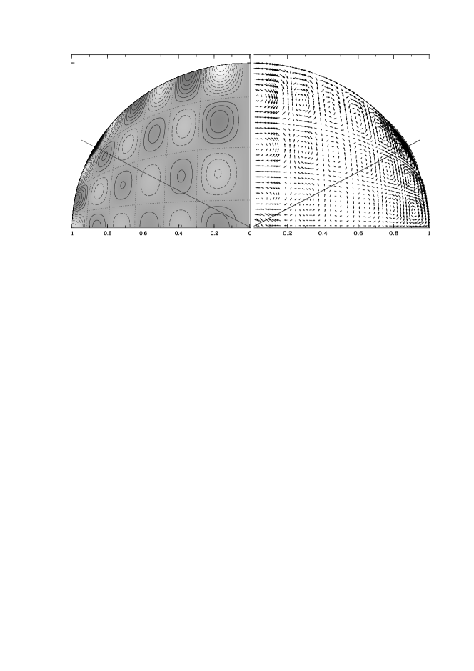
Figure 4.— A meridional look at the inertial-mode presented in Fig. 2. This mode is symmetric with respect to the equator, retrograde ($m=-2$), with $n_{1}=5$, $n_{2}=3$. The planet model has a density profile $\beta=1$. The left panel shows the Eulerian density perturbation ($\rho^{\prime}$), using both gray-scale and equidistant contours. Lighter regions (and dashed contours) stand for $\rho^{\prime}<0$, while darker regions (solid contours) represent $\rho^{\prime}>0$. The dotted curves indicate the $(x_{1},x_{2})$ coordinates. Counting the number of nodes along each coordinate, one recovers $n_{1}$ and $n_{2}$. The right panel shows the fluid velocity ($v_{r}$ & $v_{\theta}$ components only) in the rotating frame as arrows, with the size of the arrows proportional to $\sqrt{v}$. Notice that $v_{r}$ vanishes at the surface, as is required by the boundary condition (eq. [27]). Both the mode amplitude and the wave-vector remain relatively constant over much of the planet, but rise sharply toward the surface. This rise is most striking near the special angle $|\cos\theta|=\mu=0.4881$, marked here by straight lines.

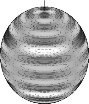
Figure 5.— Surface density perturbation ($\rho^{\prime}$) for the same mode ($m=-2,n_{1}=5,n_{2}=3$) as in Fig. 4. The short vertical stick marks the rotation axis. In both hemispheres, there is a latitudinal belt within which density perturbation attains the largest amplitude and varies with the steepest gradient. This lies around $|\cos\theta|=\mu$ and we call it the “singularity belt”. The surface pattern of the mode also discloses the quantum numbers: from the pole to the equator, there are $n_{1}$ nodal patches above the singularity belt, and $n_{2}$ nodes below it.

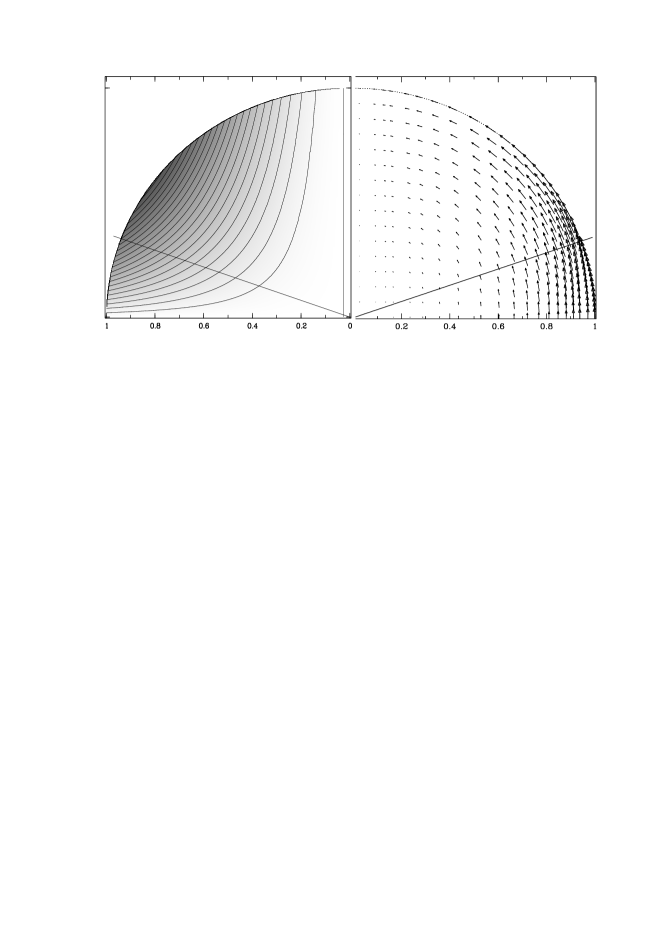
Figure 6.— As Fig. 4, except for a $m=-2$ R-mode. This mode has $\mu=1/(|m|+1)=0.3333$ and in our notation, $n_{1}=n_{2}=0$ and $\ell=|m|+1=3$. There is no internal nodal point and the radial velocity is zero everywhere. This mode exhibits odd symmetry toward the equator.

Figure 7.— Frequencies of even-parity, $|m|=2$ inertial-modes (shown here as ${\mbox{SIGN}}\mu$) as a function of wave-number $\lambda\sim 2(n_{1}+n_{2})$. Modes above the dotted line are prograde modes, and retrograde if below. These frequencies are obtained using a uniform density model but the overall features persist for more general models. Note the asymmetry between the frequencies of prograde and retrograde modes – this follows from equations (36) & (37).

Appendix A Ellipsoidal Coordinates

Bryan (1889) introduced a new set of coordinates under which the left-hand-side of equation (14) becomes separable. For any given density profile, the right-hand-side of the same equation is generally inseparable – however, for the two special cases of uniform and power-law density profiles (§2.2 and 2.3), the right-hand-side becomes separable and we can obtain (semi)-analytical solutions for the inertial-modes. This new set of coordinates allow us to obtain good approximate solutions for more general density profiles (§2.4).

We scale all length in the problem by the radius of the planet so that the Cartesian coordinates, $x$, $y$ and $z$, fall within the range of $(-1,+1)$. The new ellipsoidal coordinates $(x_{1},x_{2},\phi)$ are related to the Cartesian coordinates as

$$x = \left[{{(1-x_{1}^{2})(1-x_{2}^{2})}\over{1-\mu^{2}}}\right]^{1\over 2}\cos\phi,$$

$$y = \left[{{(1-x_{1}^{2})(1-x_{2}^{2})}\over{1-\mu^{2}}}\right]^{1\over 2}\sin\phi,$$

$$z = {{x_{1}x_{2}}\over{\mu}},$$ (A1)

with $x_{1}\in[\mu,1]$, $x_{2}\in[-\mu,\mu]$, and $\phi$ is the usual azimuthal angle with $\phi\in[0,2\pi]$. The cylindrical and spherical radii are given by

$$\varpi^{2} = x^{2}+y^{2}={{(1-x_{1}^{2})(1-x_{2}^{2})}\over{({1-\mu^{2}})}},$$

$$r^{2} = x^{2}+y^{2}+z^{2}=1-{{(x_{1}^{2}-\mu^{2})(\mu^{2}-x_{2}^{2})}\over{(1-\mu^{2})\mu^{2}}}.$$ (A2)

The Jacobian that relates the new coordinate system $(x_{1},x_{2},\phi)$ to the Cartesian $(x,y,z)$ is

$$\begin{array}[]{c}{\cal J}={\rm det}\left|\begin{array}[]{lll}{{\partial x}/{\partial x_{1}}}\hskip 7.22743pt&{{\partial x}/{\partial x_{2}}}\hskip 7.22743pt&{{\partial x}/{\partial\phi}}\\ {{\partial y}/{\partial x_{1}}}\hskip 7.22743pt&{{\partial y}/{\partial x_{2}}}\hskip 7.22743pt&{{\partial y}/{\partial\phi}}\\ {{\partial z}/{\partial x_{1}}}\hskip 7.22743pt&{{\partial z}/{\partial x_{2}}}\hskip 7.22743pt&{{\partial z}/{\partial\phi}}\\ \end{array}\right|={{x_{1}^{2}-x_{2}^{2}}\over{(1-\mu^{2})\mu}}\end{array}$$ (A7)

so the volume element $dx\,dy\,dz={\cal J}dx_{1}\,dx_{2}\,d\phi$.

Fig. 1 depicts the equi-distance curves of $(x_{1},x_{2})$ in a meridional plane, as well as the equi-distance curves of radius $r$ in the $x_{1}-x_{2}$ plane. In 3-D, surfaces of constant $x_{1}$ appear as co-axial cylinders around the $z$-axis (or prolate ellipsoids), while surfaces of constant $x_{2}$ resemble bandannas symmetrical with respect to the equator (or oblate ellipsoids). On the spherical surface, either $x_{1}$ or $|x_{2}|$ (or both) equals $\mu$ – we call the region where $x_{1}\approx|x_{2}|\approx\mu$ the ’singularity belt’, a region of special significance. Moreover, $x_{1}=1$ at the rotation axis and $x_{2}=0$ at the equator.

Partial differentiation with respect to $\varpi$, $z$ and $r$ can be expressed in the new coordinates as,

$$\left.{{\partial}\over{\partial\varpi}}\right|_{z} = \left.{{\partial x_{1}}\over{\partial\varpi}}\right|_{z}\left.{{\partial}\over{\partial x_{1}}}\right|_{x_{2}}+\left.{{\partial x_{2}}\over{\partial\varpi}}\right|_{z}\left.{{\partial}\over{\partial x_{2}}}\right|_{x_{1}}=-{{(1-\mu^{2})\varpi}\over{x_{1}^{2}-x_{2}^{2}}}\left(x_{1}{{\partial}\over{\partial x_{1}}}-x_{2}{{\partial}\over{\partial x_{2}}}\right)$$ (A8)

$$\left.{{\partial}\over{\partial z}}\right|_{\varpi} = \left.{{\partial x_{1}}\over{\partial z}}\right|_{\varpi}\left.{{\partial}\over{\partial x_{1}}}\right|_{x_{2}}+\left.{{\partial x_{2}}\over{\partial z}}\right|_{\varpi}\left.{{\partial}\over{\partial x_{2}}}\right|_{x_{1}}={{\mu}\over{x_{1}^{2}-x_{2}^{2}}}\left[x_{2}(x_{1}^{2}-1){{\partial}\over{\partial x_{1}}}-x_{1}(x_{2}^{2}-1){{\partial}\over{\partial x_{2}}}\right],$$ (A9)

$$\left.{{\partial}\over{\partial r}}\right|_{\theta} = \left.{{\partial r}\over{\partial z}}\right|_{\theta}\left.{{\partial}\over{\partial z}}\right|_{\varpi}+\left.{{\partial r}\over{\partial\varpi}}\right|_{\theta}\left.{{\partial}\over{\partial\varpi}}\right|_{z}=-{{(1-x_{1}^{2})x_{1}}\over{(x_{1}^{2}-x_{2}^{2})r}}{\partial\over{\partial x_{1}}}+{{(1-x_{2}^{2})x_{2}}\over{(x_{1}^{2}-x_{2}^{2})r}}{\partial\over{\partial x_{2}}}.$$ (A10)

Appendix B Making $\beta$ Models

We construct a hydrostatic model for a power-law density profile of the form $\rho=(1-r^{2})^{\beta}$ (eq. [39]). Any value of $\beta$ is allowed, in contrast to the polytrope case where the polytrope index has to be smaller than $5$.

For our numerical integration, we adopt $\ln\rho$ as the independent variable, and $\ln p$ and $M(r)$ as the variables. Here $p$ is pressure and $M(r)$ is the mass within radius $r$. The normal hydrostatic equations apply with the boundary conditions that at the center $M(r)=0$ and at the surface,

$$p={{2^{\beta}g_{\rm surface}}\over{\beta+1}}(1-r)^{\beta+1},.$$ (B1)

where surface gravity $g_{\rm surface}=GM(r=1)/r(r=1)^{2}$. This is obtained using $dp/dr=-\rho g$. We can then solve the boundary value problem to obtain the interior structure of such a model. Here, $r$ runs from $0$ to $1$ and the density scale is arbitrary.

References

- Abramowitz & Stegun (1972) Abramowitz, M. & Stegun, I. A. 1972, Handbook of Mathematical Functions (Handbook of Mathematical Functions, New York: Dover, 1972)
- Bryan (1889) Bryan, G. H. 1889, Philos. Trans. R. Soc. London, A180, 187
- Dintrans & Rieutord (2000) Dintrans, B. & Rieutord, M. 2000, A&A, 354, 86
- Goldreich & Soter (1966) Goldreich, P. & Soter, S. 1966, Icarus, 5, 375
- Greenspan (1968) Greenspan, H. P. 1968, The Theory of Rotating Fluids (The Theory of Rotating Fluids, Cambridge University Press,1968)
- Guillot et al. (2004) Guillot, T., Stevenson, D., Hubbard, W., & Saumon, D. 2004, in Jupiter eds. Bagenal et al., in press
- Lindblom & Ipser (1999) Lindblom, L. & Ipser, J. R. 1999, Phys. Rev. D, 59, 044009