Temporal evolution of magnetic molecular shocks

In the first paper of this series (Paper I) we computed time dependent simulations of multifluid shocks with chemistry and a transverse magnetic field frozen in the ions, using an adaptive moving grid.

In this paper, we present new analytical results on steady-state molecular shocks. Relationships between density and pressure in the neutral fluid are derived for the cold magnetic precursor, hot magnetic precursor, adiabatic shock front, and the following cooling layer. The compression ratio and temperature behind a fully dissociative adiabatic shock is also derived.

To prove that these results may even hold for intermediate ages, we design a test to locally characterise the validity of the steady state equations in a time-dependent shock simulation. Applying this tool to the results of Paper I, we show that most of these shocks (all the stable ones) are indeed in a quasi-steady state at all times, i.e. : a given snapshot is composed of one or more truncated steady shock. Finally, we use this property to produce a construction method of any intermediate time of low velocity shocks ($u<20$ kms^-1) with only a steady-state code. In particular, this method allows one to predict the occurrence of steady CJ-type shocks more accurately than previously proposed criteria.

1 Introduction

In a previous paper (Lesaffre et al. 2004, hereafter Paper I)(Lesaffre et al. (2004), we presented a numerical method to compute the time-dependent evolution of molecular shocks with a realistic cooling and chemistry in the presence of a transverse magnetic field. The use of a moving grid algorithm allowed us to reduce the number of zones and the computational time. However, the computation of the evolution of a stable shock from formation to steady-state still involves one or two days of CPU time on a 500 MHz workstation. Oscillating shocks require one week or two. This prevents the use of this code to fit shock parameters to observations.

On the other hand, steady-state codes give a fast answer (in one or two minutes) and include much richer physics. They have therefore been extensively used to interpret observed spectra. Nevertheless, steady-state codes have their limits. Observed magnetic molecular shocks may not be fully in steady-state yet, in which case they show a combination of C-type and J-type features. They might also be mildly or strongly unstable (Lim et al. 2002; Smith & Rosen 2003, and Paper I of this series), in which case a steady state model will have limited success.

However, different attempts have been made to circumvent these problems. In the field of shocks in supernovae remnants, Raymond et al. (1988) among others were successful in interpreting spectra with truncated steady J-shocks. Those models allowed them to account for incomplete recombination zones in a filament of the Cygnus loop. Chièze et al. (1998) discovered that the nascent magnetic precursor in a C-type shock was identical to a truncation of the steady state shock (for sufficiently late ages). Flower & Pineau des Forêts (1999) used this result to reproduce H₂ excitation diagrams in Cepheus A West.

The aim of this paper is to rigorously test the ideas of Raymond et al. (1988) and Flower & Pineau des Forêts (1999), by clarifying the relationship between time-dependent models and steady-state models. Indeed, we will show that time-dependence is within reach of steady state codes, as long as the shock is not subject to strong instabilities.

In Sect. 2 we study the stationary equations of magnetic shocks, and derive new analytical relations. Section 2 is independent of the other sections. Then, in Sect. 3, we assess the validity of the stationary approach by using the results of our fully hydrodynamical code (Paper I). In Sect. 4, we explain how to build time-dependent models of low velocity shocks with the only help of a steady-state code. We discuss our results in Sect. 5 and sum up our conclusions in Sect. 6.

2 Analytics of steady shocks

When the flow is in a steady state, time derivatives can be skipped in the steady frame. We derive here a few analytical relations valid along such steady flows.

2.1 Dynamical equations in a conservative form

We recall here the time-dependent monodimensional equations of multifluid hydrodynamics with a frozen transverse magnetic field. We put them in their conservative form :

$$\frac{\partial}{\partial t}(n_{j})+\frac{\partial}{\partial x}(n_{j}u_{\rm n}+J_{j})=R_{j}\mbox{ for $j$ neutral specie }$$ (1)

$$\frac{\partial}{\partial t}(n_{j})+\frac{\partial}{\partial x}(n_{j}u_{\rm c}+J_{j})=R_{j}\mbox{ for $j$ ionic specie }$$ (2)

$$\frac{\partial}{\partial t}(\rho_{\rm n}u_{\rm n})+\frac{\partial}{\partial x}(\rho_{\rm n}u_{\rm n}^{2}+p_{\rm n}+\pi_{\rm n})=F_{\rm c\rightarrow n}$$ (3)

$$\frac{\partial}{\partial t}(\rho_{\rm c}u_{\rm c})+\frac{\partial}{\partial x}(\rho_{\rm c}u_{\rm c}^{2}+p_{\rm c}+\pi_{\rm i}+\frac{B^{2}}{8\pi})=F_{\rm n\rightarrow c}$$ (4)

$$\frac{\partial}{\partial t}(\frac{1}{\gamma-1}p_{\rm n}+\frac{1}{2}\rho_{\rm n}u_{\rm n}^{2})+\frac{\partial}{\partial x}[u_{\rm n}(\frac{\gamma}{\gamma-1}p_{\rm n}+\frac{1}{2}\rho_{\rm n}u_{\rm n}^{2}+\pi_{\rm n})]$$

$$=\Lambda_{\rm n}+Q_{\rm i\rightarrow n}+Q_{\rm e\rightarrow n}+u_{\rm n}F_{\rm c\rightarrow n}-\frac{1}{2}u_{\rm n}^{2}M_{\rm n}$$ (5)

$$\frac{\partial}{\partial t}(\frac{1}{\gamma-1}p_{\rm i}+\frac{1}{2}\rho_{\rm i}u_{\rm c}^{2}+\frac{B^{2}}{8\pi})$$

$$+\frac{\partial}{\partial x}[u_{\rm c}(\frac{\gamma}{\gamma-1}p_{\rm i}+\frac{1}{2}\rho_{\rm i}u_{\rm c}^{2}+\pi_{\rm i}+\frac{B^{2}}{4\pi})]$$

$$=\Lambda_{\rm i}+Q_{\rm n\rightarrow i}+Q_{\rm e\rightarrow i}+u_{\rm c}F_{\rm n\rightarrow c}-\frac{1}{2}u_{\rm c}^{2}M_{\rm i}$$ (6)

$$\frac{\partial}{\partial t}(\frac{1}{\gamma-1}p_{\rm e}+\frac{1}{2}\rho_{\rm e}u_{\rm c}^{2})+\frac{\partial}{\partial x}[u_{\rm c}(\frac{\gamma}{\gamma-1}p_{\rm e}+\frac{1}{2}\rho_{\rm e}u_{\rm c}^{2})]$$

$$=\Lambda_{\rm e}+Q_{\rm n\rightarrow e}+Q_{\rm i\rightarrow e}-\frac{1}{2}u_{\rm c}^{2}M_{\rm e}$$ (7)

$$\frac{\partial}{\partial t}(B)+\frac{\partial}{\partial x}(u_{\rm c}B)=0$$ (8)

n, i, e, and c indices stand for neutrals, ions, electrons, and charges. $n_{j}$, $\rho$, $u$, $B$, $p$, and $\pi$ are respectively the number densities, mass densities, velocities, magnetic field, thermal and viscous pressures. $M$, $F$, $Q$ are the mass, momentum, and heat transfer rates. $\Lambda$ denotes radiative losses. $R_{j}$ stands for chemical rates, and $J_{j}$ for diffusive fluxes.

2.2 Steady state equations

Let us assume we are in a frame where the flow is in a steady state. We may then drop the $\frac{\partial}{\partial t}$ terms in equations 1-8. If we now integrate equations 1-8 along the $x$ coordinate, we link the state of the gas at one point $x$ in the shock to the state of the gas far upstream, i.e. to the entrance parameters of the shock (denoted with a 0 superscript in the following). We give here the result of such an integration in terms of conserved fluxes (dotted letters) through the steady region :

Mass flux :

$$\dot{M_{\rm n}}=\rho^{0}_{\rm n}u^{0}_{\rm n}=\rho_{\rm n}u_{\rm n}-\int_{0}^{x}M_{\rm n}{\rm d}x^{\prime}$$ (9)

$$\dot{M_{\rm c}}=\rho^{0}_{\rm c}u^{0}_{\rm c}=\rho_{\rm c}u_{\rm c}+\int_{0}^{x}M_{\rm n}{\rm d}x^{\prime}$$ (10)

Momentum flux :

$$\dot{P_{\rm n}}=\rho^{0}_{\rm n}(u^{0}_{\rm n})^{2}+p^{0}_{\rm n}$$

$$=\rho_{\rm n}u_{\rm n}^{2}+p_{\rm n}+\pi_{\rm n}-\int_{0}^{x}F_{\rm c\rightarrow n}{\rm d}x^{\prime}$$ (11)

$$\dot{P_{\rm c}}=\rho^{0}_{\rm c}(u^{0}_{\rm c})^{2}+p^{0}_{\rm c}+\frac{(B^{0})^{2}}{8\pi}$$

$$=\rho_{\rm c}u_{\rm c}^{2}+p_{\rm c}+\pi_{\rm i}+\frac{B^{2}}{8\pi}-\int_{0}^{x}F_{\rm n\rightarrow c}{\rm d}x^{\prime}$$ (12)

Energy flux :

$$\dot{E_{\rm n}}=u^{0}_{\rm n}(\frac{\gamma}{\gamma-1}p^{0}_{\rm n}+\frac{1}{2}\rho^{0}_{\rm n}(u^{0}_{\rm n})^{2})$$

$$=u_{\rm n}(\frac{\gamma}{\gamma-1}p_{\rm n}+\frac{1}{2}\rho_{\rm n}u_{\rm n}^{2}+\pi_{\rm n})-\int_{0}^{x}S_{\rm n}{\rm d}x^{\prime}$$ (13)

$$\dot{E_{\rm i}}=u^{0}_{\rm c}(\frac{\gamma}{\gamma-1}p^{0}_{\rm i}+\frac{1}{2}\rho^{0}_{\rm i}(u^{0}_{\rm c})^{2}+\frac{(B^{0})^{2}}{4\pi})$$

$$=u_{\rm c}(\frac{\gamma}{\gamma-1}p_{\rm i}+\frac{1}{2}\rho_{\rm i}u_{\rm c}^{2}+\pi_{\rm i}+\frac{B^{2}}{4\pi})-\int_{0}^{x}S_{\rm i}{\rm d}x^{\prime}$$ (14)

$$\dot{E_{\rm e}}=u^{0}_{\rm c}(\frac{\gamma}{\gamma-1}p^{0}_{\rm e}+\frac{1}{2}\rho^{0}_{\rm e}(u^{0}_{\rm c})^{2})$$

$$=u_{\rm c}(\frac{\gamma}{\gamma-1}p_{\rm e}+\frac{1}{2}\rho_{\rm e}u_{\rm c}^{2}+\pi_{\rm e})-\int_{0}^{x}S_{\rm e}{\rm d}x^{\prime}$$ (15)

where $S_{\rm n}$, $S_{\rm i}$, and $S_{\rm e}$ stand for the source terms in the right hand side of the conservative form of the total energy equations 1-8. We define $\Lambda=S_{\rm n}+S_{\rm i}+S_{\rm e}$ and we note that $\Lambda=\Lambda_{\rm n}+\Lambda_{\rm i}+\Lambda_{\rm e}$.

Magnetic flux :

$$\dot{B}=u^{0}_{\rm c}B^{0}=u_{\rm c}B$$ (16)

Integrals involve the source terms describing collisional, chemical, and thermal exchanges between different fluids, and radiative losses. The other terms describe the conservative phenomena that share mass, momentum, and energy between their available reservoirs (thermal, kinetic, viscous, magnetic…).

In each sector of a steady J or C shock, we will now get algebraic relations between the dominant conserved quantities. We tackle successively the following features, in the order in which a parcel of gas entering a magnetised shock would meet them :

• the cold magnetic precursor, in which the ion velocity is mainly decelerated, and friction starts to brake the neutrals,

• the hot magnetic precursor, in which the friction has brought the temperature to a sufficiently high level that H₂ cooling starts to play a dominant role (usually above neutral temperatures of 10³ K),

• the adiabatic front, in which viscosity in the neutrals converts their remaining kinetic energy into heat,

• the relaxation layer, in which the gas cools down, is compressed, and gets back to a thermal and chemical equilibrium.

Finally, we derive analytical properties of the atomic plateau that follows dissociative shock fronts.

2.2.1 Cold magnetic precursor

We assume here and in all the following that the ionisation fraction is very low :

$$\dot{M}=\dot{M_{\rm n}}+\dot{M_{\rm c}}=\rho_{\rm n}u_{\rm n}$$ (17)

Viscous, ram and thermal pressure of the charges also are negligible compared to neutrals and magnetic pressure. Furthermore, since this region is far from the adiabatic shock front, neutral viscosity can safely be neglected as well. The total momentum flux is then :

$$\dot{P}=\dot{P_{\rm n}}+\dot{P_{\rm c}}=\rho_{\rm n}u_{\rm n}^{2}+p_{\rm n}+\frac{B^{2}}{8\pi}$$ (18)

If the temperature of the neutrals stays low, radiative losses can be neglected, and the total energy flux is :

$$\dot{E}=\dot{E_{\rm n}}+\dot{E_{\rm c}}=u_{\rm n}(\frac{\gamma}{\gamma-1}p_{\rm n}+\frac{1}{2}\rho_{\rm n}u_{\rm n}^{2})+u_{\rm c}\frac{B^{2}}{4\pi}$$ (19)

Finally, conservation of the magnetic flux through the steady region gives :

$$\dot{B}=Bu_{\rm c}$$ (20)

We thus get 4 equations with 5 unknowns $\rho_{\rm n}$, $u_{\rm n}$, $p_{\rm n}$, $B$, and $u_{\rm c}$. One variable can then be chosen to get expressions for all the others. For example, $p_{\rm n}$ is solution of a quadratic whose coefficients depend on the shock parameters and the neutral density $\rho_{\rm n}$ :

$$p_{\rm n}^{2}\frac{2\pi}{\dot{B}^{2}}\frac{\dot{M}^{2}}{\rho_{\rm n}^{2}}\frac{\gamma^{2}}{(\gamma-1)^{2}}$$

$$+p_{\rm n}[1-\frac{2\pi\dot{M}}{\dot{B}^{2}\rho_{\rm n}}\frac{2\gamma}{\gamma-1}(\dot{E}-\frac{1}{2}\frac{\dot{M}^{3}}{\rho_{\rm n}^{2}})]$$

$$-\dot{P}+\frac{\dot{M}^{2}}{\rho_{\rm n}}+\frac{2\pi}{\dot{B}^{2}}(\dot{E}-\frac{1}{2}\frac{\dot{M}^{3}}{\rho_{\rm n}^{2}})^{2}=0$$ (21)

As another example, $u_{\rm n}$ is solution of a quadratic whose coefficients depend on the shock parameters and $u_{\rm c}$ :

$$\frac{\gamma+1}{2(\gamma-1)}\dot{M}u_{\rm n}^{2}-\frac{\gamma}{\gamma-1}(\dot{P}-\frac{\dot{B}^{2}}{8\pi u_{\rm c}^{2}})u_{\rm n}+\dot{E}-\frac{\dot{B}^{2}}{4\pi u_{\rm c}}=0$$ (22)

These relations hold up to the point above which radiative losses cannot be neglected anymore (they would hold as well in C-shocks upstream this point). In our simulations (Paper I), this corresponds to the point where $T_{\rm n}>10^{3}$ K. The gas then enters the hot magnetic precursor, where H₂ cooling becomes dominant.

2.2.2 Hot magnetic precursor

In this part of the magnetic precursor, ram pressure is directly transferred into radiation via friction. There is no more increase in the thermal pressure. Therefore, the neutral thermal pressure becomes very quickly negligible against magnetic pressure. It also remains negligible against ram pressure in the rest of the magnetic precursor. This leads to the following reduced set of equations :

$$\begin{array}[]{lcl}\dot{M}&=&\rho_{\rm n}u_{\rm n}\\ \dot{P}&=&\rho_{\rm n}u_{\rm n}^{2}+\frac{B^{2}}{8\pi}\\ \dot{B}&=&Bu_{\rm c}\end{array}$$ (23)

We can derive from this a relation between the speeds of neutrals and charges that is valid in magnetic precursors (or C-shocks) downstream the point where $|\int_{0}^{x}\Lambda{\rm d}x|$ dominates over $u_{\rm n}\frac{\gamma}{\gamma-1}p_{\rm n}$ (usually, when $T_{\rm n}$ is greater than 10³ K) :

$$u_{\rm n}=\frac{1}{\dot{M}}(\dot{P}-\frac{\dot{B}^{2}}{8\pi u_{\rm c}^{2}})$$ (24)

This last equation is complementary to equation 22. These equations provide a powerful way to test if the magnetic field compression is correctly treated in a multifluid code.

2.2.3 Adiabatic shock front

In the shock front, the viscous pressure $\pi_{\rm n}$ is one additional unknown. We will therefore assume that we know the magnetic field $B_{\rm p}$ at the end of the magnetic precursor, as well as the amount of energy radiated away in the precursor $\dot{E}_{\rm p}=\int_{\mbox{\small precursor}}\Lambda{\rm d}x^{\prime}$. Since the shock front is very tenuous, it is fair to assume that neither the magnetic field nor the integrated radiative losses will vary across it.

We can then define the new conserved fluxes for this region :

$$\begin{array}[]{lcl}\dot{P}^{\prime}&=&\dot{P}-\frac{B_{\rm p}^{2}}{8\pi}\\ \dot{E}^{\prime}&=&\dot{E}+\dot{E}_{\rm p}\end{array}$$ (25)

Four equations then combine together :

$$\begin{array}[]{lcl}\dot{M}&=&\rho_{\rm n}u_{\rm n}\\ \dot{P}^{\prime}&=&\rho_{\rm n}u_{\rm n}^{2}+p_{\rm n}+\pi_{\rm n}\\ \dot{E}^{\prime}&=&u_{\rm n}(\frac{\gamma}{\gamma-1}p_{\rm n}+\frac{1}{2}\rho_{\rm n}u_{\rm n}^{2}+\pi_{\rm n})+u_{\rm c}\frac{B_{\rm p}^{2}}{8\pi}\\ \dot{B}&=&u_{\rm c}B_{\rm p}\\ \end{array}$$ (26)

Here, we explicitly deduce the pressure in terms of the density :

$$p_{\rm n}=(\gamma-1)(\frac{1}{2}\frac{\dot{M}^{2}}{\rho_{\rm n}}-\dot{P}^{\prime}+\frac{\dot{E}^{\prime}-\dot{B}B_{\rm p}/8\pi}{\dot{M}}\rho_{\rm n})$$ (27)

We are not aware of any previous analytic expression relating pressure to density throughout an adiabatic shock front, even in the absence of magnetic fields. This relation is useful to test a code in a shock front.

In addition, the post-shock velocity $u_{\rm n}$ can be calculated by setting $\pi_{\rm n}=0$ in equations LABEL:adequ, which gives the following quadratic equation :

$$\dot{M}\frac{\gamma+1}{2}u_{\rm n}^{2}-\gamma\dot{P}^{\prime}u_{\rm n}+(\gamma-1)(\dot{E}^{\prime}-\dot{B}B_{\rm p}/8\pi)=0$$ (28)

Without magnetic field and energy losses, this quadratic gives the post-shock velocity and hence the usual compression factor in an adiabatic shock. The same kind of reasoning will also provide us with analytic predictions in dissociative shock fronts (see 2.3).

2.2.4 Relaxation layer

Here, radiative losses are not negligible anymore, and the equation of conservation of energy is left aside. But outside the shock front, viscous pressures are negligible, so we only need to make an assumption about the magnetic field. Since we neglect the thermal and ram pressure of the charges, the momentum conservation of the charges yields :

$$\frac{B^{2}}{8\pi}=\dot{P_{\rm c}}+\int_{0}^{x}F_{\rm n\rightarrow c}{\rm d}x^{\prime}$$ (29)

For low shock velocities, the last integral is dominated by the magnetic precursor, where most of the ion deceleration occurs, and $B=B_{\rm p}$ is also a correct approximation in the relaxation layer. We are then left with two equations :

$$\begin{array}[]{lcl}\dot{M}&=&\rho_{\rm n}u_{\rm n}\\ \dot{P}^{\prime}&=&\rho_{\rm n}u_{\rm n}^{2}+p_{\rm n}\\ \end{array}$$ (30)

$p_{\rm n}(\rho_{\rm n})$ follows easily :

$$p_{\rm n}=\dot{P}^{\prime}-\frac{\dot{M}^{2}}{\rho_{\rm n}}$$ (31)

Note that the intersection of this relation with the thermal equilibrium relation $p_{\rm n}(\rho_{\rm n})$ gives the final steady post-shock conditions. Similarly, the intersection of the algebraic equations in two adjacent sectors of the shock gives the physical conditions at the transition between the two regions.

In cases of high shock velocities (greater than 30 kms^-1 for the models in Paper I), a recoupling of the velocities of charges and neutrals may happen in the relaxation layer, which builds up an additional magnetic pressure. After the recoupling zone, we can assume that $u_{\rm n}=u_{\rm c}$ :

$$\begin{array}[]{lcl}\dot{M}&=&\rho_{\rm n}u_{\rm n}\\ \dot{P}&=&\rho_{\rm n}u_{\rm n}^{2}+p_{\rm n}+\frac{B^{2}}{8\pi}\\ \dot{B}&=&Bu_{\rm n}\end{array}$$ (32)

$p_{\rm n}(\rho_{\rm n})$ follows easily :

$$p_{\rm n}=\dot{P}-\frac{\dot{M}^{2}}{\rho_{\rm n}}-\frac{\dot{B}^{2}}{8\pi\dot{M}^{2}}\rho_{\rm n}^{2}$$ (33)

At the high density end of the relaxation layer, the total pressure is dominated by magnetic pressure. This prevents the gas to be compressed while it cools down, and leads to much lower compression factors. The final state of the gas in this case corresponds to the steady isothermal compression factor calculated in the case of magnetic field coupled to the gas (see Draine & McKee 1993, equation 2.19a).

2.3 Adiabatic dissociative shock

In an adiabatic dissociative shock, energy losses can still be accounted for by conserved quantities since thermal energy of the gas is used to dissociate H₂, i.e. converted into internal energy. We then have :

$$\begin{array}[]{lcl}\dot{E}&=&u_{\rm n}(\frac{\gamma}{\gamma-1}p_{\rm n}+\frac{1}{2}\rho_{\rm n}u_{\rm n}^{2}+\pi_{\rm n})+\int_{0}^{x}R^{\rm d}_{{\rm H}_{2}}Q{\rm d}x^{\prime}\end{array}$$ (34)

where $Q$ = 4.48 eV is the binding energy of the H₂ molecule and $R^{\rm d}_{{\rm H}_{2}}$ is the local dissociation rate. The integral term is related to the change in the flux of H₂ molecules by :

$$\int_{0}^{x}R^{\rm d}_{{\rm H}_{2}}Q{\rm d}x^{\prime}=Q(0.5-f(x))\frac{\dot{M}x_{\rm H}}{\mu_{\rm H}}$$ (35)

where $f$ is the fractional abundance of H₂ by number relative to $n_{\rm H}$ (initially $f$ = 0.5), $x_{\rm H}$ is the (fixed) elemental hydrogen mass fraction, and $\mu_{\rm H}$ is the mass of one hydrogen atom.

For more clarity, we neglect here the effects of the charged fluid, but it would be straightforward to include the magnetic pressure and radiative effects using primed shock parameters like in the previous subsections. We then obtain a modified version of equations LABEL:adequ, including the H₂ dissociation energy :

$$\begin{array}[]{lcl}\dot{M}&=&\rho_{\rm n}u_{\rm n}\\ \dot{P}&=&\rho_{\rm n}u_{\rm n}^{2}+p_{\rm n}+\pi_{\rm n}\\ \dot{E}&=&u_{\rm n}(\frac{\gamma}{\gamma-1}p_{\rm n}+\frac{1}{2}\rho_{\rm n}u_{\rm n}^{2}+\pi_{\rm n})+(1-2f)\frac{\dot{M}Qx_{\rm H}}{2\mu_{\rm H}}\end{array}$$ (36)

Unfortunately, we do not have a fixed relation between $p_{\rm n}$ and $\rho_{\rm n}$ as in the non-dissociative case, because the H₂ fraction $f$ varies across the front and adds to the unknowns. But the conditions at the end of the front can be found if one sets $\pi_{\rm n}=0$ and $f=f^{*}$ where $f^{*}$ is the H₂ fraction at the end of the shock. So doing, we get an equation similar to relation 28 :

$$\dot{M}\frac{\gamma+1}{2}u_{\rm n}^{2}-\gamma\dot{P}u_{\rm n}+(\gamma-1)(\dot{E}-(1-2f^{*})\frac{\dot{M}Qx_{\rm H}}{2\mu_{\rm H}})=0$$ (37)

We simplify this equation by assuming the high Mach number regime, for which $\dot{P}=u^{0}\dot{M}$ and $\dot{E}=\frac{1}{2}(u^{0})^{2}\dot{M}$ :

$$\frac{\gamma+1}{2}u_{\rm n}^{2}-\gamma u_{\rm n}u^{0}+\alpha\frac{\gamma-1}{2}(u^{0})^{2}=0$$ (38)

where we defined $\alpha=1-(1-2f^{*})\frac{Qx_{\rm H}}{(u^{0})^{2}\mu_{\rm H}}$. $1-\alpha$ measures the relative decrease in energy flux through the shock front due to H₂ dissociation. In a non-dissociative shock, $\alpha=1$ since $f^{*}=0.5$. $\alpha$ reaches a minimum of $0.74$ for a fully dissociative shock ($f^{*}=0$) just above the dissociation limit $u^{0}=u_{\rm d}\simeq 30$ kms^-1, and tends to one again for very high shock speeds (where the H₂ dissociation energy becomes negligible compared to the kinetic flux).

The compression factor through such a shock can now be computed :

$$C=\frac{u^{0}}{u_{\rm n}}=\frac{\rho_{\rm n}}{\rho^{0}}=\frac{\gamma+\sqrt{\gamma^{2}(1-\alpha)+\alpha}}{(\gamma-1)\alpha}$$ (39)

The usual compression $C_{\rm a}=\frac{\gamma+1}{\gamma-1}$ is recovered when $\alpha=1$. $C=5.8$ for $\gamma=5/3$ and $\alpha=0.74$.

We can get a simple expression for the temperature of the atomic plateau ($f^{*}=0$) if we neglect the post-shock ram pressure (so that $p_{\rm n}=\rho^{0}(u^{0})^{2}$). This is only 20% accurate for the compression factor obtained (we use $\gamma=5/3$) :

$$T_{\rm p}=\frac{\mu_{\rm p}}{{\rm k}_{\rm B}}(u^{0})^{2}\alpha$$ (40)

where $\mu_{\rm p}$ is the mean molecular weight in the plateau. $T_{\rm p}$ is hence nearly quadratic in the entrance velocity for strong shocks.

The knowledge of the compression factor, along with the assumption of steadiness of the adiabatic front provides us with the velocity of the front relative to the piston in the adiabatic phase of a dissociative shock front :

$$v=u/(C-1)$$ (41)

2.4 Validation of the analytical results on examples

We verified the analytical relations derived above by comparing with numerical magnetic shock simulations from Paper I.

First, we find that the temperature and density of the atomic plateau are well predicted by the formulae 40 in most dissociative shocks. This was expected, since the width of the adiabatic shock is so small that it is very likely to be in a steady state : the sound crossing time of this feature is much shorter than the time of variation of the entrance shock speed. In addition, in strongly oscillating shocks (weakly dissociative case of Paper I), the maximum expansion of the front, corresponding to the adiabatic, fully dissociative phase, coincides with the velocity given by equation 41 (see Fig. 4d of Paper I).

We also verified the relations predicted for non-dissociative shocks. As an example, in Fig. 1, we check the relations 22 and 24 against the final steady-state of a C-type shock (diamonds). The agreement is very good, confirming that magnetic compression is correctly treated in the code.

Figure 1: Steady state analytic relations between the velocities of neutrals and charges are compared to an overlaid steady C-shock (diamonds). The parameters of the shock are $u=20$ kms^-1, $n=10^{4}\leavevmode\nobreak\$cm^-3 and $b=0.1$, time is $t=10^{5}$ yr. The velocities in the shock frame are computed using a velocity of the shock front of 0.13 kms^-1, inferred from Fig. 3d of Paper I.

Finally, in figure 2 we plot in diamonds the state of the gas for the same shock in a snapshot at $t=100$ yrs, i.e. well prior to steady (C-type) state. We overlay the algebraic relations previously derived for the various shock regions. The agreement turns out to be very good. This comforts us in the ability of the code to reproduce the conservation equations. It also points out the fact that steady equations may well be valid to describe a shock at early times, even though it has not reached its final steady-state. It is to address the domain of validity of this “quasi-steady” approximation that we set up the technique and tests described in the next section.

Figure 2: Steady state analytic relations between pressure and mass density are compared to an overlaid future C-shock (diamonds). The parameters of the shock are $u=20$ kms^-1, $n=10^{4}\leavevmode\nobreak\$cm^-3 and $b=0.1$, time is $t=10^{2}$ yr. The additional necessary parameters $B_{\rm p}$ and $\dot{E}_{\rm p}$ are read in the shock model at the end of the precursor (they are not fitted).

3 Validity of the quasi-steady assumption in time-dependent shocks

In this section we develop a method to characterise the local steady velocity for each variable separately, and we use it to test the ”steadiness” of various shock regions in the simulations of Paper I.

3.1 Local steady velocities and quasi-steady state

Consider $y$, one of the $N+6$ state variables that enter the set of equations 1-8. Its evolution equation in the frame of the piston can be cast in the following form :

$$\frac{\partial y}{\partial t}+\frac{\partial(uy)}{\partial x}=s$$ (42)

where $u=u_{\rm n}$ or $u_{\rm c}$ is the velocity of the fluid associated with $y$, and $s$ is a term that does not depend on the reference frame.

We define the local steady velocity $v_{y}$ for variable $y$ as : the velocity of a reference frame in which the time derivative in the evolution equation vanishes. Hence :

$$\frac{\partial}{\partial x}[(u-v_{y})y]=s$$ (43)

When $y$ does not involve a velocity, i.e. does not depend on the reference frame, a direct expression follows for the velocity $v_{y}$ :

$$v_{y}=[\frac{\partial(uy)}{\partial x}-s]/\frac{\partial y}{\partial x}.$$ (44)

One has to be more careful when $y$ depends on $u$. For example, in the case $y=\rho u$, $v_{y}$ is given implicitly by the following quadratic equation :

$$v_{y}^{2}\frac{\partial\rho}{\partial x}-2v_{y}\frac{\partial y}{\partial x}+\frac{\partial(uy)}{\partial x}=s$$ (45)

The expression 44 is singular when $\frac{\partial y}{\partial x}=0$. This can easily be understood : if the profile of $y$ is flat, any velocity will do. It is therefore crucial to take into account the finite numerical precision when trying to evaluate $v_{y}$ with these expressions. Indeed, roundoff errors can make the gradient of $y$ non zero even in places where it should be.

Finally, expressions 44 and 45 yield a way of characterising the “steadiness” of the flow. At a given position $x$, if $v_{y}$ does not depend on $y$, then there is indeed a frame moving at a velocity $v(x)$ in which none of the variables is changing in time. Furthermore, if this velocity is constant throughout an extended region, then this whole region is moving “en-bloc” at velocity $v$ and can be modelled with a truncated steady-state model. We say that this region is in a quasi-steady state.

3.2 Validity of the quasi-steady state in time-dependent shocks

For a selection of time steps of each of the dynamical models that we simulated in Paper I, we computed the steady velocities $v_{y}$ in each zone for each variable $y$.

We evaluated the numerical noise in the following way : we computed the change $\delta v_{yy^{\prime}}$ in the steady velocity $v_{y}$ when each variable $y^{\prime}$ was changed by 10^-4 in relative value (corresponding to our guess for the numerical precision). We then estimated the numerical noise $\sigma_{y}$ on variable $y$ by :

$$\sigma_{y}^{2}=\sum_{y^{\prime}}(\delta v_{yy^{\prime}})^{2}$$ (46)

The noise-weighted mean steady velocity over all variables of a subset $S$ was then computed in each zone, as well as the corresponding numerical noise $\sigma_{\rm noise}$ :

$$v=(\sum_{y\in S}v_{y}/\sigma_{y}^{2})/(\sum_{y\in S}1/\sigma_{y}^{2})$$ (47)

$$\sigma_{\rm noise}^{2}=1/(\sum_{y\in S}1/\sigma_{y}^{2})$$ (48)

For charges and neutral momentum, both roots of quadratic 45 where included. But for reasons that will become clear in the next subsections, magnetic field was excluded from this mean. Finally, the variance of individual $v_{y}$ values about this mean velocity and the corresponding $\chi^{2}$ were estimated :

$$\sigma^{2}=[\sum_{y\in S}(v_{y}-v)^{2}/\sigma_{y}^{2}]/(\sum_{y\in S}1/\sigma_{y}^{2})$$ (49)

$$\chi^{2}=\frac{1}{\#S}\sigma^{2}/\sigma_{\rm noise}^{2}=\frac{1}{\#S}\sum_{y\in S}(v_{y}-v)^{2}/\sigma_{y}^{2}$$ (50)

where $\#S$ is the number of variables in the subset $S$.

If the numerical noise is well estimated, a value of $\chi^{2}\simeq 1$ indicates that the dispersion of invidual $v_{y}$ values is consistent with local numerical noise, i.e. that there may exist a common steady velocity for all the variables of the subset $S$ at that position. Regions where this is fulfilled and $v$ is constant are the quasi-steady regions for the set $S$.

A less strict criterion can be chosen for the local steadiness if we think of the ratio $v/\sigma$ as a “signal to noise” : even if $\chi^{2}$ is high, it may be possible that the ratio $v/\sigma$ is high. In this case, the steady velocities corresponding to different variables are not equal, but they are close to one another : therefore, a common steady velocity $v$ is a good approximation.

It turns out that we compute very low values of $\chi^{2}$ in quite a few zones. This indicates that the numerical precision we have in these zones is far better than our estimate of $10^{-4}$. We hence rather use the criterion based on the ratio $v/\sigma$ and define the quasi-steady regions as the regions with a constant velocity $v$ and a good “signal to noise” ratio.

The subset of variables $S$ on which the averages are computed should be the whole set of variables. However, the last section of this paper needs only that the dynamically important variables be in a quasi-steady state. Therefore we present here the results for a subset $S$ including the temperatures of the three fluids, the four velocities (roots of equation 45 for $y=\rho_{\rm n}u_{\rm n}$ and $y=\rho_{\rm c}u_{\rm c}$), He, H₂, H₂O, CO and OH densities. We do not include the magnetic field in magnetised shocks, because its steady velocity differs from the other variables as we will show in the next section. We also did the calculation for $S$ including all the variables but the magnetic field, and found that it did not change the general conclusions : the signal to noise ratio is slightly less good, and a few zones are not quasi-steady anymore because of marginal chemical species having a different steady velocity than the bulk of the variables.

We summarise the results of our investigation in the next two subsections, devoted respectively to non-magnetised and magnetised shocks.

3.2.1 J-type shocks ($B$=0)

Non-dissociative J-type shocks

Figure 3 shows the $\chi^{2}$ as well as $v$ with error bars $\pm\sigma$ in each zone of a typical snapshot of a non-dissociative J-type shock. The adiabatic front and relaxation layer show a good “signal to noise” ratio and a flat steady velocity. On the contrary, the pre-shock zones show a huge dispersion around the steady velocity, expected from the homogeneity of the medium there. The fact that we retained both velocities from expression 45 does not alter the results, because the numerical errors on velocities are actually much larger than for the other variables.

Figure 3: We plot the $\chi^{2}$ values and steady velocities for each variables of $S$ in each zone of snapshot $t=200$ years for the shock with parameters $b=0$, $n=10^{4}\leavevmode\nobreak\$cm^-3, and $u=20$ kms^-1. Each dot represents the steady velocity of one variable computed thanks to expressions 44 and 45. The error bars are $v\pm\sigma$ evaluated zone per zone on these values. We indicate the computational domains associated to the adiabatic front and the relaxation layer of the shock.

We find that all of our non-dissociative J-type shocks are in a quasi-steady state from the adiabatic phase to the steady phase (only the initial formation of the shock front is not quasi-steady). Therefore, a snapshot of such a shock will always coincide with the truncated structure of a J-type steady state.

In Paper I, we plotted the trajectory of the point of maximum ratio of viscous over thermal pressure (see Fig. 1b). We compute here the average steady velocity $v$ over the whole structure of the shock (trimmed from the pre-shock values) at various times and overlay it over this trajectory in Fig. 4. Error bars show the good consistency of the test, and the correspondence of $v$ with the velocity at which the viscous shock front moves away from the piston.

Note that the entrance velocity in the shock is not the upstream velocity $u$ of the fluid towards the piston, but rather $u^{0}=u+v$. Hence, the entrance shock speed for the truncated steady shock is evolving in time. In Sect. 4, we present a way to reconstruct this evolution.

Figure 4: Trajectory and velocity away from the piston of the J-shock with parameters $b=0$, $n=10^{4}\leavevmode\nobreak\$cm^-3, and $u=20$ kms^-1 (from Paper I). Overlaid diamonds are the steady velocities $v$ averaged over all variables and all zones, for each snapshot analysed.

Dissociative J-type shocks

On the contrary, dissociative shocks are almost never in a quasi-steady state. For weakly dissociative velocities, we could not come up with a coherent picture. This was expected, since these shocks are highly unstable with large bouncing oscillations between a fully dissociative expansion phase and a non-dissociative recoil phase (Paper I). Partly ionised shocks are less unstable. We illustrate their behaviour with a typical example shown in Fig. 5. The adiabatic front is generally in a quasi-steady state with velocity roughly equal to the velocity of the viscous maximum, but the dispersion is much higher than for non-dissociative shocks. The first plateau that follows (with H ionisation and Lyman cooling) is not at all in a quasi-steady state : the dispersion is huge and the mean velocity is not even constant. The second plateau (H recombination) seems rather quasi-steady, but with a velocity much lower than the adiabatic shock front. This warns us that steady-state diagnostics may be hopeless for weakly non-dissociative shocks, and that we have to be cautious for partly ionising shocks.

Figure 5: Same as Fig. 3, but for a partly ionising shock of parameters $b=0$, $n=10^{4}\leavevmode\nobreak\$cm^-3, and $u=40$ kms^-1 at time $t=220$ years. Here, the scale of the plot is linear, so that the dispersion is in fact much greater than for the non-dissociative shocks, even in the second plateau.

3.3 CJ-type and C-type shocks

Figure 6 shows $v$ with error bars $\pm\sigma$ in each zone of an early snapshot of a non-dissociative C-type shock. The shock then has a composite CJ structure made of a magnetic precursor, followed by a non-dissociative adiabatic front and a relaxation layer. We find that the magnetic precursor is in a quasi-steady state with a high steady velocity. This is in agreement with the remark of Chièze et al. (1998). At the very end of the magnetic precursor, the large dispersion in steady velocities is due to the fact that two different steady velocities coexist among the variables. Following this, the adiabatic front and relaxation layer appear to be in a quasi-steady state, but with a much lower velocity than the magnetic precursor. However, strictly speaking, it is not a real quasi-steady state, as the steady velocity for the magnetic field remains equal to the high steady velocity of the magnetic precursor.

Figure 6: Same as Fig. 3, but for time $t=100$ years of the future C-shock with $b=0.1$, $n=10^{4}\leavevmode\nobreak\$cm^-3, and $u=20$ kms^-1. We also show the steady velocity for the magnetic field.

Figure 7 shows that the two steady velocities (relaxation layer and precursor) correspond well to the velocities of the viscous maxima of neutrals and charges determined by time-derivation of their trajectory. As time evolves, the velocity of the magnetic precursor and that of the relaxation layer get closer to one another, and finally coincide after the J-front has disappeared. The C-type structure is then in a quasi-steady state as a whole.

In principle, one should then be able to model an early age of a low velocity C shock by combining a truncated C-type model with a truncated J-type model (in which the magnetic field is treated appropriately). The problem is a bit more complex than in the J-type case because we need now to determine two different truncation distances and two sets of entrance parameters, but we will show in Sect. 4.2 that it is possible to solve.

This picture holds for all shocks with magnetic field, as long as there is no dissociation or ionisation plateau. In the case of dissociative velocities, the same problems described in the previous subsection arise in the corresponding features of the relaxation layer.

Figure 7: Same as Fig. 4, but for a C-shock of parameters $b=0.1$, $n=10^{4}\leavevmode\nobreak\$cm^-3 and $u=20$ kms^-1. Curves plot the trajectory and velocity of the neutral (solid) and charged (dashed) viscous fronts. Diamonds are the quasi-steady velocities of the relaxation layer and adiabatic front. Triangles are the quasi-steady velocities of the magnetic precursor.

This picture is the same for all magnetic shocks. The only difference between CJ-type and C-type is whether or not the J-front has disappeared when the steady velocities of the relaxation layer and the magnetic precursor converge. From this remark, we will obtain in Sect. 4.2.1 a way to assess if a low velocity shock will eventually become a steady CJ-type shock.

4 Time-dependent constructions of shocks at early times

Here, we derive methods of reconstruction of time-dependent shocks using truncated steady models. Those constructions will be meaningful only for the shocks in which the quasi-steady state has been validated at all times, although they can in principle be realised in any shock. Due to their different complexities, we treat successively the case of non-dissociative J-type shocks and non-dissociative magnetised shocks.

4.1 Non-dissociative J-type shocks

Section 3.2.1 has shown that the whole structure of non-dissociative J-type shocks is at all times quasi-steady. One may then safely fit truncated steady models to observations. The fitted parameters would be the entrance parameters in the shock frame and the truncation distance. But one would then like a method to relate these parameters to the parameters of the shock in the piston frame, and to the age of the shock. Conversely, one would like to build at will a snapshot of a shock of given age and parameters (in the piston frame), with the only help of a steady state code. We come up with such a procedure in the following.

A steady-state code provides us with the steady profile of any variable in the frame of the shock front for a given set of entrance parameters $(u^{0},n)$. Say, the steady velocity $u_{\rm s}(u^{0},n;x)$, where $x$ is the distance from the shock front. If we are given an inflow speed and density $(u,n)$ in the frame of the piston and a time $t$, the problem is to find what is the entrance velocity $u^{0}$ at the same time $t$ in the frame of the shock front as well as the corresponding distance $r$ between the shock front and the piston.

To help set up the notations in both frames of the shock and of the piston, we sketched in Fig. 8 the different lengths and velocities involved.

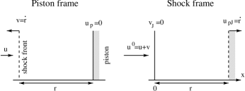
Figure 8: Schematical view of a J-type shock in the piston frame and in the shock frame.

At any given time, velocities in the shock frame are found by adding $v=\dot{r}$ to velocities in the piston frame. The entrance shock speed is then :

$$u^{0}=u+\dot{r},$$ (51)

while the velocity at the piston — which must be null in the piston frame — is, in the J-shock frame :

$$u_{\rm s}(u^{0},n;r)=\dot{r}.$$ (52)

These relations combine to give an implicit equation linking $\dot{r}$ to $r$ :

$$\dot{r}=u_{\rm s}(u+\dot{r},n;r)$$ (53)

Furthermore, in a quasi-steady state, mass conservation requires that $u_{\rm s}(u^{0},n;r)\times C=u^{0}$, i.e. $\dot{r}=v=u/(C-1)$ where $C$ is the compression factor at the piston. From the adiabatic phase ($C=4$) to the steady state ($C<<1$), the speed $v$ of the front thus decreases from $\frac{1}{3}u$ to nearly $0$. Therefore, if the steady state code provides $u_{\rm s}(u^{0},n;r)$ for a range of velocities $u<u^{0}<\frac{4}{3}u$, the equation 53 is an implicit ordinary differential equation straightforward to integrate up to time $t$ with initial conditions $r=0$ and $\dot{r}=\frac{1}{3}u$. Actually, an interpolation between a few steady models might be sufficient to get accurate results.

Conversely, if the problem is to recover the time from a steady model truncated at distance $R$, we only have to integrate equation 53 backward in time up to the point where $r=0$ and compute $t=\int_{0}^{R}\frac{1}{\dot{r}}{\rm d}r$.

High compression factor approximation :

For high compression factors, the final $\dot{r}$ is small enough to be neglected with respect to $u$, which makes the computation even easier. The integral yielding the age is dominated by the very low velocities, which are also the most recent ones. Therefore, we only need one steady state model $u_{\rm s}(x)=u_{\rm s}(u,n,B;x)$. The age of such a truncated shock is simplified in the following way.

$$t=\int_{0}^{R}\frac{1}{u_{\rm s}}{\rm d}x$$ (54)

In this last expression, one recognises the flow time across the shock. Since for strongly radiative shocks, the compression factor rises very quickly, this approximation is valid even for very young ages. For example, the shock of parameters $b=0$, $n=10^{4}$ cm^-3, and $u=20$ kms^-1 has a compression factor of 10 at as early as $t=1$ year (see Fig. 4).

4.2 Non-dissociative magnetised shocks

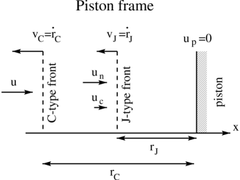
Figure 9: Schematical view of an early magnetised shock in the piston frame.

The analysis of Sect. 3 showed that low-velocity magnetised shocks are composed of two quasi-steady regions : a magnetic precursor, and a non dissociative J-type feature. In faster shocks, where the entrance velocity in the J-type feature is dissociative, the J-type structure is not in a quasi-steady state, although the magnetic precursor is. We thus restrict our analysis to the non-dissociative cases.

In principle, one should then be able to model a snapshot of such a shock by gluing together two truncated steady C and J models. The problem is to determine the entrance parameters and lengths of each of the two shock features, for a given time $t$ and a given set of parameters $(u,n,B)$ in the piston frame. A rigorous construction method is outlined below.

In the following, $r_{\rm C}$ and $r_{\rm J}$ denote respectively the distance of the fronts of the C-type and the J-type features with respect to the piston (see Fig. 9). Variables computed in the reference frame of the C-type feature are denoted with C subscripts. Variables in the J-type feature frame are specified with J subscripts. Entrance parameters in the shocks have a 0 superscript.

Now, let us assume that we know the positions $r_{\rm C}$ and $r_{\rm J}$ at current time $t$. To solve for their evolution, we need to find equations that will determine $\dot{r}_{\rm C}$ and $\dot{r}_{\rm J}$.

The entrance velocities in the C-type feature are simply:

$$\begin{array}[]{lcl}u_{\rm nC}^{0}&=&\dot{r}_{\rm C}+u\\ u_{\rm cC}^{0}&=&\dot{r}_{\rm C}+u\\ n^{0}_{\rm C}&=&n\\ B^{0}_{\rm C}&=&B\end{array}$$ (55)

The steady-state code for the C-type feature then provides us with the entrance values of velocities, densities, and magnetic field at the position of the J-front, $x=r_{\rm C}-r_{\rm J}$. After a suitable change of reference frame for the velocities, they determine the entrance parameters in the J-type shock :

$$\begin{array}[]{lcl}u_{\rm nJ}^{0}&=&\dot{r}_{\rm J}-\dot{r}_{\rm C}+u_{\rm nC}(u+\dot{r}_{\rm C},n,B;r_{\rm C}-r_{\rm J})\\ u_{\rm cJ}^{0}&=&\dot{r}_{\rm J}-\dot{r}_{\rm C}+u_{\rm cC}(u+\dot{r}_{\rm C},n,B;r_{\rm C}-r_{\rm J})\\ n_{\rm nJ}^{0}&=&n_{\rm nC}(u+\dot{r}_{\rm C},n,B;r_{\rm C}-r_{\rm J})\\ n_{\rm cJ}^{0}&=&n_{\rm cC}(u+\dot{r}_{\rm C},n,B;r_{\rm C}-r_{\rm J})\\ B_{\rm J}^{0}&=&B_{\rm C}(u+\dot{r}_{\rm C},n,B;r_{\rm C}-r_{\rm J})\end{array}$$ (56)

The steady-state J-shock must then be integrated. A multifluid treatment is necessary, since $u_{\rm n}$ and $u_{\rm c}$ at the entrance of the J-front are different. Furthermore, a special treatment of magnetic field compression is necessary, since Sect. 3.3 showed that the steady velocity for the magnetic field in the J-type feature is not $\dot{r}_{\rm J}$, but remains the same as in the magnetic precursor, namely $v_{B}=\dot{r}_{\rm C}$. It means that the product of $B$ with the velocity of charges computed in the frame of the C shock remains constant through the J-type feature :

$$B\times(u_{\rm cJ}-\dot{r}_{\rm J}+\dot{r}_{\rm C})=B_{\rm C}^{0}\times u_{\rm cC}^{0}$$ (57)

Therefore, the evolution of the J-type feature depends not only on the entrance parameters determined above but also on $\dot{r}_{\rm C}-\dot{r}_{\rm J}$.

As in the non-magnetic case, the derivatives $\dot{r}_{\rm C}$ and $\dot{r}_{\rm J}$ are then determined by stating that both charges and neutrals have to be at rest near the piston, i.e., in the frame of the J-front :

$$\begin{array}[]{lcl}\dot{r}_{\rm J}&=&u_{\rm nJ}(u_{\rm nJ}^{0},u_{\rm cJ}^{0},n_{\rm nJ}^{0},n_{\rm cJ}^{0},B_{\rm J}^{0},\dot{r}_{\rm C}-\dot{r}_{\rm J};r_{\rm J})\\ \dot{r}_{\rm J}&=&u_{\rm cJ}(u_{\rm nJ}^{0},u_{\rm cJ}^{0},n_{\rm nJ}^{0},n_{\rm cJ}^{0},B_{\rm J}^{0},\dot{r}_{\rm C}-\dot{r}_{\rm J};r_{\rm J})\\ \end{array}$$ (58)

We thus get two independent implicit equations for $\dot{r}_{\rm J}$ and $\dot{r}_{\rm C}$. Numerical techniques to solve these equations still need to be designed, but should not be too hungry in CPU time.

4.2.1 Final steady state: C or CJ ?

We have now a means of computing the time evolution of a magnetised shock with only a steady-state code. One should then be able to integrate it from initial conditions $r_{\rm J}=r_{\rm C}=0$ up to the steady state where $\dot{r}_{\rm J}$ and $\dot{r}_{\rm C}$ are equal constants. If during the evolution the entrance velocity in the J-shock $u_{\rm nJ}^{0}$ becomes subsonic, then one should stop the integration because the J-shock disappears, and the remaining sound wave propagates through the structure until a stationary C-type structure is obtained. If $u_{\rm nJ}^{0}$ stays supersonic when $\dot{r}_{\rm J}$ and $\dot{r}_{\rm C}$ are equal constants, then the result is a CJ-type shock steady-state. Hence, one is forced to integrate over time $\dot{r_{\rm J}}$ and $\dot{r_{\rm C}}$ given implicitly by equations 58 to know what is the final steady-state corresponding to a given set of parameters $(u,n,B)$.

However, one could also think about solving equations 56 and 58 for given arbitrary values of the final front velocity $v_{\rm f}=\dot{r}_{\rm J}=\dot{r}_{\rm C}$. The result would be a series of physically consistent steady CJ-type states, each characterised by a different distance $r_{\rm C}-r_{\rm J}$. Only one of these is selected by the time evolution but, if the entrance parameters $(u,n,B)$ are allowed to evolve in time, it might be possible that several (or even all) of these final states can be realised. The final state would then depend on the evolution history of the entrance parameters.

In fact, a very easy way to exhibit one of those CJ-type steady-states would be to use a multifluid steady-state code, and trigger the viscous dissipation in the neutral at a given position $r_{\rm C}-r_{\rm J}$ where the neutral velocity is still supersonic.

4.2.2 Low velocity, high compression factor approximations

For all the low velocity cases encountered in our simulations, we noted that after one year of time, the velocity of the charges was already almost brought to rest at the end of the magnetic precursor. This approximation yields the following equation :

$$\dot{r}_{\rm C}=u_{\rm cC}(u+\dot{r}_{\rm C},n,B;r_{\rm C}-r_{\rm J})$$ (59)

which implicitly gives the velocity $\dot{r}_{\rm C}$. The velocity $\dot{r}_{\rm J}$ can then be retrieved by solving the first equation of the set 58.

Just like for the J-type shocks, high magnetic compression factors will lead to $\dot{r}_{\rm C}$ negligible before $u$, and will facilitate the integration of equation 59. In this case, and if in addition $r_{\rm J}<<r_{\rm C}$, the age of the shock is given by :

$$t=\int_{0}^{r_{\rm C}-r_{\rm J}}\frac{1}{u_{\rm cC}}{\rm d}x$$ (60)

which is the flow time of the charges across the magnetic precursor.

5 Discussion

The analytic relations we found make good benchmarks for testing codes. In addition, they might provide some theoretical basis for further investigation of the properties of these shocks in the parameter space.

The quasi-steady state analysis of shocks opens a new field of possibilities for the steady-state codes. We compare hereafter our method to previously used algorithms, and sketch possible extensions of our method.

5.1 Comparison with previous work

Our quasi-steady state analysis of J-shocks justifies the use of truncated steady-state J-shocks by Raymond et al. (1988). We provide more theoretical basis to link the true age of the shock to the truncation distance used.

Flower & Pineau des Forêts (1999) and Le Bourlot et al. (2002) use simple algorithms to produce mixed C-type and J-type features to mimic time-dependent magnetised shocks. Le Bourlot et al. (2002) greatly improved the method used by Flower & Pineau des Forêts (1999) since they keep the multifluid treatment of the flow through the relaxation layer. They just switch on viscosity in the neutral fluid when they encounter a sonic point. The present analysis gives a less heuristic way to know at which point the viscosity should be switched on, and Paper I has already shown that it can be way upstream a sonic point. Furthermore, we specify that a change of velocity frame has to be done at the end of the magnetic precursor, except for the magnetic field equation. Finally, we state where the J-type structure has to be truncated for a given time $t$.

Our new method should therefore lead to more accurate results, and will allow the construction of much earlier phases of magnetised shocks. It shows as well that the criterion used by Le Bourlot et al. (2002) to assess whether steady-states will be of CJ-type (occurrence of a sonic point in the neutral fluid) has to be revised. CJ-type steady states may in fact occur at lower speeds, when velocity recoupling between neutral and charges enhances magnetic compression near the piston, and slows down the precursor to the expansion speed of the J-front.

5.2 Possible extensions of the method

First, let us point out that the time-dependent construction method derived here relies only on the quasi-steady state assumption for a limited number of variables, namely velocities, densities, and magnetic field. For example, if a set of chemical species can be identified to have no impact on the dynamics, they can be skipped in the process of building the truncation radii, and computed only in the last resort.

Following the same idea, if non-dynamically important species happen to be non quasi-steady, they can be post-processed in parallel to the quasi-steady time-evolution with a Lagrangian code.

Here we present an algorithm for two kinematic flows (charges and neutrals), but the same method may be implemented for more flows. Especially, the treatment of charged grains could be envisaged, in relation to the questions raised by Ciolek & Roberge (2002) and Flower & Pineau des Forêts (2003). The only caveat is that we do not yet have a consistent check for the validity of the quasi-steady assumption.

Finally, our algorithm is straightforward to apply with slowly changing input conditions $(u,n,B)$ in the piston frame. One has only to bear in mind that if these parameters change over time-scales much shorter than the crossing time scale of the shock, then the quasi-steady assumption is very likely to be violated.

5.3 Limitations of our method

Our algorithm is based upon the quasi-steady state assumption. However, it will give results with any shock. One problem is that we still have no other way to assess the validity of the steady-state assumption than computing the time-dependent evolution with a fully hydrodynamical code.

We encountered several cases where this assumption was not realised. Strongly unstable shocks like the weakly dissociative ones violate strongly this assumption. Fortunately, they seem to happen for a very restricted range of parameters. Partly ionising shocks are very slightly unstable, and are closer to meet the quasi-steady state assumption. They might therefore be accounted for by our algorithm. Finally, quite a few magnetised shocks have unstable entrance velocities for the J-shock only at early times, and are afterwards quasi-steady at all times. These shocks may be as well within reach of our algorithm if one is ready to skip the early evolution. However, one should always be cautious when a plateau with dissociated molecules appears in a steady-state computation.

An other situation where the quasi-stationary assumption may be strongly violated is the case where a dynamically important chemical specie is not in a quasi-steady state. This might happen when a dominating cooling agent varies on very short time scales. Furthermore, diffusion effects, if they turn out to be important, will destroy the quasi-steady state as well.

6 Conclusions

In a companion paper (Paper I), we produced fully time-dependent numerical simulations of molecular shocks.

In the present paper, we derived new analytical relations valid at quasi-steady state, and successfully checked them on our simulations. These relations provide useful benchmarks to test existing and future multifluid codes.

In light of the simulations run in Paper I, we investigated carefully the validity of the quasi-steady state approximation. It was found that at all times stable shocks could be accounted for by truncated steady models. We point out as well that caution has to be kept regarding the use of steady-state models for dissociative velocities.

Finally, we produced a new algorithm based on the quasi-steady state assumption. With only a steady-state code, this method is able to compute time-dependent snapshots of shocks in the presence or not of a magnetic field. Therefore, it brings time-dependence within the reach of steady models, and should greatly improve the diagnostics of observed molecular shocks. Furthermore, it provides a way of assessing the CJ nature of a magnetised shock. Finally, this algorithm can be extended to many shocks other than molecular, provided that the quasi-steady state approximation is validated.