Temporal evolution of magnetic molecular shocks

We present time-dependent 1D simulations of multifluid magnetic shocks with chemistry resolved down to the mean free path. They are obtained with an adaptive moving grid implemented with an implicit scheme. We examine a broad range of parameters relevant to conditions in dense molecular clouds, with preshock densities $10^{3}$ cm${}^{-3}<n<10^{5}$ cm^-3, velocities $10$ kms^-1$\leavevmode\nobreak\ <u<40$ kms^-1, and three different scalings for the transverse magnetic field : $B=0,0.1,1\leavevmode\nobreak\ \mu$G$\times\sqrt{n/{\rm cm}^{-3}}$.

We first use this study to validate the results of Chièze, Pineau des Forêts & Flower (1998), in particular the long delays necessary to obtain steady C-type shocks, and we provide evolutionary time-scales for a much greater range of parameters.

We also present the first time-dependent models of dissociative shocks with a magnetic precursor, including the first models of stationary CJ shocks in molecular conditions. We find that the maximum speed for steady C-type shocks is reached before the occurrence of a sonic point in the neutral fluid, unlike previously thought. As a result, the maximum speed for C-shocks is lower than previously believed.

Finally, we find a large amplitude bouncing instability in J-type fronts near the H₂ dissociation limit ($u\simeq 25-30\leavevmode\nobreak\$kms^-1), driven by H₂ dissociation/reformation. At higher speeds, we find an oscillatory behaviour of short period and small amplitude linked to collisional ionisation of H. Both instabilities are suppressed after some time when a magnetic field is present.

In a companion paper, we use the present simulations to validate a new semi-analytical construction method for young low-velocity magnetic shocks based on truncated steady-state models.

1 Introduction

Today, essentially all observational diagnostics of shocks are based on steady state models. Indeed, the steady state form of the monodimensional equations of hydrodynamics for these shocks is an ordinary differential equation. Therefore, computation of such models can encompass the luxury of details involved in the thermal, magnetic and chemical richness of the interstellar medium. Hollenbach & McKee (1979, 1980, 1989) describe the destruction and reformation of molecules in very strong jump (hereafter J-type) shocks, after having studied their radiative precursor (Shull & McKee 1979). Mullan (1971) discovered that high magnetic fields can transfer kinetic energy to thermal energy in a continuous manner (C-type shocks). Draine (1980), Draine et al. (1983), and Roberge & Draine (1990) describe the multifluid nature of these shocks. In a series of papers Flower & Pineau des Forêts (1985, 1986, 1995); Le Bourlot et al. (2002); Flower et al. (2003); Flower & Pineau des Forêts (2003) carefully examine the relevant chemistry, and in a more general way, all collisional interactions between the charged and neutral fluids. They point out the strong influence of chemistry on the magnetic precursor, carefully address the energy losses linked with this chemistry, and stress the need to follow the level populations of H₂ along the flow. H₂ is indeed one of the most efficient coolants, and therefore one of the most powerful diagnostics. A good review of the steady state J-type and C-type models can be found in Draine & McKee (1993). All these studies assume a purely transverse magnetic field frozen in the ions. Other authors (Pilipp et al. 1990; Pilipp & Hartquist 1994; Caselli et al. 1997; Wardle 1998) have investigated the dynamical role of the grains as well as the effect of oblique magnetic fields. For high pre-shock densities, they showed that the drift velocity had been underestimated, producing a significant rise in the maximum temperature. They also discovered that rotation of the magnetic field could bring one of the charged fluids at rest in the shock frame.

Time-dependent studies of dense shocks in one dimension have focused separately on three points. The first one is the oscillatory instabilities due to the temperature dependence of the cooling of the gas (Chevalier & Imamura 1982; Gaetz et al. 1988; Strickland & Blondin 1995; Walder & Folini 1996; Lim et al. 2002; Smith & Rosen 2003). The second one is the early evolution of multifluid shocks, which is found to involve a combination of C and J shock fronts (Pineau des Forêts et al. 1997; Smith & Mac Low 1997; Chièze et al. 1998). Pineau des Forêts et al. (1997) and Chièze et al. (1998) include non-equilibrium cooling and chemistry in the fluids, with a degree of details comparable to steady state models. They prove that in low ionised magnetised media, the steady state could be reached only after very late ages (up to a few times 10⁵ yr), far greater than the variation time scales of shock driving sources. The third point is the dynamical effects of grains, which is beginning to be included in time-dependent studies (Ciolek & Roberge 2002; Falle 2003).

Chièze, Pineau des Forêts & Flower (1998) used a time stretching method to resolve the sharp J-fronts in time-dependent magnetised shocks. However, their method did not allow to resolve non-viscous fronts (e.g. H₂ reformation regions), and could introduce synchronisation problems. To overcome both limitations, we have developed a new moving grid algorithm which allows one to resolve discontinuities down to the mean free path. Although we do not include the treatment of grain dynamics to remain consistent with Chièze et al. (1998), we note that our numerical scheme already provides the required framework to solve the problems mentioned by Falle (2003), as it is implicit with very high resolution. As such, it is the first algorithm able to model time-dependent multifluid dissociative shocks.

In this paper, we use our code to validate the evolutionary behaviour and time scales obtained with the ”anamorphosis” method of Chièze et al. (1998), and to extend their range of shock parameters to cover the denser conditions encountered in protostellar jets and molecular clouds, including dissociative and partly ionising shocks. We (1) compute the evolution time-scales of these shocks, and interpret physically their behaviour, (2) find that stationary CJ shocks are obtained before the occurence of a sonic point in the shock frame and are thus more frequent than previously thought, (3) describe two types of oscillations driven by chemistry that were not identified previously.

In Sect. 2, we briefly present our numerical model, with the improvements made compared to Chièze et al. (1998). Section 3 describes the results and compares them to previous work. Section 4 discusses the limitations of our method and Sect. 5 summarises our conclusions.

2 Numerical and physical inputs

2.1 Numerical scheme

2.1.1 Time-step integration

We use a fully non-linear implicit scheme for time integration. The implicitation parameter is set equal to 0.55 : that way, we combine a quasi order 2 accuracy in time with an unconditional stability of the scheme. We use a Van-Leer advection scheme. The relative variations of the variables is kept under 5% at each time-step. We reproduce classical tests such as the Sod’s shock tube, Rankine-Hugoniot relations, and Sedov explosion with a 0.3% accuracy.

More details can be found in Lesaffre (2002).

We solve for the same equations as Chièze et al. (1998), although the hydrodynamics and chemistry are now solved simultaneously. This amounts to a number of 33 chemical equations, 2 momentum equations, 4 energy equations and one equation for the moving mesh all coupled together. Solving for the chemistry without splitting it from the hydrodynamics helps numerical convergence, but has a computational cost, since the Jacobian matrix is far heavier to be inverted. In a few cases, the code stalled because a proper convergence of the Newton-Raphson iterations required a time step much too small.

2.1.2 Adaptive grid

Chemistry encompasses an extensive range of time scales, down to times as short as a few mean collision times of the particles. When this range of time scales is coupled with hydrodynamics, it generates a full range of spatial scales, down to a few mean free paths.

To achieve this extremely high resolution where needed, we use the moving grid algorithm designed by Dorfi & Drury (1987). We define the delay time parameter of the grid as the sound crossing time of the smallest zone. Our resolution function combines three arguments : the gradient of the neutral temperature, the gradient of the ionic temperature, and the maximum of all chemical gradients.

Thanks to this method, we were able to resolve all shocks and chemical fronts with a total number of zones as low as 100, without having to resort to the anamorphosis method of Chièze et al. (1998). The present code can safely handle two or more sharp features like a strong shock followed by a molecular reformation region, or a shock, a contact discontinuity and a reverse shock. The natural viscosity is used in the shock fronts, resulting in a viscous spread of typically $10^{-3}$ pc/($n_{\rm H}$.cm³) resolved with about 10 zones.

2.1.3 Diffusion

We consider diffusion for the chemical species, based on a Fick law with a diffusion length equal to the local mean free path $\lambda_{\rm d}=1/\sigma n_{\rm H}$ where $\sigma=10^{-15}\leavevmode\nobreak\$cm² is the molecular cross section, and $n_{\rm H}$ is the numerical density of hydrogen nuclei. This is motivated by the fact that in regions where molecules are reforming, the fluid velocities are usually very low. The reformation times of the molecules would then lead to an unrealistically thin front. This diffusion term ensures that the front has at least a width of the order of the mean free path.

2.2 Physical inputs

2.2.1 Chemistry

The network comprises around 120 reactions involving 33 different species (including electrons). It is the same network as Chièze et al. (1998) with a few additional (or updated) reactions :

• collisional dissociations of H₂ by e^- (Flower et al. 1996), H, H₂, He, and streaming ions (Wilgenbus et al 2000).

• collisional ionisation of H by e^- (Le Bourlot et al. 2002).

• updated H₂ formation on grains : for the sticking coefficient, we use expression (4) of Hollenbach & Salpeter (1971) calibrated by Buch & Zhang (1991) and Masuda et al. (1998).

To compute the energy transfers and coolings due to chemical reactions, we properly track the fluid to which each species belong. This is critical especially for endothermic reactions like collisional ionisation of H.

2.2.2 Atomic and molecular cooling

We use refined versions of all the atomic and molecular coolings used by Chièze et al. (1998), with the addition of H cooling.

At each time-step, we compute the level population of C (4 levels), C⁺ (4 levels) and O (5 levels) excited by e^-, H, He, and H₂. Collisional excitation coefficients are taken from Mendoza (1983); Hayes & Nussbaumer (1984); Monteiro & Flower (1987); Hollenbach & McKee (1989); Lavalley (2000). Lyman $\alpha$ cooling is taken from Flower et al. (1996), and cooling due to radiative recombination of H is from Spitzer (1978) (case B). We properly track the energy lost by each fluid, depending on the collider.

We consider cooling by H₂ (Le Bourlot et al. 1999), OH (Hollenbach & McKee 1979), CO and H₂O (Neufeld & Kaufman 1993). Since the latter authors provide data for excitation of CO by H₂ only, we assumed the same excitation coefficients for H-CO collisions. The optical depth parameter is computed in the static approximation, with a distance scale corresponding to $A_{\rm v}$ = 10 mag.

2.3 Parameter space and initial conditions

The three parameters $n$ (number density of hydrogen nuclei), $u$ (initial velocity), and $B$ (initial ambient magnetic field) characterise a simulation. We replace $B$ by the parameter $b$, setting $B=b(n.$cm${}^{3})^{\frac{1}{2}}\leavevmode\nobreak\ \mu$G. Typical conditions in the interstellar medium correspond to $b=1$. But as we consider only the transverse component of the field, $b$ can take values between 0 and 1. We combine $n=10^{3}$, $10^{4}$, $10^{5}$ cm^-3, $u=10$, 20, 30, 40 kms^-1, and $b=0$, 0.1, 1 and produce a grid of 36 different simulations. To test the dynamical instability that we observed in dissociative cases, we ran two additional cases with $b=0$, $u=25$ kms^-1, $n=10^{4}$ and $10^{5}$ cm^-3. The abundances of He, C, O, and Fe nuclei relative to $n_{\rm H}$ are the following : He=0.1 ; C=1.7$\leavevmode\nobreak\ 10^{-4}$ ; O=4.25 $10^{-4}$ ; Fe=1.8$\leavevmode\nobreak\ 10^{-7}$.

We use a piston-like protocol. The initial conditions of the simulation box are homogeneous, in thermal and chemical equilibrium with a density corresponding to a given $n_{\rm H}=n$. The transverse magnetic field is uniform, equal to $B$. All interfaces of the cells in the simulation have a velocity $u$, except the last one, which is a fixed reflexive boundary. The moving grid algorithm allows us to begin with a very small simulation box of a few mean free paths (typically 30). We make the left border of the box continuously flee the shock front. That way, the adiabatic shock is always fully resolved. The simulation is stopped when the box is too large and the resolution of sharp fronts cannot be supported any more by the algorithm. This occurs when the dynamical range of length scales is greater than typically a billion.

3 Results

3.1 Final steady-states and trajectories in the piston frame

Table 1 summarises the final steady-state of each model as a function of the initial parameters $b$, $n$, and $u$. When $b=0$, all flows evolve to stable J-type shocks, except at intermediate velocities for which we find strong or moderate undamped oscillations. When $b$ is finite, the flow generally evolves to a steady C-type shock. At sufficiently low $b$ or high $u$, however, a strong J shock in the neutrals persists behind the continuous magnetic precursor, and a steady CJ-type shock is obtained. Figures 1-2-3 show the thermal and chemical structure of typical shocks in their final J, CJ and C-type steady-state. Figures 4-5 show intermediate states of J-shocks with higher entrance velocities.

Fig. 1 : J-shock	Fig. 2 : CJ-shock	Fig. 3 : C-shock

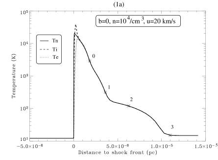
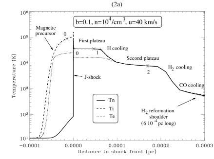
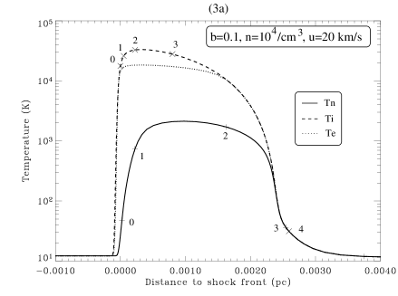
Figure 1: Stationary structure at $t=2\leavevmode\nobreak\ 10^{3}$ yr and shock trajectories of a J-type shock with $n=10^{4}\leavevmode\nobreak\$cm^-3, $u=20$ kms^-1, and $b=0$. (a) Thermal structure : temperatures of the neutrals, ions and electrons. The crosses on the curve are the points where the flow time computed in the frame of the shock is equal to $10^{n}$ yr, $n$ being the number indicated near the cross. ’+’ signs stand for neutrals and ’x’ for charges. (b) Cooling structure : magnitude of the main cooling processes. (c) Chemical structure : abundance relative to hydrogen nuclei of species of interest. (d) Shock trajectory : Position (thick curve) and velocity (thin curve) of the J-front against time, in the frame of the piston. Fig. 2. Same as Fig. 1 for a steady CJ-type shock with $n=10^{4}\leavevmode\nobreak\$cm^-3, $u=40$ kms^-1, and $b=0.1$, at $t=2\leavevmode\nobreak\ 10^{3}$ yr. The dashed curve in (d) plots the position of the C-precursor against time. Fig. 3. Same as Fig. 2 for a steady C-type shock with $n=10^{4}\leavevmode\nobreak\$cm^-3, $u=20$ kms^-1, and $b=0.1$, at $t=10^{5}$ yr.

Fig. 4 : weakly dissociative J-shock	Fig. 5 : partly ionising J-shock

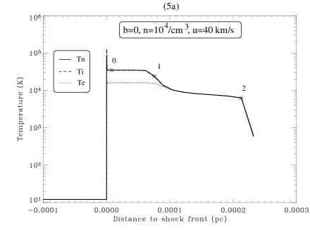
Figure 4: Same as Fig. 1 for a weakly dissociative J-shock of parameters $n=10^{5}\leavevmode\nobreak\$cm^-3, $u=25$ kms^-1, $b=0$ at $t=50$ yr. In panel (d), the thick solid line is the trajectory of the shock in a simulation with a reduced network of 8 species. The simulation with the whole network is plotted in a thick dashed line, up to the point where it stalled. Fig. 5. Same as Fig. 1 for a partly ionising J-shock of parameters $n=10^{4}\leavevmode\nobreak\$cm^-3, $u=40$ kms^-1, $b=0$ at $t=220$ yr.

At the bottom of these figures, we also plot the shock trajectories, i.e. the positions as a function of time of the C precursor and the J front (defined as the zones with maximum ratio of viscous to thermal pressure in the ionic and neutral fluids, respectively). We also plot their corresponding propagation velocity $v$ away from the piston, obtained by differentiating with respect to time, and smoothing with a median filter (20 time steps of width). This avoids spurious high velocities due to change in the zone number.

Even at intermediate times, $v$ for stable J-type fronts is found to obey the steady-state relation $v=u/(C-1)$ where $C$ is the neutral fluid compression factor at the piston. In the initial adiabatic phase, $v=u/3$ ($C=4$ for $\gamma=5/3$). It then decreases during the cooling phase, down to a steady value when thermal equilibrium is reached in the post-shock gas. These three phases can be very clearly seen in Fig. 1d. For the C-type precursor, the initial velocity corresponds to the ion magnetosonic speed. $v$ then decreases as $u/(C-1)$ where $C$ is now the magnetic compression factor (see Lesaffre et al. 2004, hereafter Paper II). At early times, the J-type feature of a magnetised shock behaves like the same shock without magnetic field, as neutrals and ions are still decoupled. Thus, the J-front propagates much slower than the C-front, which allows the magnetic precursor to grow. In the steady C-type case, the J-front velocity eventually catches up with the C-front due to the softening of its entrance conditions. In the steady CJ-type case, the C-front velocity is forced to slow down to the J-front value by early effective recoupling between the neutrals and the magnetic field through their collisional interactions with ions, and the precursor growth is halted.

3.2 Time scales and length scales

Table 1 gives, next to the final state of the shock (J, CJ, or C), the time scales in years taken to reach steady state. It includes in parentheses the width (in pc) of the steady-state shock structure (we give the length of both C and J components for CJ-type shocks).

We compared a time evolution sequence for parameters $b=1$, $n=10^{3}$, and $u=10$ kms^-1 to Fig. 6 of Chièze et al. (1998). We find a very good agreement, though we use a very different method of integration, that cooling processes have been strongly refreshed to account for dissociative shocks, and that our resolution is higher at both shocks and relaxation layer. The method used by Chièze et al. (1998) to recover the time is hence validated.

In particular, we confirm the long time scales to steady C-type shocks found by these authors, of the order of the ion crossing time scale, and their weak dependence on the magnetic field for $0<b\leq 1$. We add here (see Table 1) that these time scales are roughly inversely proportional to the density, as expected from the cooling time scales, and that there is no significant change with respect to the velocity, except when dissociative and non-dissociative velocities are compared (see also Fig. 4 of Le Bourlot et al. 2002, for example ). The length scales of the shocks which actually dissociate molecules are longer than the non-dissociating ones by a factor of 5-10, due to the fact that H₂ is a very efficient coolant.

$b=0$	$n=10^{3}\leavevmode\nobreak\$cm-3		$n=10^{4}\leavevmode\nobreak\$cm-3		$n=10^{5}\leavevmode\nobreak\$cm-3
$u$	$t$ (yr)	size (pc)	$t$ (yr)	size (pc)	$t$ (yr)	size (pc)
$10$ kms-1	J=104	(10-4)	J=2 103	(2.5 10-5)	J=2 102	(6 10-6)
$20$ kms-1	J=104	(5 10-5)	J=2 103	(10-5)	J=2 102	(4 10-6)
$25$ kms-1			J=5 102	(1.5 10-5)	Bouncing
					A=150	(2.2 10-4)
$30$ kms-1	J=104	(4 10-5)	Bouncing		Oscillating
			A=700	(8 10-4)
			o=100	(5 10-5)	o=40	(5 10-5)
$40$ kms-1	Oscillating		J=2 102	(2.5 10-4)	J=40	(2 10-5)
	o=650	(4 10-4)	o’=40	(3 10-5)	o’=2.5	(2 10-6)

$b=0.1$	$n=10^{3}\leavevmode\nobreak\$cm-3		$n=10^{4}\leavevmode\nobreak\$cm-3		$n=10^{5}\leavevmode\nobreak\$cm-3
$u$	$t$ (yr)	size (pc)	$t$ (yr)	size (pc)	$t$ (yr)	size (pc)
$10$ kms-1	C=105	(2 10 -2)	C=104	(3 10-3)	C=1.5 103	(4 10-4)
$20$ kms-1	C=105	(2 10 -2)	C=104	(3 10-3)	C=1.5 103	(4 10-4)
$30$ kms-1	C=105	(2 10 -2)	C$>$700		CJ=102	(C=2 10-5)
			A’=700	(8 10-4)		(J=3 10-4)
			o’=150	(5 10-5)	o=20	(10-5)
$40$ kms-1	CJ=5 103	(C=6 10-5)	CJ=250	(C=10-5)	CJ=40	(C=10-4)
		(J=$5\leavevmode\nobreak\ 10^{-3}$)		(J=10-3)		(J=10-4)
	o=500	(3 10-4)	o=25	(3 10-5)	o=3	(3 10-6)

$b=1$	$n=10^{3}\leavevmode\nobreak\$cm-3		$n=10^{4}\leavevmode\nobreak\$cm-3		$n=10^{5}\leavevmode\nobreak\$cm-3
$u$	$t$ (yr)	size (pc)	$t$ (yr)	size (pc)	$t$ (yr)	size (pc)
$10$ kms-1	C=105	(2 10 -1)	C=1.3 104	(4 10 -2)	C=1.5 103	(6 10-3)
$20$ kms-1	C=105	(2 10 -1)	C=1.3 104	(4 10 -2)	C=1.5 103	(5 10-3)
$30$ kms-1	C=105	(2 10 -1)	C=104	(3 10 -2)	C=1.5 103	(4 10-3)
			A’=1000	(10-3)	A’=500	(4 10-4)
			o’=150	(5 10-5)	o’=15	(1 10-6)
$40$ kms-1	C=4 104	(10 -1)	CJ=103	(C=6 10-3)	CJ=2 102	(C=10-3)
	A’=4000	(3 10-3)		(J=5 10-2)		(J=10-2)
	o’=600	(10-4)	o’=25	(3 10-5)	o’=2.5	(10-6)

Table 1: For each run, we provide the final steady-state of each shock (J, CJ, C) followed by the time scale in years at which steadiness is achieved. The total width of the shock at this point (in pc) is given in parentheses (in the case of CJ-type shocks, J is the length of the relaxation layer, and C is the length of the magnetic precursor). C$>700$ indicates that a J-front is still present when the code stalls at $t=700$ yr. A and o are the average duration of one large arch or one small oscillation, when present. The associated length scales correspond to the typical amplitude of these oscillations. A’ stands for a lone arch. o’ stands for damped small oscillations.

3.3 Conditions for steady CJ-type shocks

When the magnetic field is lower than a critical value, the steady shock is composed of a magnetic precursor, followed by a J-shock behind which the two fluids recouple, and the gas relaxes towards its final post-shock state. Chièze et al. (1998) have already shown one such model for non-dissociative velocities in a diffuse medium (for $n_{\rm H}=25$ cm^-3, $u=10$ kms^-1 and $B=5\leavevmode\nobreak\ \mu$G). This work presents models for dissociative and partly ionising velocities, which were out of reach of their anamorphosis method, because it could not resolve both the J-front and the H₂ reformation zone. The final steady structure of such a shock can be seen in Fig. 2. It mixes all the characteristics of a C-type precursor with those of a partly ionising J-type shock (see Fig. 5).

Le Bourlot et al. (2002) computed the critical values of the magnetic field and velocity for the transition from C to CJ-type behaviour. Their criterion to determine when a J front would remain in a stationary shock with a magnetic field is the presence of a sonic point in the neutral velocity profile (in the shock frame). Such a sonic point is not encountered in any of our CJ-type models. Hence, the criterion previously used for CJ transition is too strong, and the range of parameters where stationary C-type shocks exist should be reduced compared to their results.

In Paper II, we give a means of determining the fate (C or CJ) of a magnetic shock with the only help of a steady-state code for non-dissociative velocities.

3.4 Chemically driven oscillations

We have identified two (non mutually exclusive) situations where oscillations occur : weakly dissociative shocks which undergo large rebounds driven by H₂ reformation, and partly ionising shocks which show smaller oscillations probably driven by H ionisation.

3.4.1 Oscillations due to H₂ dissociation/reformation

We find a narrow range of velocities, close to the dissociation limit $u_{\rm d}$, where shocks cycle between an expansion phase where the shock is dissociative, and a retreat phase where the shock is non-dissociative (an example is shown in Fig. 4). Even if $u<u_{\rm d}$, it can happen that the initial entrance velocity in the shock $u^{0}=u+v$ is greater than $u_{\rm d}$. We define such shocks as weakly dissociative shocks. Fig. 6 shows the first period of the shock with parameters $b=0$, $n=10^{5}\leavevmode\nobreak\$cm^-3 and $u=25\leavevmode\nobreak\$kms^-1.

In the dissociative expansion phase, the front is followed by an isothermal atomic plateau at $T\simeq$10⁴ K. The length of the plateau is usually governed by O cooling followed by H₂ reformation. When H₂ reaches a high enough abundance, it becomes again the main coolant. At this point, the higher the H₂ abundance, the faster it cools and is compressed, and the faster it is reformed. This run-away process yields a very sharp exit from the plateau (see Fig. 4a).

When the compression factor at the end of the plateau increases, $u^{0}$ gets closer to $u$. Therefore, $u^{0}<u_{\rm d}$, and H₂ survives the shock. Fast cooling ensues, and the shock collapses until it rebounds near the piston, with a total thickness on the order of the H₂ cooling length. The cycle is repeated and the shock undergoes large oscillations (see Fig. 4d). Here, the H₂ reformation instability proceeds exactly like the thermal instability of the 150 kms^-1 model of Gaetz et al. (1988) or the type C (as defined by them) models of Walder & Folini (1996) : the gas condenses isobarically in a shell as shown on Fig. 6.

Figure 6: Temperature and pressure snapshots for the first period of the bouncing shock with parameters $b=0$, $n=10^{5}\leavevmode\nobreak\$cm^-3, and $u=25$ kms^-1. The plotting scale for the temperature is logarithmic while it is linear for the pressure.

To assess whether the bounces (“arches”) are persistent or damped in the $b=0$ case, we computed at least ten periods with the help of a reduced network of 8 species (see Fig. 4d). The characteristic periods (in years) and typical amplitudes (in pc) of the arches (A) are given in table 1. These time and length scales are found to depend strongly on the parameters $n$ and $u$. They also depend on the control parameters of the grid, as well as on properties of the cooling functions (like the collisional excitation of CO by H), although the qualitative features remain unchanged.

For weakly dissociative shocks with non-zero $b$, the J-type feature initially behaves like the same shock without magnetic field, but the magnetic precursor rapidly decelerates the neutrals velocity below the threshold for dissociation, and further rebounds are switched off. Hence we observe only one arch when a magnetic field is present. The period (in years) and amplitude (in pc) of this first arch (A’) are given in table 1. They are very similar to their values for $b=0$.

3.4.2 Oscillations due to H ionisation

For higher velocities, temperatures are sufficient to start to collisionally ionise H in the plateau. As a result, the electron fraction increases progressively. If the ionisation fraction is high enough (i.e. if $u^{0}$ is large enough) Lyman cooling becomes dominant over Oxygen, and the end of the plateau is first triggered by this cooling. Once the temperature gets below 10⁴ K, Lyman cooling drops and the gas enters a second plateau. The end of the second plateau is triggered by run-away H₂ reformation as previously described. An example of the thermal, chemical, and cooling structure of such a shock is shown in Fig. 5. We define shocks that present two such plateaux as ”partly ionising shocks”.

In these shocks, the length of the first plateau is governed by the ionisation length of H. Since the temperature $T_{\rm p}$ inside the first plateau is quadratic in $u$ (see equation 29 of Paper II), and the ionisation length is exponential in $1/T_{\rm p}$, there is a very strong dependence of this length on the entrance velocity. This strong dependence seems to drive an oscillatory behaviour (denoted ”o” in Table 1), with an amplitude on the order of the ionisation length. It appears to be damped over a few periods in most cases. Figure 5d illustrates this temporal behaviour.

Partly ionising shocks are not exclusive of weakly dissociative shocks, and a few shocks present both characteristics (those marked with both an ”A” and an ”o” in table 1).

The relaxation layer behind a partly ionising J-front with $b\neq 0$ is very similar to pure J-type shocks (compare Fig. 2 and Fig. 5). The only difference is the onset of a typical density where thermal pressure is relayed by magnetic pressure. At this point, and for sufficiently late times, the compression stops. This makes the length scales of the H₂ reformation layer behind this point much greater, but the thermal and chemical evolutions are quite the same, as well as the oscillation properties.

3.4.3 Previously known oscillations of shocks with chemistry

Lim et al. (2002) and Smith & Rosen (2003) also encounter oscillations in their simulations of time-dependent shocks with chemistry. We compare our findings to their work.

Lim et al. (2002) use explicit adaptive mesh refinement with chemistry splitted from hydrodynamics. They also follow H ionisation and H₂ dissociation in a time-dependent way. However, they do not report any instability in the $n=10^{4}$ and $u=30\leavevmode\nobreak\$kms^-1 case, while we see strong bouncing oscillations. This difference could arise because they do not model H₂ reformation on the grains, but only the reformation via the H^- process, which is much slower. They do identify various oscillating behaviours in the course of their accelerated low-density shock, including oscillations of small amplitude and short time scales related to the ionisation of H when $u\simeq 50$ km s^-1, which may be similar to ours. However, their results are difficult to compare to our constant inflow speed, much higher density simulations.

Smith & Rosen (2003) present shock simulations with the same boundary conditions and densities as ours. Their inflow velocities are too high ($u\geq 40$ km s ^-1) to observe the dissociation/reformation bouncing oscillation, since their shocks are always dissociative. However, they observe a “quasi-periodic or chaotic collapse” driven by CO reformation for a very wide range of velocities ($u$ from 40 to 60 kms^-1). The main differences with our work are their approximation of chemical equilibrium and optically thin emission for CO which makes CO cooling dominant in the atomic plateau, along with their coarser time-step control and lower resolution.

4 Discussion

We emphasise here a few points that remain to be investigated.

The opacity of the CO, H₂O, and OH molecular coolings could be more detailed, including an LVG treatment in the rapidly compressing parts of the shocks. This would increase their importance compared to H₂, though perhaps not enough to trigger the large instabilities found in the dissociative shock simulations of Smith & Rosen (2003). Even at our extremely high resolution, we have also observed an effect of the grid parameters on the amplitude and period of oscillations. A linear analysis remains to be carried out to determine accurate periods without the caveats of the numerics.

Next, the reformation of molecules in the relaxation layer showed the necessity of a treatment of the chemical diffusion processes. We did not check the influence of the diffusion model on the reformation zone. Taking the diffusion of heat into account might change the thermal behaviour of our shocks. At higher velocities, the Lyman cooling and probably a few more atomic coolings will not be optically thin anymore and should also be treated more carefully.

As Le Bourlot et al. (2002) pointed out with steady models, the time-dependent tracking of the populations of H₂ has a large impact on the dissociation and hence the dynamical behaviour of shocks. This effect deserves more investigation in a fully time-dependent context.

Oblique magnetic fields and grain dynamics have been completely neglected in this study. The lack of a velocity for the grains may prove to be the main caveat of our study as preliminary time-dependent simulations and steady-state calculations suggest (Ciolek & Roberge 2002; Flower & Pineau des Forêts 2003). In a steady-sate context, Pilipp & Hartquist (1994) proved the dynamical importance of oblique magnetic fields, although it has not yet been investigated in any multifluid, time-dependent studies. However, our numerical technique should prove useful to model both these effects.

5 Conclusions

The adaptive moving grid technique proves to be a unique tool to model time-dependent magnetised molecular shocks. It is currently the only algorithm able to model time-dependent dissociative shocks in presence of a magnetic field. With this tool, we validate previous results by Chièze et al. (1998) and we investigate the formation of shocks in the conditions of protostellar jets.

We find in agreement with Pineau des Forêts et al. (1997); Smith & Mac Low (1997); Chièze et al. (1998) that C-shocks are steady after a very long time delay. We produce the first C-type and CJ-type shocks in the dissociative range of velocities. We point out that the occurrence of a sonic point is not a valid criterion for the transition to CJ-type steady states.

In our simulations, we also discover two oscillatory behaviours, which are linked to H₂ dissociation/reformation and to Hydrogen ionisation, respectively. The oscillations vanish when a strong magnetic field is present and after a significant magnetic precursor has built up. The oscillation periods and amplitudes are found to depend strongly on the density and inflow speed. A detailed treatment of CO opacity is required to assess the reality of the CO-driven instabilities in dissociative shocks reported by Smith & Rosen (2003).

In a companion paper (Paper II), we analyse our results in comparison with truncated steady state models. We derive analytical relations as well as constructions for intermediate times of non-dissociative shocks with or without magnetic fields.