Stability of hydrodynamical relativistic planar jets.
II. Long-term nonlinear evolution

In this paper we continue our study of the Kelvin-Helmholtz (KH) instability in relativistic planar jets following the long-term evolution of the numerical simulations which were introduced in Paper I. The models have been classified into four classes (I to IV) with regard to their evolution in the nonlinear phase, characterized by the process of jet/ambient mixing and momentum transfer. Models undergoing qualitatively different non-linear evolution are clearly grouped in well-separated regions in a jet Lorentz factor/jet-to-ambient enthalpy diagram. Jets with a low Lorentz factor and small enthalpy ratio are disrupted by a strong shock after saturation. Those with a large Lorentz factor and enthalpy ratio are unstable although the process of mixing and momentum exchange proceeds to a longer time scale due to a steady conversion of kinetic to internal energy in the jet. In these cases, the high value of the initial Lorentz seems to prevent transversal velocity from growing far enough to generate the strong shock that breaks the slower jets. Finally, jets with either high Lorentz factors and small enthalpy ratios or low Lorentz factors and large enthalpy ratios appear as the most stable.

In the long term, all the models develop a distinct transversal structure (shear/transition layers) as a consequence of KH perturbation growth. The properties of these shear layers are analyzed in connection with the parameters of the original jet models.

1 Introduction

In the previous paper (Perucho et al. 2004), hereafter as Paper I, we have performed several simulations and characterized the effects of relativistic dynamics and thermodynamics in the development of KH instabilities in planar, relativistic jets. We performed a linear stability analysis and numerical simulations for the most unstable first reflection modes in the temporal approach, for three different values of the Lorentz factor $\gamma$ (5, 10 and 20) and a few different values of specific internal energy of the jet matter (from $0.08$ to $60.0c^{2}$; $c$ is the light speed in vacuum).

In Paper I we focused on the linear and postlinear regime, especially on the comparison of the results of the linear stability analysis and numerical simulations in the linear range of KH instability.

We demonstrated first that, with the appropriate numerical resolution, a high convergence could be reached between the growth rate of perturbed modes in the simulations and the results of a linear stability analysis performed in the vortex sheet approximation. A 20% accuracy has been determined for the full set of simulated models, on average. The agreement between the linear stability analysis and numerical simulations of KH instability in the linear range has been achieved for a very high radial resolution of 400 zones/$R_{j}$ ($R_{j}$ is the jet radius), which appears to be especially relevant for hot jets. The verified high accuracy of the simulations made it possible to extend the analysis up to nonlinear phases of the evolution of KH instability. We identified several phases in the evolution of all the models: linear, saturation and mixing phases. The further analysis of the mixing process, operating during the long-term evolution, will be performed in the present paper.

We have found that in each of the examined cases the linear phase always ends when the longitudinal velocity perturbation departs from linear growth. Then the longitudinal velocity saturates at a value close to the speed of light. This limitation (inherent to relativistic dynamics) is easily noticeable in the jet reference frame. We also noted a saturation of the transversal velocity perturbation, measured in the jet reference frame, at the level of about $0.5c$. The transversal velocity saturates later than the longitudinal velocity at a moment which is close to the peak value of pressure perturbation.

Therefore we concluded that the relativistic nature of the examined flow is responsible for the departure of the system from linear evolution, which manifests as the limitation of velocity components. This behaviour is consistent with the one deduced by Hanasz (1995, 1997) with the aid of analytical methods.

Our simulations, performed for the most unstable first reflection modes, confirm the general trends resulting from the linear stability analysis: the faster (larger Lorentz factor) and colder jets have smaller growth rates. As we mentioned in the Introduction of Paper I, Hardee et al. (1998) and Rosen et al. (1999) note an exception which occurs for the hottest jets. These jets appear to be the most stable in their simulations (see also the simulations in Martí et al. 1997). They suggest that this behaviour is caused by the lack of appropriate perturbations to couple to the unstable modes. This could be partially true as fast, hot jets do not generate overpressured cocoons that let the jet run directly into the nonlinear regime. However, from the point of view of our results in Paper I, the high stability of hot jets may have been caused by the lack of radial resolution that leads to a damping in the perturbation growth rates. Finally, one should keep in mind that the simulations performed in the aforementioned papers only covered about one hundred time units ($R_{j}/c$), well inside the linear regime of the corresponding models for small perturbations. In this paper, the problem of the stability of relativistic cold, hot, slow and fast jets is analyzed on the basis of long-term simulations extending over the fully nonlinear evolution of KH instabilities.

Finally, we found in Paper I that the structure of the pertubation does not change much accross the linear and saturation phases, except that the oblique sound waves forming the perturbation became steep due to their large amplitude. In this paper we show that the similarity of all models at the saturation time, found in Paper I, will lead to different final states in the course of the fully nonlinear evolution.

The plan of this paper is as follows: In Section 2 we recall the parameters of the simulations discussed in Paper I and in this paper along with a new complementary set of simulations introduced here with the aim of making the analysis more general. In Section 3 we describe our new results concerning the long-term nonlinear evolution of KH modes and we discuss our results and conclude in Section 4.

2 Numerical simulations

In this paper we continue the analysis of simulations presented in Paper I. The parameters of the simulations are listed in Table 1. The values of the parameters were chosen to be close to those used in some simulations by Hardee et al. (1998) and Rosen et al. (1999) and to span a wide range in thermodynamical properties as well as jet flow Lorentz factors. In all the simulations of Paper I, the density in the jet and ambient gases are $\rho_{0j}=0.1$, $\rho_{0a}=1$ respectively and the adiabatic exponent $\Gamma_{j,a}=4/3$.

Since the internal rest mass density is fixed, there are two free parameters characterizing the jet equilibrium: Lorentz factor and jet specific internal energy displayed in columns 2 and 3 of Table 1. Models whose names start with the same letter have the same thermodynamical properties. Jet (and ambient) specific internal energies grow from models A to D. Three different values of the jet flow Lorentz factor have been considered for models B, C and D. The other dependent parameters are displayed in columns 5-11 of Table 1. Note that given our choice of $\rho_{0j}$, the ambient media associated with hotter models are also hotter. The next three columns show the longitudinal wavenumber together with oscillation frequency and the growth rate of the most unstable first reflection (body) mode. The following three columns display the same quantities in the the jet reference frame. The next two columns show the transversal wavenumbers of linear sound waves in jet and ambient medium respectively. The last column shows the linear growth rate of KH instability in the jet reference frame expressed in dynamical time units, i.e. in which time is scaled to $R_{j}/c_{sj}$. All other quantities in the table are expressed in units of the ambient density, $\rho_{0a}$, the speed of light, $c$, and the jet radius, $R_{j}$.

In order to extend our conclusions to a wider region in the initial parameter space, we have performed a new set of simulations, which will be discussed only in some selected aspects. The initial data for these new simulations are compiled and shown in the lower part of Table 1. The external medium in all cases is that of model A05. From models F to H, internal energy in the jet is increased and rest-mass density decreased in order to keep pressure equilibrium, whereas the jet Lorentz factor is kept equal to its value in model A05.

The initial momentum density in the jet decreases along the sequence A05, F, G, H. Simulations I and J have the same thermodynamical values as models F and G, respectively, but have increasing jet Lorentz factors to keep the same initial momentum density as model A05. Finally, in simulations K and L we exchange the values of the Lorentz factor with respect to those in runs I and J.

$\begin{array}[]{|c|ccc|ccccccc|ccc|ccc|ccc|}\hline\cr{\rm Model}&\gamma&\rho_{0j}&\varepsilon_{j}&\varepsilon_{a}&c_{sj}&c_{sa}&p&\nu&\eta&M_{j}&k_{\parallel}&\omega_{r}&\omega_{i}&{k^{\prime}_{\parallel}}&\omega^{\prime}_{r}&\omega^{\prime}_{i}&k_{j\perp}&k_{a\perp}&{\omega^{\prime}}^{\rm dyn}_{i}\\ \hline\cr{\ rmA05}&5&0.1&0.08&0.008&0.18&0.059&0.0027&0.11&0.11&5.47&0.30&0.20&0.026&1.32&7.20&0.13&7.08&0.53&0.73\\ {\rm B05}&5&0.1&0.42&0.042&0.35&0.133&0.014&0.14&0.15&2.83&0.69&0.49&0.055&2.62&7.32&0.28&6.84&1.08&0.79\\ {\rm C05}&5&0.1&6.14&0.614&0.55&0.387&0.205&0.44&0.51&1.80&2.00&1.60&0.114&5.73&9.98&0.57&8.17&1.07&1.05\\ {\rm D05}&5&0.1&60.0&6.000&0.57&0.544&2.000&0.87&0.90&1.71&2.63&2.18&0.132&7.02&11.56&0.66&9.18&0.24&1.15\\ {\rm B10}&10&0.1&0.42&0.042&0.35&0.133&0.014&0.14&0.15&2.88&0.50&0.41&0.031&3.59&10.28&0.31&9.64&0.94&0.90\\ {\rm C10}&10&0.1&6.14&0.614&0.55&0.387&0.205&0.44&0.51&1.83&1.91&1.72&0.055&9.77&17.67&0.55&14.72&1.49&1.01\\ {\rm D10}&10&0.1&60.0&6.000&0.57&0.544&2.000&0.87&0.90&1.73&2.00&1.81&0.063&9.67&16.58&0.63&13.47&0.20&1.10\\ {\rm B20}&20&0.1&0.42&0.042&0.35&0.133&0.014&0.14&0.15&2.89&0.46&0.39&0.014&6.51&18.76&0.28&17.60&0.90&0.81\\ {\rm C20}&20&0.1&6.14&0.614&0.55&0.387&0.205&0.44&0.51&1.83&1.44&1.37&0.027&13.89&25.38&0.54&21.24&1.28&0.99\\ {\rm D20}&20&0.1&60.0&6.000&0.57&0.544&2.000&0.87&0.90&1.74&2.00&1.91&0.029&18.11&31.43&0.58&25.68&0.31&1.01\\ \hline\cr{\rm F}&5&0.01&0.77&0.008&0.41&0.058&0.0026&0.018&0.02&2.38&0.46&0.53&0.14&1.23&2.83&0.70&2.55&3.72&1.70\\ {\rm G}&5&0.001&7.65&0.008&0.55&0.058&0.0026&0.009&0.01&1.78&0.66&0.53&0.15&1.87&3.22&0.75&2.62&4.99&1.36\\ {\rm H}&5&0.0001&76.5&0.008&0.57&0.058&0.0026&0.008&0.01&1.71&0.66&0.48&0.15&1.95&3.23&0.75&2.57&4.71&1.31\\ {\rm I}&11.7&0.01&0.77&0.008&0.41&0.058&0.0026&0.018&0.02&2.42&0.30&0.50&0.07&1.11&2.66&0.82&2.42&3.52&1.99\\ {\rm J}&15.7&0.001&7.65&0.008&0.55&0.058&0.0026&0.009&0.01&1.81&0.35&0.44&0.058&1.70&3.05&0.91&2.53&4.16&1.65\\ {\rm K}&15.7&0.01&0.77&0.008&0.41&0.058&0.0026&0.018&0.02&2.43&0.30&0.55&0.054&1.17&2.80&0.85&2.55&3.87&2.06\\ {\rm L}&11.7&0.001&7.65&0.008&0.55&0.058&0.0026&0.009&0.01&1.81&0.30&0.31&0.069&1.52&2.72&0.81&2.26&2.93&1.47\\ \hline\cr\end{array}$

Table 1: Equilibrium parameters of different simulated jet models along with solutions of the dispersion relation (23) in Paper I, corresponding to fastest growing first reflection mode, taken as input parameters for numerical simulations. The primes are used to assign wavenumber and complex frequency in the reference frame comoving with jet. The listed equilibrium parameters are: $\gamma$ - jet Lorentz factor, $\rho_{0j}$ - rest mass density, $\varepsilon_{j}$ and $\varepsilon_{a}$ - specific internal energies of jet and ambient medium, $c_{sj}$, $c_{sa}$ - the sound speeds in jet and ambient medium, $p$ - pressure, $\nu$, $\eta$ - relativistic density and enthalpy contrasts and $M_{j}$ - the jet Mach number. All the quantities in the table, except the last column, are expressed in units of the ambient density, $\rho_{0a}$, the speed of light, $c$, and the jet radius, $R_{j}$. Parameters for the new set of simulations are shown in the lower part of the table.

The numerical setup for the simulations described in this paper is the same as in Paper I. We only simulate half of the jet ($x>0$) due to the assumed symmetry of perturbations. Reflecting boundary conditions are imposed on the symmetry plane of the flow, whereas periodical conditions are settled on both upstream and downstream boundaries. The applied resolution of $400\times 16$ grid zones per jet radius is chosen for all simulations listed in Table 1, following the tests described in the Appendix of Paper I. In the Appendix of this paper we present a discussion of the influence of different longitudinal resolutions on the simulation results during the long-term nonlinear evolution. Other details of the numerical setup are described in Paper I.

The steady model is then perturbed according to the selected mode (the most unstable first reflection mode), with an absolute value of the pressure perturbation amplitude inside the jet of $p_{j}^{\pm}=10^{-5}$. This means that those models with the smallest pressure, like model A, have relative perturbations in pressure three orders of magnitude larger than those with the highest pressures, D. However this difference seems not to affect the linear and postlinear evolution (see footnote in Sect. 3).

3 Results

Following the behaviour of simulated models, we found in Paper I that the evolution of the perturbations can be divided into the linear phase, saturation phase and mixing phase. This section is devoted to describing the fully nonlinear evolution of the modes described in Paper I. Our description shares many points with the framework developed by Bodo et al. (1994) for the case of classical jets.

In order to illustrate the growth of perturbations and determine the duration of the linear and saturation phases in our simulations, we plotted in Fig. 1 of Paper I the amplitudes of the perturbations of the longitudinal and transversal velocities inside the jet and in the jet reference frame, together with the pressure oscillation amplitude. We also plotted the growth of the imposed eigenmodes resulting from the linear stability analysis. Both velocity perturbations are transformed from the ambient rest frame to the unperturbed jet rest frame using the Lorentz transformation rules for velocity components.

In Paper I we defined the characteristic times $t_{\rm lin}$ and $t_{\rm sat}$ as the end of the linear and saturation phases respectively. At the saturation time, the perturbation structure is still close to the structure of the initial perturbation, except that the oblique sound waves forming the perturbation became steeper, leading to the formation of shock waves. Finally, nearly all the simulations lead to a sharp peak of the pressure oscillation amplitude. The times at which this peak appears, $t_{\rm peak}$, are equal to or slightly larger than the saturation times for different models. The definition of $t_{\rm lin}$, $t_{\rm sat}$ and $t_{\rm peak}$ has been illustrated in Fig. 1 of paper I. Table 2 collects the times of the linear and saturation phases in the different models (columns 2-4) along with other characteristic times (defined in the table caption and in Subsection 3.1).

$\begin{array}[]{ccccccccc}\hline\cr{\rm Model}&t_{\rm lin}&t_{\rm mex}&t_{\rm mix}&t_{\rm sat}&t_{\rm peak}&\Delta_{\rm peak}&t_{\rm fmix}&t_{\rm meq}\\ \hline\cr{\rm A05}&180&335&335&380&380&100&380&-\\ {\rm B05}&125&175&185&200&205&70&210&215\\ {\rm C05}&100&115&120&125&130&5&>595&195\\ {\rm D05}&105&115&115&120&130&5&>595&185\\ \hline\cr{\rm B10}&235&375&335&380&385&100&445&-\\ {\rm C10}&210&245&240&245&250&10&>595&-\\ {\rm D10}&180&220&215&225&225&10&350&345\\ \hline\cr{\rm B20}&450&775&625&760&780&100&>1000&-\\ {\rm C20}&270&675&595&645&775&5&>1000&>1000\\ {\rm D20}&350&465&450&480&500&10&>1000&>1000\\ \hline\cr\end{array}$

Table 2: Times for the different phases in the evolution of the perturbed jet models. $t_{\rm lin}$: end of linear phase (the amplitudes of the different quantities are not constant any longer). $t_{\rm sat}$: end of saturation phase (the amplitude of the transverse speed perturbation reaches its maximum). $t_{\rm mix}$: the tracer starts to spread. $t_{\rm peak}$: the peak in the amplitude of the pressure perturbation is reached. $t_{\rm fmix}$: external material reaches the jet axis. $t_{\rm mex}$: the jet has transferred to the ambient a 1% of its initial momentum. $t_{\rm meq}$: longitudinal momentum in the jet and the ambient reach equipartition. $\Delta_{\rm peak}$: relative value of pressure oscillation amplitude at the peak (see Fig. 1 of Paper I). Note that, as a general trend, $t_{\rm lin}<t_{\rm mex}\approx t_{\rm mix}<t_{\rm sat}<t_{\rm peak}<t_{\rm fmix}<t_{\rm meq}$.

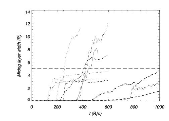
Figure 1: Evolution of the mean width of the jet/ambient mixing layer with time for all the simulations. Different types of lines are used for models with different internal energies: Continuous line: model A; dotted line: model B; dashed line: model C; dashed-dotted line: model D. Line thickness increases with Lorentz factor (from 5, thinest line, to 20 thickest one). A value of 5 $R_{\rm j}$ for the width of the mixing layer (horizontal dashed line) serves to classify the evolution of the different models.

3.1 Fully nonlinear evolution: jet/ambient mixing

The beginning of the mixing phase can be detected by the spreading of the tracer contours. This can be seen in Fig. 1, where the evolution with time of the mean width of the layer with tracer values between 0.05 and 0.95 is shown. The times at which the mixing phase starts ($t_{\rm mix}$) are shown in Table 2. Consistently with the width of the initial shear layer in our simulations (around 0.1 $R_{\rm j}$), we have defined $t_{\rm mix}$ as the time at which the mixing layer exceeds a width of 0.1 $R_{\rm j}$.

For models with the same thermodynamical properties, those with smaller Lorentz factors start to mix earlier (see Table 2). Moreover, according to Fig. 1, the models can be sampled in two (or perhaps three) categories. Models A05, B05, B10 and D10 have wide ($>5R_{\rm j}$) shear layers which are still in a process of widening at the end of the simulation. The rest of the models have thiner shear layers ($<5R_{\rm j}$ wide) which are inflating at smaller speeds ($0.5-2\,\,10^{-3}c$, in the case of models C05, D05 and C10; $0.5-1.2\,\,10^{-2}c$, in the case of models B20, C20, and D20). A deeper analysis of the process of widening of the shear layers as a function of time shows that all the models undergo a phase of exponential growth extending from $t_{\rm mix}$ to soon after $t_{\rm peak}$.

We note that those models developing wider mixing layers are those in which the peak in the maxima of the pressure perturbation as a function of time, $\Delta_{\rm peak}$, reach values of the order of $70-100$, with the exception of model B20 that has a thin mixing layer at the end of the simulation but has $\Delta_{\rm peak}\approx 100$, and model D10, which does develop a wide shear layer but for which $\Delta_{\rm peak}$ remains small. We also note that (with the exception of model D10) the models developing wide mixing layers are those with smaller internal energies and also relatively smaller Lorentz factors.

There are two basic mechanisms that contribute to the process of mixing between ambient and jet materials. The first one is the deformation of the jet surface by large amplitude waves during the saturation phase. This deformation favors the transfer of momentum from the jet to the ambient medium and, at the same time, the entrainment of ambient material in the jet. From Table 2, it is seen that the process of mixing and momentum exchange overlap during the saturation phase.

The second mechanism of mixing starts during the transition to the full non-linear regime and seems to act mainly in those models with large $\Delta_{\rm peak}$. As we shall see below, this large value of $\Delta_{\rm peak}$ is associated with the generation of a shock at the jet/ambient interface at $t_{\rm peak}$, which appears to be the responsible of the generation of wide mixing layers in those models. Figure 2 shows a sequence of models with the evolution of mixing in two characteristic cases, B05 and D05, during the late lapse of the saturation phase. The evolution of model B05 is representative of models A05, B05 and B10. Models B20, C05, C10, C20 and D10 have evolutions closer to model D05. As it is seen in Fig. 2, in the case of model B05 (left column panels), the ambient material carves its way through the jet difficulting the advance of the jet material which is suddenly stopped. The result is the break-up of the jet. In model D05, (right column panels), matter from the jet at the top of the jet crests is ablated by the ambient wind forming vortices of mixed material filling the valleys.

The large amplitude of $\Delta_{\rm peak}$ reached in models A05, B05 and B10 is clearly associated with a local effect occurring in the jet/ambient interface (see second panel in the left column of Fig. 2 and Fig. 3) that leads to the jet disruption. The sequence of events preceding the jet disruption includes the formation of oblique shocks at the end of the linear/saturation phase, the local effect in the jet/ambient interface just mentioned and then a supersonic transversal expansion of the jet that leads to i) a planar contact discontinuity (see last panels in the left column of Fig. 2), and ii) the formation of a shock (see below) that propagates traversally (see Sect. ss:transversal). It appears that contrary to the velocity perturbations in the jet reference frame (see Fig. 1 of Paper I), the maximum relative amplitudes of pressure perturbation are strongly dependent on physical parameters of simulations. The origin of the shock in models with $\Delta_{\rm peak}\approx 100$, that enhances the turbulent mixing of the jet and ambient fluids, can be found in the nonlinear evolution of Kelvin-Helmholtz instability that leads to significant changes of local flow parameters at the end of saturation phase. For instance, the oblique shock front resulting from the steepening of sound waves, during the linear and saturation phases (see Figs. 3-6 of Paper I), crosses the initial shear layer at the interface of jet and ambient medium. The formation of such oblique shock implies a sudden and local growth of gradients of all the dynamical quantities at the jet boundary. The local conditions changed by these oblique shocks may become favourable for the development of other instabilities like those discussed by Urpin (2002).

The generation of the shock wave at the jet/ambient interface is reflected in the evolution of the maxima of M${}_{j,\perp}=\gamma_{j,\perp}v_{j,\perp}/(\gamma_{c_{sa}}c_{sa})$ ($\gamma_{j,\perp}$ and $\gamma_{c_{sa}}$ being the Lorentz factors associated with $v_{j,\perp}$ and $c_{sa}$, respectively) representing the transversal Mach number of the jet with respect to the unperturbed ambient medium. This quantity becomes larger than 1 around $t_{\rm peak}$ in those models with $\Delta_{\rm peak}\approx 100$ (see Fig. 4) pointing toward a supersonic expansion of these jets at the end of the saturation phase. The fact that in all our simulations the ambient medium surrounding colder models (i.e., A, B) are also colder (see Sect. 2) favors the generation of shocks in the jet/ambient interface in these models. On the other hand, in the case of models with the highest Lorentz factors (B20, C20, D20) the transversal velocity can not grow far enough to generate the strong shock which breaks the slower jets.

 

 

 

 

 

 

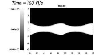
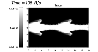
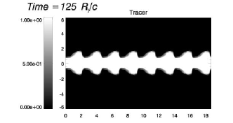
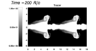
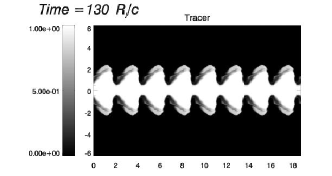
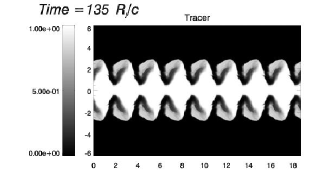
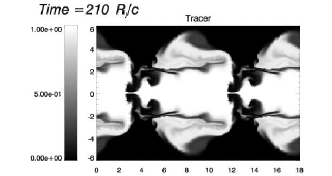
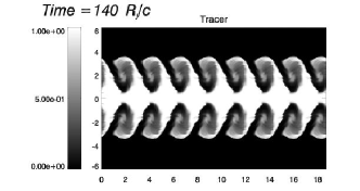
Figure 2: Evolution of the jet particle fraction showing the development of mixing in two representative models. Left column (model B05): the ambient material carves its way through the jet difficulting the advance of the jet material which is suddenly stopped. Right column (model D05): the amount of ambient matter hampering the jet material is smaller and matter from the jet at the top of the jet crests is ablated by the ambient wind.

 

 

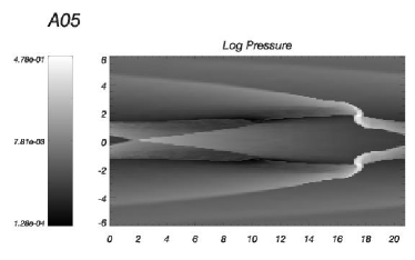
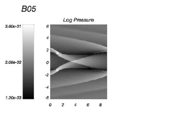
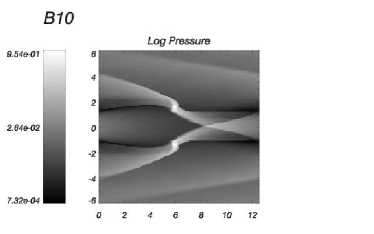
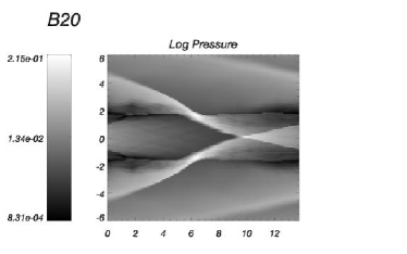
Figure 3: Pressure distribution at the onset of the jet/ambient surface distortion at the end of the saturation phase for models A05, B05, B10 and B20. The corresponding times are 355, 190, 370 and 765 $R_{j}/c$. In the case of models A05, B05 and B10 this distortion leads to the formation of a shock.

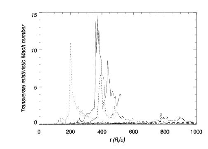
Figure 4: Time evolution of the maxima of the transversal Mach number of the jet with respect to the unperturbed ambient medium, M_j,⟂. See text for further explanations. Lines are as in Figure 1.

In order to extend our conclusions to a wider region in the initial parameter space, we have performed supplementary simulations (namely F, G, H, I, J, K, L) with the aim of clarifying the effect of the ambient medium in the development of the disruptive shock appearing after saturation. In all the cases, the external medium is that of model A05.

From models F to H, internal energy in the jet is increased and rest-mass density decreased in order to keep pressure equilibrium, whereas the jet Lorentz factor is kept constant to its value in model A05. The transversal Mach numbers at the peak in these models reach values very similar to that of model A05 ($\simeq 14$). In fact, the formation of a shock at the end of the saturation phase is observed in these models as it is in model A05.

The initial momentum density in the jet has decreased along the sequence A05, F, G, H. Simulations I and J have the same thermodynamical values as models F and G, respectively, but have increasing jet Lorentz factors to keep the same initial momentum density as model A05. In the case of model I we find the same behavior as in previous ones: large transversal Mach number, shock and disruption. On the contrary, model J behaves much more like model B20, with a value of transversal Mach number slightly larger than one, strong expansion and almost no mixing. Finally, in order to know to which extent this change in behavior was caused by the increase in Lorentz factor or in specific internal energy, in simulations K and L we cross these values with respect to those in I and J. The results from these last simulations show that the evolution of model M is very close to that of model I: the large value of the transversal Mach number at the peak, shock and strong mixing; and that the evolution of model K is close to that of model J: a weaker shock, expansion and no mixing.

In the models developing a shock, mixing is associated with vorticity generated after the shock formation and, in the case of models A05, B05, B10 as well as F, G, H, I and L matter from the ambient penetrates deep into the jet as to reach the jet axis (jet break-up). The times at which this happens for the different models are displayed in Table 2. Note that in models A05 and B05 the entrainment of ambient matter up to the axis occurs just after $t_{\rm peak}$, whereas in model B10 occurs later, probably because the shock in this model is weaker. The process of mixing can be affected by resolution, as small resolutions may suppress the development of turbulence. We have analyzed this in the Appendix in which we focus on the influence of longitudinal resolution.

3.2 Fully nonlinear evolution: jet/ambient momentum transfer

Let us now analyze the evolution of the longitudinal momentum in the jets as a function of time. Figure 5 shows the evolution of the total longitudinal momentum in the jet for the different models. Jets in models B05, C05, D05 and D10 (also D20) transfer more than 50% of their initial longitudinal momentum to the ambient, whereas models A05, B10 and C10 (also B20) seem to have stopped the process of momentum transfer retaining higher fractions of their respective initial momenta. Models C20 and D20 continue the process of momentum exchange at the end of the simulations but at a remarkable slower rate (specially C20).

In the case of models F, G, H, I and L, the transfer of longitudinal momentum is also very efficient. The reason why these models, as well as A05, B05 and B10, develop wide shear layers and transfer more than 50% of their initial momentum to the ambient could be turbulent mixing triggered by the shock. In the case of models D10 and D20, the processes of mixing and transfer of longitudinal momentum proceed at a slower rate pointing to another mechanism. The plots of the time evolution of the jet’s transversal momentum (Fig. 6) for the different models give us the answer. Jets disrupted by the shock (as A05, B05, B10) have large relative values of transversal momentum at saturation ($>0.04$) that decay very fast afterward (A05 is an exception). The peak in transversal momentum coincides with the shock formation and the fast lateral expansion of the jet at $t_{\rm peak}$. Contrarily, models D10 and D20 have a sustained value of transversal momentum after saturation which could drive the process of mixing and the transport of longitudinal momentum. In these models, the originally high internal energy in the jet and the high jet Lorentz factor (that allows for a steady conversion of jet kinetic energy into internal) make possible the sustained values of transversal momentum. Between these two kinds of behavior are hot, slow models C05, D05 that do not develop a shock having, then, thin mixing layers, but transferring more than 50% of their longitudinal momentum.

3.3 Fully nonlinear evolution: classification of the models

Our previous analysis based in the width of the mixing layers and the fraction of longitudinal momentum transfered to the ambient can be used to classify our models:

• Class I (A05, B05, B10, F, G, H, I, L): develop wide shear layers and break up as the result of turbulent mixing driven by a shock.

• Class II (D10, D20): develop wide shear layers and transfer more than 50% of the longitudinal momentum to the ambient, as a result of the sustained transversal momentum in the jet after saturation.

• Class III (C05, D05): have properties intermediate to models in classes I and II.

• Class IV (B20, C10, C20, J, K): are the most stable.

Figures 7-10 show the flow structure of the different models at the end of the simulations. The following morphological properties of the members of each class are remarkable:

• Class I: irregular turbulent pattern of the flow, the structure of KH modes still visible on the background of the highly evolved mean flow pattern.

• Class II: a regular pattern of ”young” vortices (visible in the tracer and specific internal energy distributions), the structure of KH modes visible. The enhanced transfer of momentum found in the models of this class is probably connected to the presence of these ”young” vortices.

• Class III: the flow is well mixed, i.e. tracer, internal energy and Lorentz factor are smoothed along lines parallel to the jet symmetry plane. Highly evolved vortices visible. A fossil of KH modes visible only as pressure waves.

• Class IV: no vortices, no chaotic turbulence, very weak mixing, very regular structure of KH modes.

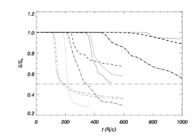
Figure 5: Evolution of the total longitudinal momentum in the jet as a function of time for all the simulations. Lines represent the same models than in Fig. 1. The long-dashed horizontal line serves us to identify those models tranferring more than 50% of the initial jet momentum to the ambient.

   

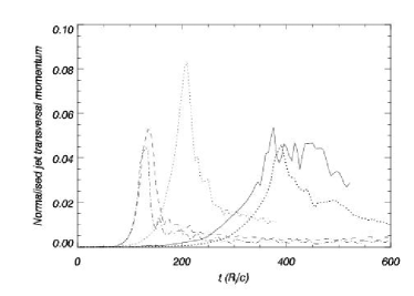
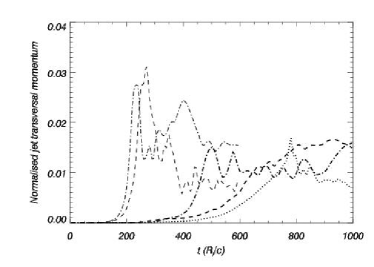
Figure 6: Evolution of the total transversal momentum in the jet as a function of time for all the simulations. Lines represent the same models than in Fig. 1. Left panel: models A05, B05, B10, C05, D05. Right panel: B20, C10, C20, D10, D20. Note the change in both horizontal and vertical scales between the two panels.

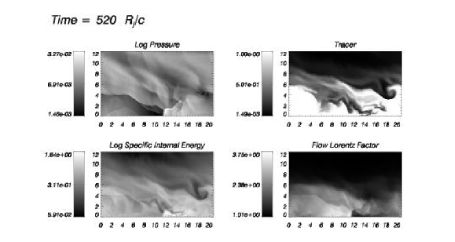
Figure 7: Snapshot in the mixing phase of logarithmic maps of pressure, jet mass fraction and specific internal energy and non-logarithmic Lorentz factor for model A05. Only the top half of the jet is shown.

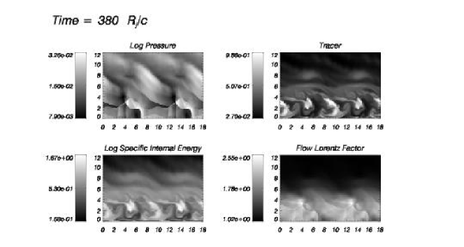
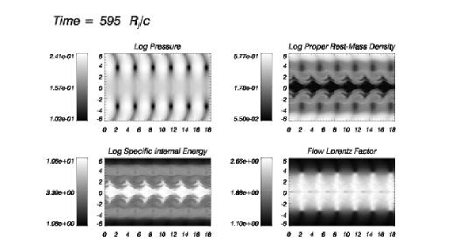
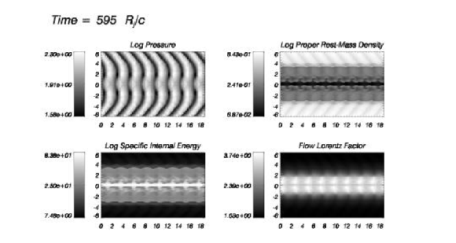
Figure 8: Same as Fig. (7) for models B05 (upper; only top half of the model shown), C05 (middle) and D05 (lower).

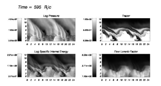
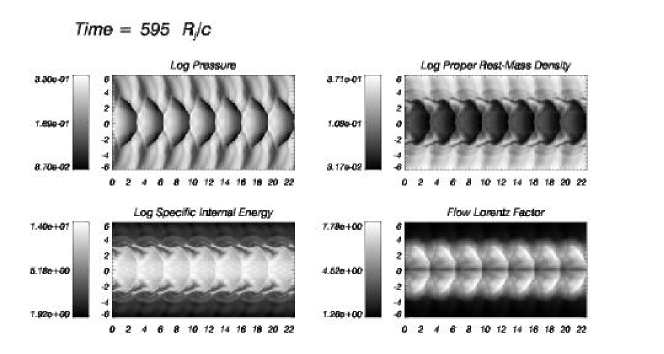
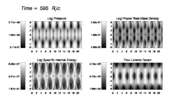
Figure 9: Same as Fig. (7) for models B10 (upper; only top half of the model shown), C10 (middle) and D10 (lower; only top half of the model shown).

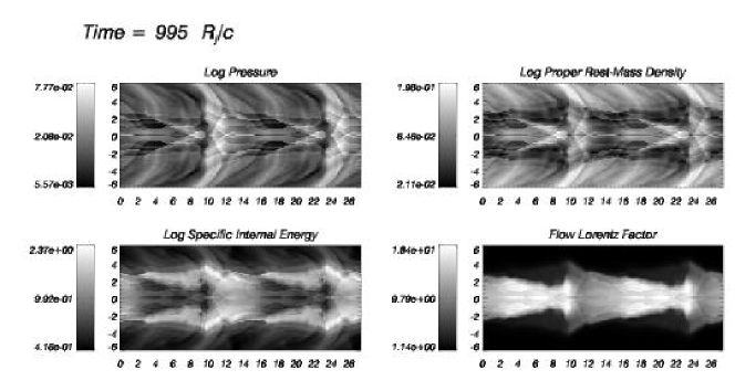
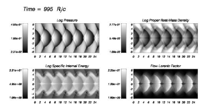
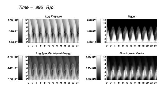
Figure 10: Same as Fig. (7) for models B20 (upper), C20 (middle) and D20 (lower; only top half of the model shown).

3.4 Transversal jet structure at late stages of evolution

At the end of our simulations, the models continue with the processes of mixing, transfer of momentum and conversion of kinetic to internal energy, however they seem to experience a kind of averaged quasisteady evolution which can be still associated with the evolution of a jet, i.e., a collimated flux of momentum. This jet is always wider, slower and colder than the original one and is surrounded by a broad shear layer. This Section is devoted to the examination of the transition layers in distributions of gas density, jet mass fraction and internal energy as well as shearing layers in velocity, longitudinal momentum and Lorentz factor.

Let us start by analyzing the overall structure of the pressure field for the different models at the end of our simulations. Figure 11 shows the transversal, averaged profiles of pressure accross the computational grid. Several comments are in order. In the case of models A and B, the shock formed at the end of the saturation phase is seen propagating (at $r\approx 30R_{j}$ in the case of model A, and at $r\approx 40-60R_{j}$ in the case of models B) pushed by the overpressure of the post shock state. In the case of models C and D, the wave associated with the peak in the pressure oscillation amplitude seem to have left the grid (remember that in our jet models, hotter jets have also hotter ambient media). The most remarkable feature in the pressure profile is the depression centered at $r\approx 2R_{j}$ in the case of models C10 and C20 and at $r\approx 3R_{j}$ in the case of models D10, D20. These pressure minima coincides with the presence of vortices (clearly seen in models C20 and D20 in the corresponding panels of Fig. 9 and Fig. 10). Also remarkable in these plots is the almost total pressure equilibrium reached by models C05 and D05 and the overpressure of the jet in model D20.

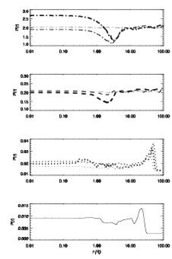
Figure 11: Longitudinal averaged profiles of gas pressure for all models. Different types of lines are used for models with different internal energies: Continuous line: model A; dotted line: model B; dashed line: model C; dashed-dotted line: model D. Line thickness increases with Lorentz factor (from 5, thinest line, to 20 thickest one).

As we noted in the previous Section the models evolve following four schemes. Jets belonging to the classes I and II disrupt leading to the dispersion of tracer contours for more than five initial jet radii. Model D20 of the II class is specific. It has not reached the tracer contour dispersion equal to five jet radii, but it clearly follows from Fig. 1 that this should happen around $t=1100$. The models belonging to the classes III and IV do not exhibit the dispersion of tracer contours for more than 5 jet radii and look different at the end of simulations.

Fig. 12 displays, for models B05 and D05 representing classes I/II and III/IV respectively, the profiles of relevant physical quantities averaged along the jet at the end of the simulations. Let us note that different shear (in case of velocity related quantities) or transition layers (in case of material quantities) can be defined depending on the physical variable used.

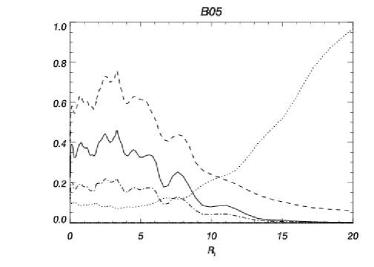
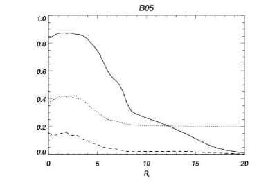
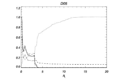
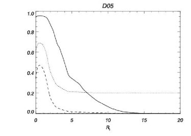
Figure 12: Transversal averaged profiles of relevant physical quantities at the end of simulations B05 and D05. Left column: tracer, $f$ (full line), rest mass density, $\rho_{0}$ (dotted line), specific internal energy $\varepsilon$ (dashed line) and jet internal energy density , $e$ ($=\rho_{0}\varepsilon f$; dash-dot line). Right column: longitudinal velocity, $v_{z}$ (full line), Lorentz factor normalized to its initial value, $\gamma/\gamma_{0}$ (doted line) and longitudinal momentum normalized to its initial value, $S/S_{0}$. The upper plots represent the model B05 and the lower plots represent D05. Note that the values of $e$ are multiple by 10 for model B05 and divided by 10 for model D05. The values of $\varepsilon$ for the model D05 are divided by 100.

In case of model B05 all the material quantities (tracer, density and internal energy) exhibit a wide broadening in the radial direction. The distribution of tracer extends up to $r=15R_{j}$, which means that jet material has been spread up to this radius, with a simultaneous entrainment of the ambient material into the jet interior. The latter effect is indicated by the lowering of the maximum tracer value from 1 down to 0.4. The fine structure of the tracer distribution displays random variations, which apparently correspond to the turbulent flow pattern well seen in Fig. 8 (upper set of panels). The curve of internal energy is very similar to the one corresponding to tracer, however variations are seen up to $r=20R_{j}$. The profile of density is wider than the profile of the tracer (the density is growing up to $r\sim 40R_{j}$, which can be explained by the heating of external medium, in the jet neighborhood, by shocks associated with outgoing large amplitude sound waves and by transversal momentum transmitted to the ambient medium via sound waves. Finally, the profile of the specific internal energy is consistent with the density profile and the fact of the jet being in almost pressure equilibrium.

The dash-dot curve in Fig. 12 (top left panel) represents the (internal) energy per unit volume held in jet matter. Such a quantitiy, like the mean Lorentz factors in both inner jet and shear layer are of special importance as they are directly related to the emission properties of the model. Internal energy density in jet particles is related to the fluid rest frame synchrotron emissivity, whereas the fluid Lorentz factor governs the Doppler boosting of the emitted radiation. As seen in the top right panel of Fig. 12, the final mean profile of velocity is similar in shape to the profile of internal energy, despite the fact that it is smoother. Similarly to internal energy, the longitudinal velocity variations extend up to $r=20R_{j}$. This can be understood in terms of large amplitude, nonlinear sound waves, which contribute to the transport of internal and kinetic energies in the direction perpendicular to the jet axis. The profiles of Lorentz factor and longitudinal momentum are significantly narrower. Therefore in case of models similar to B05 only the the most internal part, up to $r\leq 8R_{j}$ of the wide sheared jet, will be Doppler boosted, even though the jet material quantities extend behind $r\simeq 15R_{j}$.

A similar discussion can be performed for the model D05 representing the other group of jets, which form a shear layer without experiencing the phase of rapid disruption. As seen in the bottom panels of Fig. 12, the jet of model D05 preserves sharp boundaries between their interior and the ambient medium, although both media are modified by the dynamical evolution at earlier phases. The sharp boundary (transition layer) at $r\simeq 3.2R_{j}$ is apparent in the plots of all material quantities, i.e. tracer, density, internal energy. The thickness of the transition layer for all the quantities is comparable to one initial jet radius, 10 times narrower than in case of B05. We note, however a smooth change of ambient gas density in the range of $r\sim 3.2R_{j}\div 12R_{j}$.

It is apparent also that a narrow core of almost unmixed ($f=1$) jet material remains at the center in the currently discussed case. The radius of the core is about one half of the original jet radius. The core sticks out from a partially mixed, relatively uniform sheath and is well seen in the plots of tracer and internal energy for that model, however it disappears when increasing the resolution in the longitudinal direction, as seen in the Appendix.

Concerning the dynamical quantities, we note that there is no sharp jump in the profiles of longitudinal velocity, Lorentz factor and longitudinal momentum and the central core does not appear in profiles of these quantities. Significant longitudinal velocities extend up to $r\simeq 12R_{j}$ as in case of density, in contrast to tracer and internal energy. As noted previously, the averaged pressure distribution for model D05 is practically uniform in the whole presented range of the transversal coordinate. Therefore as in case B05 we can conclude that the variations of density in the ambient medium are due to the heat deposited by nonlinear sound waves. On the other hand the widths of the profiles of the Lorentz factor and longitudinal momentum are comparable to those of jet mass fraction and specific internal energy. Then the emission of the whole jet volume will be Doppler boosted.

Models B05 and D05 were considered as representative cases of models developing shear layers wider (group 1; classes I and II) and narrower (group 2; classes III and IV), respectively, than $5R_{j}$. Now the question is up to which extent the characteristics of the shearing flow of these two models are common to the models in the corresponding groups. We note that given the large differences between the initial parameters of models in classes I and II, on one hand, and III and IV, on the other, we do not expect a perfect match among the properties of the transversal structure in models within the same group. For example, whereas models in class I develop wide shear layers due to the action of a strong shock formed at the end of the saturation phase, models in class II develop shear layers through a continuous injection of transversal momentum and the generation of large vortices at the jet ambient interface.

We now investigate relations among the following averaged quantities in the whole set of models at the final state: the dispersion of tracer contours, the typical widths of profiles of density, internal energy density in jet matter ($r_{e}$), velocity, Lorentz factor ($r_{\gamma}$) and longitudinal momentum ($r_{S}$) and the peak values of Lorentz factor and the longitudinal momentum ($S_{\rm max}$). In all cases the peak values were measured directly, whereas the typical width of the profiles were taken as their width at the mean value between the maximum and minimum ones. We find that for all models of group 1, $r_{\gamma}>4R_{j}$, $r_{S}>3.5R_{j}$, $r_{e}>7R_{j}$ and $S/S_{0}<0.2$. In case of all models of group 2, $r_{\gamma}<4R_{j}$, $r_{S}<3.5R_{j}$, $r_{e}<7R_{j}$ and $S_{\rm max}/S_{0}>0.2$.

4 Discusion and conclusions

We have studied the non-linear evolution of the relativistic planar jet models considered in Paper I. The initial conditions considered cover three different values of the jet Lorentz factor (5, 10, 20) and a few different values of the jet specific internal energy (from 0.08$c^{2}$ to 60.0$c^{2}$). The models have been classified into four classes (I to IV) with regard to their evolution in the nonlinear phase, characterized by the process of mixing and momentum transfer. Cold, slow jets (Class I) develop a strong shock in the jet/ambient interface at the end of the saturation phase leading to the development of wide, mixed, shear layers. Hot fast models (Class II) develop wide shear layers formed by distinct vortices and transfer more than 50% of the longitudinal momentum to the ambient medium. In models within this class, the high Lorentz factor in the original jet and its high internal energy act as a source of transversal momentum that drives the process of mixing and momentum transfer. Between these classes we find hot, slow models (Class III) that have intermediate properties. Finally we have found warm and fast models (Class IV) as the most stable. Whether a jet is going to develop a strong shock and be suddenly disrupted seems to be encoded in the peak of the pressure oscillation amplitude at the end of the saturation phase and the related transversal Mach number.

The above picture is clarifying but is subject to the limitations of our choice of initial parameters that was restricted to values with $\rho_{\rm 0j}=0.1$ (see Paper I). This restriction together with the initial pressure equilibrium lead to a constant jet-to-ambient ratio of specific internal energies for all the models, i.e., hotter jets are surrounded by hotter ambient media. In order to extend our conclusions to a wider region in the initial parameter space, we have performed a supplementary set of simulations (F-L) with the aim of disentangling the effect of the ambient medium in the development of the disruptive shock appearing after saturation. Thus, hot, tenuous, slow/moderately fast jets (F, G, H, I, L) behave like cold, dense ones in a cold environment (A05, B05, B10). However, if these hot, tenuous jets are faster (J, K), they behave as warm, fast models (e.g., C10, C20, B20). The fact that the initial Lorentz factor is high seems to prevent the transversal velocity from growing enough to generate the strong shock which breaks the slower jets.

Models undergoing qualitatively different non-linear evolution are clearly grouped in well-separated regions in a jet Lorentz factor/jet-to-ambient enthalpy diagram (see Fig. 13). Models in the lower, left corner (low Lorentz factor and small enthalpy ratio) are those disrupted by a strong shock after saturation. Those models in the upper, left corner (small Lorentz factor and hot) represent a relatively stable region. Those in the upper right corner (large Lorentz factor and enthalpy ratio) are unstable although the process of mixing and momentum exchange proceeds on a longer time scale due to a steady conversion of kinetic to internal energy in the jet. Finally, those in the lower, right region (cold/warm, tenuous, fast) are stable in the nonlinear regime.

Our results differ from those of Martí et al. (1997), Hardee et al. (1998) and Rosen et al. (1999) who found fast, hot jets as the more stable. The explanation given by Hardee et al. (1998) invoking the lack of appropriate perturbations to couple to the unstable modes could be partially true as fast, hot jets do not generate overpressured cocoons that let the jet run directly into the nonlinear regime. However, as pointed out in Paper I, the high stability of hot jets may have been caused by the lack of radial resolution, that leads to a damping in the perturbation growth rates. Finally, the simulations performed in the aforementioned papers only covered about one hundred time units, well inside the linear regime of the corresponding models for small perturbations. In this paper, the problem of the stability of relativistic jets is analyzed on the basis of long-term simulations that extend over the fully nonlinear evolution of KH instabilities.

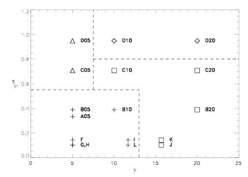
Figure 13: Square root of the jet-to-ambient enthalpy ratio (see Paper I for definitions) versus jet Lorentz factor. Symbols represent different non-linear behaviors: crosses stand for shock disrupted jets (cold, slow jets, along with tenuous, hot, moderately fast or slow ones); diamonds for unstable, hot, fast jets; triangles for relatively stable hot, slow, and squares for stable, warm, fast, along with hot, tenuous, faster jets.

At the end of our simulations, the models continue with the processes of mixing, transfer of momentum and conversion of kinetic to internal energy, however they seem to experience a kind of averaged quasisteady evolution which can be still associated with the evolution of a jet, i.e., a collimated flux of momentum. This jet is always wider, slower and colder than the original one and is surrounded by a distinct shear layer. Hence transversal jet structure naturally appears as a consequence of KH perturbation growth. The widths of these shear (in case of velocity related quantities) or transition layers (in case of material quantities) depend on the specific parameters of the original jet model as well as the physical variable considered. However, models in classes III and IV develop thin shear layers, whereas the shear layers of models in classes I and II are wider. The possible connection of these results to the origin of the FRI/FRII morphological dichotomy of jets in extended radiosources will be the subject of further research. Extensions of the present study to models with a superposition of perturbations, cylindrical symmetry and three dimensions are currently underway.

Appendix A Influence of numerical resolution in the nonlinear evolution

In order to be aware of the limitations of the resolution used in the results for the non-linear regime, we repeated model C05 (C16 here) with the same transversal resolution (400 cells/$R_{\rm j}$) and changing the longitudinal resolution. First we double it (32 cells$/R_{\rm j}$, C32) and then multiply it by four (64 cells$/R_{\rm j}$,C64), and finally, in order to have similar resolutions in both transversal and longitudinal directions, we performed this simulation using 256$\times$128 cells$/R_{\rm j}$ (C128). Models C16, C32 and C64 were evolved up to a time larger than 600 $R_{\rm j}/c$, whereas model C128 was stopped at $t=375R_{\rm j}/c$.

Table 3 displays the data corresponding to Table 2 for models C16, C32, C64, C128. Differences in the duration of the phases are apparent but not significant. Regarding the linear regime, perturbations in models C32 and C64 grow closer to linear predictions (growth rate 0.093 $c/R_{\rm j}$) in both cases; to be compared with the analytical value 0.114 $c/R_{\rm j}$) rather than C16 (0.085 $c/R_{\rm j}$). C128 has a slower growth rate (0.073 $c/R_{\rm j}$) due to its smaller transversal resolution (see Appendix of Paper I). Values of pressure perturbation at the peak range from 3 to 8, increasing generally from smaller to larger longitudinal resolution. Moreover, transversal relativistic Mach numbers are also increasing with resolution (from a value of about unity to two), so that we observe a stronger, although still weak, shock in C64 and C128 than in C16 or C32. This is maybe due either to the instability giving rise to the shock (see Section 3.1) being better captured with increasing resolution or as the result of a smaller numerical viscosity.

Figure 14 shows the time evolution of the mean width of the jet/ambient mixing layer and the total longitudinal momentum in the jet for model C05 as a function of resolution. No noticeable differences are found in the evolution of the different numerical simulations within the linear phase (up to $t\approx 100R_{\rm j}/c$). However, there is a clear tendency to develop wider mixing layers and enhance momentum transfer in those simulations with higher numerical resolutions as a result of the reduction of numerical viscosity. In the case of model C128 the processes of jet/ambient mixing and momentum exchange are further enhanced by the ratio of longitudinal to transversal resolution close to unity which favors the generation of vortices in the jet/ambient boundary. The enhancement of mixing with numerical resolution and the generation of vortices in model C128 is seen in the sequence of Panels for different simulations (see published paper) show that models C16 and C32 are very similar, whereas models C64 and C128 are totally mixed (see the maxima of the tracer values in the scales) and colder (as a result of the enhanced mixing with the cold ambient medium).

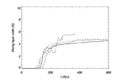
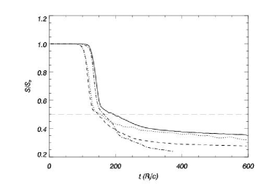
Figure 14: Same plots as 1 (left) and 5 (right) for models C16 (solid line), C32 (dotted line), C64 (dashed line) and C128 (dash-dotted line).

Finally, mean transversal profiles (appearing in the published paper) of relevant physical quantities show that the thin, hot core in model C16 disappears in model C128 due to the enhanced mixing. In model C32 mixing down to the axis occurs after a long process. Models C64 and C128 develop weak shocks after saturation and suffer sudden mixing, which goes on in time, cooling down the remaining relativistic flow. Transition layers in rest mass density, jet mass fraction and specific internal energy are wider in model C128 due to the enhanced mixing. Longitudinal velocity and momentum and Lorentz factor profiles are more similar in all the cases although the relativistic core is thinner in model C128.

$\begin{array}[]{cccccccc}\hline\cr{\rm Model}&t_{\rm lin}&t_{\rm mix}&t_{\rm sat}&t_{\rm peak}&\Delta_{\rm peak}&t_{\rm fmix}&t_{\rm meq}\\ \hline\cr{\rm C16}&100&120&125&130&5.0&>595&195\\ {\rm C32}&85&100&105&105&3.5&500&150\\ {\rm C64}&80&100&110&115&6.5&125&150\\ {\rm C128}&100&125&110&125&8.0&135&160\\ \hline\cr\end{array}$

Table 3: Times for different phases in the evolution of simulations C16, C32, C64 and C128. See Table 2 for the meaning of the times at the table entries.

References

- (1) Bodo, G., Massaglia, S., Ferrari, A., and Trussoni, E., Astron. Astrophys., 283, 655 (1994)
- Hanasz (1995) Hanasz, M., 1995, PhD Thesis, Nicholas Copernicus University, Toruń.
- Hanasz (1997) Hanasz, M., 1997, in Relativistic jets in AGNs, Ostrowski, M., Sikora, M., Madejski, G., Begelman, M., eds, Kraków, p. 85 (astro-ph 9711275)
- Hardee et al. (1998) Hardee, P.E., Rosen, A., Hughes, P.A., Duncan, G.C. 1998, ApJ, 500, 559
- (5) Martí, J.M, Müller, E., Font, J.A., Ibáñez, J.M, and Marquina, A., 1997, ApJ, 479, 151
- (6) Perucho, M., Hanasz, M., Martí, J.M, and Sol, H., 2004, A&A submitted
- Rosen et al. (1999) Rosen, A., Hughes, P.A., Duncan, G.C., Hardee, P.E. 1999, ApJ, 516, 729
- (8) Urpin, V. 2002, A&A, 385, 14