BA-TH/04-491

Bicocca-FT-04-9

astro-ph/0407573

Fitting Type Ia supernovae
with coupled dark energy

L. Amendola¹, M. Gasperini^2,3 and F. Piazza⁴

¹INAF/Osservatorio Astronomico di Roma,
Via Frascati 33, 00040 Monteporzio Catone (Roma), Italy

²Dipartimento di Fisica, Università di Bari,
Via G. Amendola 173, 70126 Bari, Italy

³Istituto Nazionale di Fisica Nucleare, Sezione di Bari, Italy

⁴Dipartimento di Fisica and INFN, Università di Milano Bicocca,
Piazza delle Scienze 3, I-20126 Milano, Italy

We discuss the possible consistency of the recently discovered Type Ia supernovae at $z>1$ with models in which dark energy is strongly coupled to a significant fraction of dark matter, and in which an (asymptotic) accelerated phase exists where dark matter and dark energy scale in the same way. Such a coupling has been suggested for a possible solution of the coincidence problem, and is also motivated by string cosmology models of “late time” dilaton interactions. Our analysis shows that, for coupled dark energy models, the recent data are still consistent with acceleration starting as early as at $z=3$ (to within 90% c.l.), although at the price of a large “non-universality” of the dark energy coupling to different matter fields. Also, as opposed to uncoupled models which seem to prefer a “phantom” dark energy, we find that a large amount of coupled dark matter is compatible with present data only if the dark energy field has a conventional equation of state $w>-1$.

There is increasing evidence that our Universe is presently in a state of cosmic acceleration [1] (or “late-time” inflation), i.e. that its energy is dominated by a component with negative (enough) pressure, dubbed “quintessence”, or dark energy. The energy density of such a cosmic component is, at present, comparable with that of the more conventional (pressureless) dark matter component, although their evolution equations can be widely different, in principle.

In order to alleviate such a “coincidence” problem [2], without fine-tuning and/or ad hoc assumptions on the viscosity of the dark matter fluid [3], a direct (and strong enough) coupling between dark matter (or at least a significant part of it) and dark energy has been proposed [4]. Phenomenological models of this type have been widely studied [4, 5, 6, 7], and shown to be compatible with various constraints following from supernovae observations, cosmological perturbation theory and structure formation. They are also theoretically motivated by the identification of the dark energy field with the string-theory dilaton [8, 9], and by the assumption that dilaton loop corrections saturate in the strong coupling regime [10].

A key feature of the coupled dark energy scenario is that it may allow a late-time attractor describing an accelerated phase, characterized by a frozen ratio $\rho_{\rm{dark~{}matter}}/\rho_{\rm{dark~{}energy}}$. This occurs, in models where a rolling scalar field $\phi$ plays the role of the cosmic dark energy, when the dark energy has an exponential potential and is exponentially coupled to scalar dark-matter fields (such an attractor property is lost, however, in the case of Yukawa-type interactions to fermionic dark matter [11]). For a successful scenario it is also required that $a)$ the present coupling of the scalar to some exotic dark matter component is strong enough and approximately constant, and $b)$ the present coupling to ordinary (baryonic) matter is weak enough, in order to avoid testable violations of the equivalence principle.

In addition, the cosmic dark energy field has to be either massless or ultra-light, with a mass $m\sim H_{0}$, where $H_{0}\simeq 10^{-33}$ eV is the present Hubble scale. For a scalar field gravitationally coupled to particles of mass $M$, on the other hand, there are quantum (radiative) corrections to the mass [12] of order $m\sim qM(\Lambda/M_{\rm P})$, where $q$ is the dimensionless coupling strength and $\Lambda/M_{\rm P}$ is the cut-off scale (typically, $1$ TeV), in Planck units. This well known perturbative argument seems to suggest that both the coupling $q$ to ordinary baryonic matter (for which $M\sim 1$ Gev), and the value of $M$ for the coupled, exotic dark matter components (for which the models assumes $q\simeq 1$), need to be fine-tuned at extremely low values [13]. It should be stressed, however, that scalars with masses comparable to the (four dimensional) curvature of the Universe could be safe from radiative corrections, thanks to a recently proposed mechanism based on the AdS/CFT correspondence [14].

Quite independently from theoretical motivations, and from possible interpretations in a string cosmology context, in this work we consider the basic scenario [4] in which dark energy is parametrized by a (canonically normalized) scalar field $\phi$, with exponential self-interaction energy of slope $\mu\sqrt{2/3}$,

$$V(\phi)=V_{0}e^{-\mu\sqrt{\frac{2}{3}}{\frac{\phi}{M_{\rm P}}}}.$$ (1)

Here $\mu>0$ and $M_{\rm P}=(8\pi G)^{-1/2}$ is the reduced Planck mass. Neglecting radiation, as we are concerned with the late evolutionary phase of our Universe, we can describe the remaining gravitational sources as a cosmic fluid of non-relativistic, “dust” particles, distinguishing however a “coupled” and “uncoupled” component, with energy densities $\rho{{}_{c}}$ and $\rho{{}_{u}}$, respectively. Uncoupled matter (for instance, baryons) satisfies the usual conservation equation

$$\dot{\rho{{}_{u}}}+3H\rho{{}_{u}}=0,$$ (2)

while the coupled evolution of $\rho{{}_{c}}$ and $\phi$ is described by the system of equations

$$\dot{\rho{{}_{c}}}+3H\rho{{}_{c}}-\beta{\sqrt{\frac{2}{3}}}{\frac{\dot{\phi}}{M_{\rm P}}}\rho{{}_{c}}=0,$$ (3)

$$\ddot{\phi}+3H\dot{\phi}+{\frac{\partial V}{\partial\phi}}+\beta{\sqrt{\frac{2}{3}}}{\frac{1}{M_{\rm P}}}\rho{{}_{c}}=0,$$ (4)

with $\beta{>}0$. The total energy density is finally normalized according to the Einstein equation

$$3M_{\rm P}^{2}H^{2}=\rho_{\phi}+\rho_{c}+\rho_{u},$$ (5)

where $\rho{{}_{\phi}}={\dot{\phi}^{2}/2}+V(\phi).$ To make contact with previous work, we have used the notations of [4, 5], but we stress that the above equations also describe the asymptotic “freezing” phase of a “running dilaton” model [8], provided we identify the slope $\mu\sqrt{2/3}$ and the coupling parameter $\beta{\sqrt{2/3}}$ of the present model with the slope $\lambda$ and the dilaton charge $q$ of [8] as follows:

$$\mu\sqrt{\frac{2}{3}}=\lambda,~{}~{}~{}~{}~{}~{}~{}\beta{\sqrt{\frac{2}{3}}}={\frac{q\lambda}{2}}.$$ (6)

The above equations can be derived (for a conformally flat metric) from the (Einstein-frame) action

$${S}\,\,=\,\,\int d^{4}x\sqrt{-g}\left[-\frac{M_{P}^{2}}{2}\,R+\frac{1}{2}(\nabla\phi)^{2}-V(\phi)\right]+{\mathcal{S}}_{c}[\phi,\psi_{c},g_{\mu\nu}]\,+{\mathcal{S}}_{u}[\psi_{u},g_{\mu\nu}],$$ (7)

where $\psi_{c}$ and $\psi_{u}$ are the coupled and uncoupled matter fields, respectively. The parameter $\beta{}$ is thus related to the (homogeneous) scalar charge density, $\delta S_{c}/\delta\phi$, of coupled matter, as

$$\beta{\sqrt{\frac{2}{3}}}=-{\frac{M_{\rm P}}{\rho{{}_{c}}\sqrt{-g}}}{\frac{\delta S_{c}}{\delta\phi}}.$$ (8)

As shown in [4, 8], such a system of equations is characterized by an asymptotic accelerated regime in which the uncoupled component has redshifted away, $\rho{{}_{u}}=0$, and all other terms of the Einstein equations have the same scaling behaviour:

$$V\propto\dot{\phi}^{2}\propto\rho{{}_{\phi}}\propto\rho{{}_{c}}\propto H^{2}\propto a^{-3(1+w)},~{}~{}~{}~{}\qquad w=-\frac{\beta}{\beta+\mu}$$ (9)

(a wider class of scalar field Lagrangians leading to similar attractor configurations has been studied in [9]). Within this regime $\rho{{}_{\phi}}/\rho{{}_{c}}=$ const, and $\Omega_{\phi}=\rho{{}_{\phi}}/3M_{\rm P}^{2}H^{2}$, $\Omega_{c}=\rho{{}_{c}}/3M_{\rm P}^{2}H^{2}$, are also constant. The evolution is accelerated, with constant acceleration parameter,

$${\frac{\ddot{a}}{aH^{2}}}=1+{\frac{\dot{H}}{H}}={\frac{q-1}{q+2}}={\frac{2\beta{-}\mu}{2\beta{+}\mu}},$$ (10)

provided $2\beta{>}\mu$ (or $q>1$ in the notations of [8]). The luminosity-distance relation, for this regime, is obtained from the Hubble function

$$H(z)=H_{0}(1+z)^{3(1+w)/2}$$ (11)

(see Eq. (9)), where $z(t)=a_{0}/a(t)-1$ is the red-shift parameter. The corresponding Hubble diagram is thus completely controlled by the dark energy parameter $w$, and its compatibility with previously known Type Ia supernovae (SNe Ia) has been studied in [5].

Motivated by the recent important discovery of many new SNe Ia at $z>1$ [15], the aim of this paper is to re-discuss a possible fitting of present supernovae data in the context of the above model of coupled dark energy. Instead of assuming the asymptotic regime as an appropriate description of our present cosmological state, here we consider a “quasi-asymptotic” configuration, describing a cosmological state in the vicinity of the attractor, and for which the uncoupled component $\rho{{}_{u}}$ is small, but nonzero. The function $H(z)$, and the associated luminosity-distance relation, will then be obtained by perturbing the “freezing” [8] (or “stationary” [4]) configuration (9), to the linear order. Such a perturbed configuration will contain the (critical) fraction of uncoupled matter, $\Omega_{u}$, as a parameter measuring the typical (phase-space) “distance” from the asymptotic attractor with $\Omega_{u}=0$ (a different model with coupled and uncoupled fraction of dark matter components has been recently considered also in [7]).

The uncoupled matter density scales in time faster than $\rho{{}_{c}}$, namely $\rho{{}_{u}}\sim a^{-3}\sim(1+z)^{3}$, exactly like the standard dark matter component. Unlike in conventional models of uncoupled quintessence, however, the fraction $\Omega_{u}$ of uncoupled matter is not to be identified with the total present fraction of non-relativistic (baryon+dark matter) components, and is not necessarily close to $0.3$. In the case discussed here, the present value of $\Omega_{u}$ may range from the minimum $\Omega_{u}=\Omega_{\rm{baryons}}\simeq 0.05$ (we will refer to this as the “minimal model”), to a maximum amount consistent with the clustered fraction of dust energy density $\Omega_{m}$. As a reference value, we will assume $\Omega_{m}=0.3$.

Such a different interpretation of $\Omega_{u}$, as we shall see, has two important consequences. The first one, already stressed in [5], is that the accelerated regime may have a longer past extension, starting at early epochs characterized by $z>1$, which are instead forbidden for the standard (i.e. uncoupled) quintessential models [15].

The second one, which probably represents the main result of this paper, is that a small enough value of $\Omega_{u}$ is consistent with present data only for $w>-1$. If we take, for instance, $\Omega_{u}<0.2$, we obtain $w>-1$ at the $99\%$ confidence level. More conventional analyses, assuming a fraction of uncoupled dark matter near to or larger than $\Omega_{m}\simeq 0.3$, seem to favour instead $w<-1$ [16], although $w>-1$ is certainly still consistent with data. Should future data confirm these results, we would be left with the choice between “phantom” models of dark energy [17], uncoupled to dark matter but plagued by severe quantum instabilities [18] (see, however, [19]), and dilaton-like models of dark energy [4]-[9], non-minimally coupled to a significant fraction of dark matter.

In order to perturb the dynamical system of coupled equations (2)-(5) it proves convenient to introduce the dimensionless variables

$$x^{2}=\frac{\dot{\phi}^{2}}{6M_{\rm P}^{2}H^{2}}\,,\qquad y^{2}=\frac{V}{3M_{\rm P}^{2}H^{2}}\,,\qquad u^{2}=\frac{\rho_{u}}{3M_{\rm P}^{2}H^{2}}\,.$$ (12)

Obviusly, $\Omega_{c}=1-x^{2}-y^{2}-u^{2}$. Denoting with a prime the derivative with respect to the evolution parameter $N=\ln(a/a_{0})$, the coupled system of equations, for the model presented in the previous section, can then be rewritten as [4, 20]:

$$x^{\prime} = -\frac{3}{2}\left(1-x^{2}+y^{2}\right)x-\mu y^{2}+\beta(1-x^{2}-y^{2}-u^{2}),$$

$$y^{\prime} = \mu xy+\frac{3}{2}y\left(1+x^{2}-y^{2}\right),$$

$$u^{\prime} = \frac{3}{2}u\left(x^{2}-y^{2}\right).$$ (13)

Since there is complete symmetry with respect to simultaneous sign inversion of $\beta,\mu$ and $\phi$, we will consider the case $\mu>0$ only. It is also useful to write the equation for the derivative of $H$: one has, from Eq. (5),

$$\frac{H^{\prime}}{H}=-\frac{1}{2}(3+3x^{2}-3y^{2}).$$ (14)

By equating the right hand sides of (13) to zero one obtains a system of algebraic equations whose solutions are characterized by constant fractional densities. Of particular interest is the freezing (or stationary) configuration, given by

$$x_{0}=-\frac{3}{2(\beta+\mu)}\,,\qquad y_{0}=\frac{\sqrt{9+4\beta\mu+4\beta^{2}}}{2(\beta+\mu)}\,,\qquad u_{0}=0.$$ (15)

This point exists for $\beta>0$ and $\mu>(-\beta+\sqrt{18+\beta^{2}})/2$, is accelerated for $\mu<2\beta$, and is a global attractor [4]. On this solution, the properties (9)-(11) are valid.

The energy budget of our present Universe includes however an uncoupled component of non-relativistic matter at least as abundant as baryons, namely $u^{2}\neq 0$, $u^{2}~{}\raise 1.72218pt\hbox{$>$}\kern-6.99997pt\lower 2.6694pt\hbox{$\sim$}~{}0.05$, which measures our “distance” from the solution (15). In order to study the transient phase of approach to the attractor we will assume that $u^{2}$ is small enough to be compatible with a perturbative approximation, and we linearize (13) around (15), obtaining

$$\delta x^{\prime} = (9x_{0}^{2}-3y_{0}^{2}-4\beta x_{0}-3)\frac{\delta x}{2}-[3x_{0}y_{0}+2y_{0}(\mu+\beta)]\delta y-\beta u^{2},$$

$$\delta y^{\prime} = (\mu y_{0}+3x_{0}y_{0})\delta x+(3x_{0}^{2}-9y_{0}^{2}+2\mu x_{0}+3)\frac{\delta y}{2}.$$ (16)

In this approximation, we will assume that $u^{2}$ scales in time following the asymptotic behaviour (9), namely

$$u^{2}=\Omega_{u}\left(a/a_{0}\right)^{3w}=\Omega_{u}e^{3wN}.$$ (17)

We may thus regard $u^{2}$ as a first-order “external source”, reducing (16) to an inhomogeneous system. The general solution is given by

$$\delta x = c_{11}e^{\varepsilon_{1}N}+c_{12}e^{\varepsilon_{2}N}+A_{1}u^{2}\,,$$

$$\delta y = c_{21}e^{\varepsilon_{1}N}+c_{22}e^{\varepsilon_{2}N}+A_{2}u^{2}\,.$$ (18)

The coefficients $c_{ij}$ characterize the solution of the homogeneous system with $u^{2}=0$. Their values depend on the initial conditions, while the exponents $\varepsilon_{1}$ and $\varepsilon_{1}$ are found by direct substitution to be

$$\varepsilon_{1}=-\frac{6\beta^{2}+9\beta\mu+3\mu^{2}{}}{4(\beta+\mu)^{2}}-\frac{\sqrt{D}}{4(\beta+\mu)}\,,\qquad\varepsilon_{2}=-\frac{6\beta^{2}+9\beta\mu+3\mu^{2}{}}{4(\beta+\mu)^{2}}+\frac{\sqrt{D}}{4(\beta+\mu)}\,.$$ (19)

The square root of

$$D=324-32\beta^{3}\mu-63\mu^{2}-4\beta\mu(8\mu^{2}-27)-4\beta^{2}(16\mu^{2}-45)$$ (20)

is always imaginary in the region $2\beta>\mu$, for which acceleration occurs. Therefore, the “homogeneous part” of (18) describes at the linear level the oscillatory behavior of the system while converging to the attractor. Such oscillations clearly appear also at the level of exact numerical solutions of the coupled equations, see for instance [4, 8]. However, the amplitudes $c_{ij}$ are always subdominat with respect to the inhomogeneous terms of Eq. (18), as shown by direct numerical integration of the linear system (16).

In describing the approach to the attractor the most relevant role is thus played by the inhomogeneous contributions, proportional to $u^{2}$. The coefficients $A_{1}$ and $A_{2}$ of Eq. (18) do not depend on the initial conditions, and are found to be

$$A_{1} = -\frac{27\beta}{8\beta\mu^{3}+2(9+8\beta^{2})\mu^{2}+4\beta\mu(2\beta^{2}-9)-9(9+4\beta^{2})},$$

$$A_{2} = -\frac{\beta[2\mu(\beta+\mu)-9]\sqrt{9+4\beta(\beta+\mu)}}{8\beta\mu^{3}+2(9+8\beta^{2})\mu^{2}+4\beta\mu(2\beta^{2}-9)-9(9+4\beta^{2})}.$$ (21)

By setting $c_{ij}=0$ we can then compute, from Eq. (14), the Hubble parameter, and we obtain, to first order,

$$2\frac{H^{\prime}}{H}=-3(1+w)-6\Omega_{u}(x_{0}A_{1}-y_{0}A_{2})e^{3wN}.$$ (22)

Direct integration leads then to the following approximate result for the perturbed Hubble parameter:

$$H^{2}=H_{0}^{2}\,\,e^{2\int_{0}^{N}dNH^{\prime}/H}= H_{0}^{2}e^{-3(1+w)N}\left[1-6\Omega_{u}(x_{0}A_{1}-y_{0}A_{2})\int_{0}^{N}dNe^{3wN}\right]$$

$$= H_{0}^{2}\left[(1-\Omega_{R})a^{-3(1+w)}+\Omega_{R}a^{-3}\right],$$ (23)

where we have introduce the “renormalized” fractional density of the uncoupled component, $\Omega_{R}$, defined by

$$\Omega_{R}=\Omega_{u}(1+\epsilon),~{}~{}~{}~{}~{}~{}~{}~{}~{}\epsilon\,\,=\,\,6\frac{y_{0}A_{2}-x_{0}A_{1}}{3w}-1\,\,=\,\,$$

$$=\frac{9(9+2\beta\mu)}{2\mu^{2}(9+8\beta^{2})+4\beta\mu(2\beta^{2}-9)-9(9+4\beta^{2})+8\beta\mu^{3}}.$$ (24)

Note that $\Omega_{R}/\Omega_{u}$ is always larger than (but near to) unity, for realistic values of $\beta{,}\mu$ [4]. In Fig. 1 we compare the result (23) for $H^{2}$ with a numerical integration of the exact equations (13) which includes the homogeneous part of the solution: the errors turn out to be very small, less than 3% in the range $z<6$.

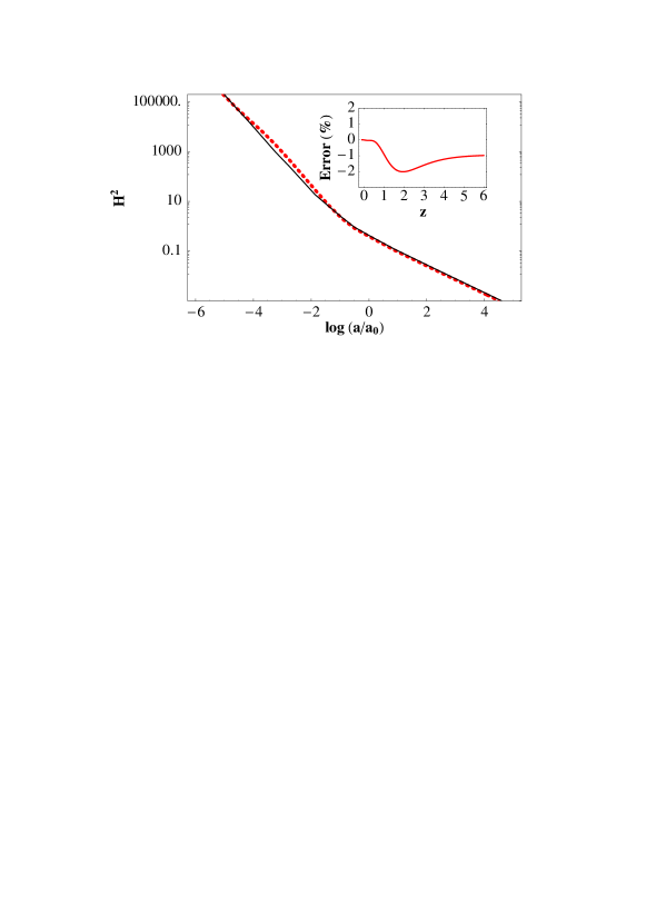
Figure 1: Approximations to $H^{2}$ (assuming $\beta=4,\mu=3,\Omega_{b}=0.05,\Omega_{c}=0.3$). The dotted curve is the numerical result, the full curve the linear fit. In the inset, the relative error.

The recent compilation of SNe Ia data can now be used to put constraints on the two parameters $\Omega_{R}$ and $w$ entering the expression for $H(a)$ in Eq. (23). Such an expression is formally identical to that of a conventional, perfect fluid model with a pressureless component, $\Omega_{R}$, and a dark energy component, $1-\Omega_{R}$, with constant equation of state. We have performed a numerical analysis with the gold sample of data presented in [15], and we have reproduced the same results as in [15] for constant equation of state, but we now interpret $\Omega_{R}$ as the total fraction of uncoupled matter rescaled by the (model-dependent) factor $1+\epsilon$.

In coupled dark energy models, characterized by Eq. (9), the effective equation of state of the asymptotic regime always corresponds to a parameter $w>-1$. We thus begin the analysis by restricting ourselves to this region of parameter space. We also notice that, in all subsequent plots, the likelihood function has been integrated over a constant offset of the apparent magnitude that takes into account the uncertainty on the absolute calibration both of the SN magnitude and of the Hubble constant. All results are therefore independent of the present value of the Hubble parameter.

In Fig. 2 we show the likelihood contours in the plane $(w,\Omega_{R})$. The value $\Omega_{R}\simeq\Omega_{u}=0.05$ lies near the limit of, but inside, the contour corresponding to the 90% confidence level. This shows that an uncoupled percentage of dark matter density of the order of the baryon density is not ruled out by present SNe Ia data. Moreover, if some fraction of dark matter is also actually uncoupled, the fit is generally improved. However, $\Omega_{u}$ cannot be arbitrarily close to $\Omega_{m}$, where $\Omega_{m}=\Omega_{u}+\Omega_{c}\simeq 0.3$ is the total non relativistic matter density that can be estimated through the mass in galaxy clusters. Moving toward the higher confidence regions of Fig. 2 requires indeed a lower and lower fraction of coupled dark matter, but the latter must be compensated with higher and higher values of the coupling $\beta$ in order to get an equivalent amount of acceleration.

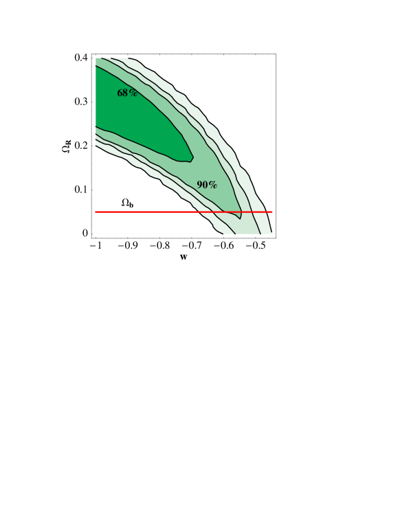
Figure 2: Contour plot obtained from the SNe Ia of [15], cutting to $w>-1$. Likelihood contours, from inside to ouside, are at the 68%, 90%, 95%, 99% confidence level. $\Omega_{R}$ is the effective fraction of uncoupled matter evolving as $a^{-3}$ (see Eq. (23)). The line labelled by $\Omega_{b}$ marks the present baryon fraction.

This point is better illustrated in Fig. 3, where the confidence regions are plotted in the $\beta$–$\Omega_{u}$ plane for $\Omega_{m}=0.27$. For a given value of the external parameter $\Omega_{m}$, in fact, any point of the $w-\Omega_{R}$ plane can be related to a point of the $\beta-\Omega_{u}$ plane, using Eq. (24) and the relation

$$\mu(\beta,\Omega_{m})=\frac{2\beta\Omega_{m}-\beta+\sqrt{\beta^{2}+18(1-\Omega_{m})}}{2(1-\Omega_{m})},$$ (25)

derived from $\Omega_{m}=1-x_{0}^{2}-y_{0}^{2}$, and valid near the attractor (we took the root that gives positive acceleration) . Values of $\Omega_{m}$ different from, but near to, 0.27, lead qualitatively to the same result.

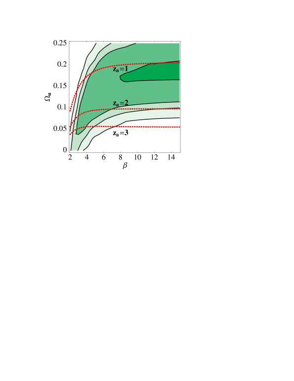
Figure 3: The SNe Ia results projected on the plane $\beta,\Omega_{u}$, at fixed $\Omega_{m}=0.27$. Likelihood contours, from inside to outside, are at the 68%, 90%, 95%, 99% confidence level. The dotted curves mark the parameter values for which $z_{\rm{acc}}$ equals $1$, $2$ and $3$, respectively. Values of $z_{\rm{acc}}$ above $1$ are within one $\sigma$, and even $z_{\rm{acc}}=3$ is not excluded at more than 90% c.l..

We can see from Fig. 3, where $\Omega_{m}$ has been fixed at a reasonable value, that we cannot arbitrarily shrink to zero the value of $\Omega_{c}$ without increasing $\beta$. A coupling $\beta$ much greater than unity, on the other hand, leads strong effective violations of the gravitational universality in the dark matter “subsector” corresponding to $\Omega_{c}$. Such violations are in principle constrained by present observations comparing the distribution of dark matter and baryons in galaxies and clusters [21]. The corresponding upper bounds derived on $\beta$, however, depend on several assumptions concerning the dark matter distribution and are of limited generality. Moreover, the bounds in [21] are derived assuming that all the dark matter is coupled, while here we are taking the more general point of view that $\Omega_{c}$ may differ from $\Omega_{m}$.

For all these reasons, a firm quantitative limit on $\beta$ is hard to be derived from present data, and will be discussed in a forthcoming paper [22]. In this paper we will not exclude a priori large values of $\beta$, taking into account, however, that the large couplings required for a good fitting to SN data could impose severe constraints on coupled models of dark energy.

In Fig. 3 we have also plotted the curves $z_{\rm{acc}}$ marking the beginning of the accelerated regime, which are obtained from Eq. (23) as

$$z_{\rm{acc}}(\Omega_{R},w)=[(3w+1)(\Omega_{R}-1)/\Omega_{R}]^{-1/3w}-1.$$ (26)

It follows that even $z_{\rm{acc}}=3$ cannot be excluded at more than 90% confidence level, while a value of $z_{\rm{acc}}>1$ is well within the 68% confidence level. This shows that the claim of [15] (see, however, [23]) about experimental detection of deceleration at $z>0.5$ does not apply to models of coupled dark energy.

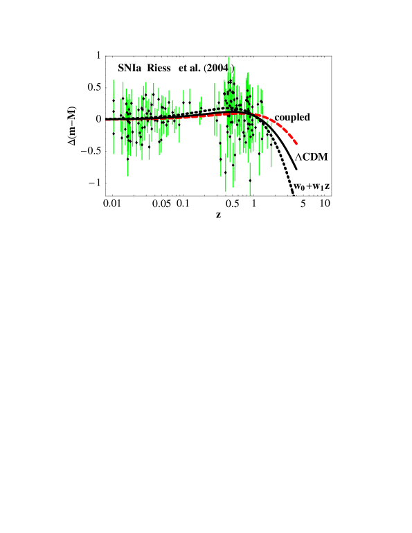
Figure 4: Best fits of the distance modulus $\Delta(m-M)$ for three different models: $\Lambda$CDM ($\Omega_{m}=0.27,\Omega_{\Lambda}=0.73$), coupled dark energy $(w=-0.6,~{}$$\Omega_{R}=0.05$ ) and a varying equation of state $w=w_{0}+w_{1}z$, with $w_{0}=-1.31$, $w_{1}=-1.48$, fixing $\Omega_{m}=0.27$. The data represent the gold sample of [15].

On a more qualitative level, we show in Fig. 4 the best fit of SNe Ia for three classes of models, compared to the dataset of [15]: the standard $\Lambda$CDM scenario, a varying equation of state with $w=w_{0}+w_{1}z$, and our coupled model. The plotted variable is the distance modulus $\Delta(m-M)\equiv(m-M)_{\rm{model}}-(m-M)_{\rm{Milne}}$, as customary (see for instance [24]), where apparent and absolute magnitude are related by

$$m-M=5\log_{10}d_{L}(z),~{}~{}~{}~{}~{}~{}~{}~{}~{}d_{L}(z)=(1+z)\int_{0}^{z}dz^{\prime}H^{-1}(z^{\prime}).$$ (27)

As it can be seen, the coupled model is almost degenerate (difference less than $\Delta m=0.1)$ with $\Lambda$CDM up to $z\approx 1.5$, and with the varying-$w$ model up to $z\approx 1$. However, in these three models, the acceleration begins at very different epochs ($z_{acc}=0.75$ for $\Lambda$CDM, $z_{acc}=0.69$ for $w=w_{0}+w_{1}z$, to be compared to $z_{acc}=3.53$ for the coupled model).

We can also perform the fit by including the region of parameter space with $w<-1$. In that case, the best fit moves to larger values of $\Omega_{u}$ (see Fig. 5). As a consequence, the baryon value $\Omega_{R}\simeq\Omega_{b}\simeq 0.05$ moves near the 97% confidence level. This shows, on one hand, that additional SNe Ia data may have the potential to disprove models in which all (or most of) dark matter is coupled to dark energy. On the other hand, this also shows that if the uncoupled fraction of dark matter is small enough, namely $\Omega_{u}~{}\raise 1.72218pt\hbox{$<$}\kern-8.00003pt\lower 2.6694pt\hbox{$\sim$}~{}\Omega_{R}~{}\raise 1.72218pt\hbox{$<$}\kern-8.00003pt\lower 2.6694pt\hbox{$\sim$}~{}0.2$, then we are lead to the region of parameter space with $w>-1$, excluding “phantom” or “k-essence” models of dark energy [17], possibly associated to embarrassing cosmic violations of the null energy condition.

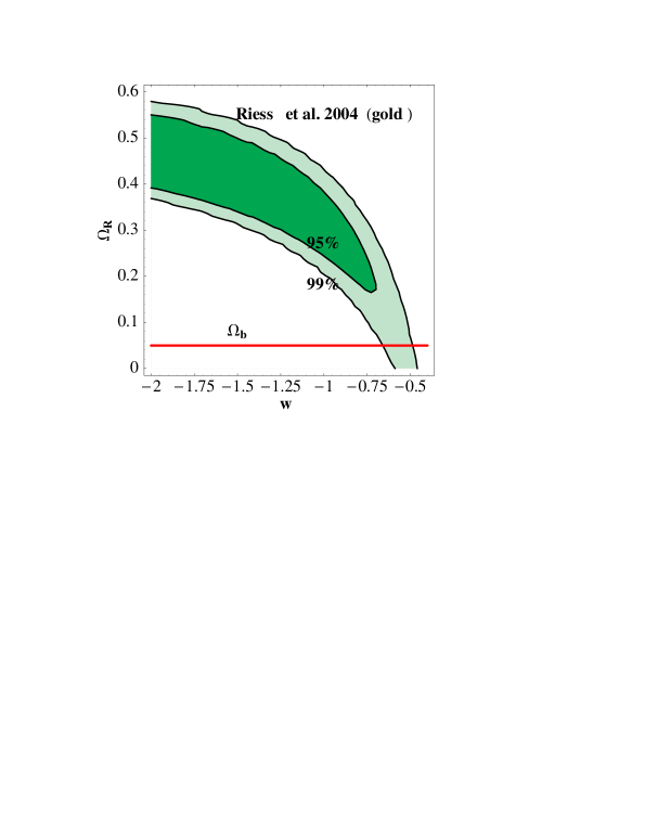
Figure 5: Contour plot obtained from the SNe Ia of [15], including $w<-1$. Likelihood contours, from inside to ouside, are at the 95% and 99% confidence level. The variables $w,\Omega_{R},\Omega_{b}$ are the same as in Fig. 2.

Finally, we can also derive constraints on $w$ alone by marginalizing over $\Omega_{R}$ (i.e. integrating the full likelihood over the domain of $\Omega_{R}$, see Fig. 6). In the minimal case in which the totality of (renormalized) uncoupled matter coincides with the baryon fraction, $\Omega_{b}$, we marginalize over $\Omega_{R}=0.05\pm 0.01$ (we disregard here the possible small difference between $\Omega_{u}$ and $\Omega_{R}$). The best fit turns out to be $w=-0.6\pm 0.05$, rather independently of the exact value of $\Omega_{R}$. If we keep instead the range $\Omega_{R}=0.04-0.3$, i.e. the full possible range of the uncoupled matter fraction, we then obtain $w=-0.8\pm 0.1$. This shows that, with some finite fraction of coupled matter, the allowed range of values of $w$ remains firmly anchored to the $w>-1$ region of parameter space, in contrast with the standard case in which $\Omega_{R}\approx 0.3\pm 0.05$, for which the peak of the likelihood is at $w\approx-1.1$ and the likelihood content of the $w<-1$ region is 80%.

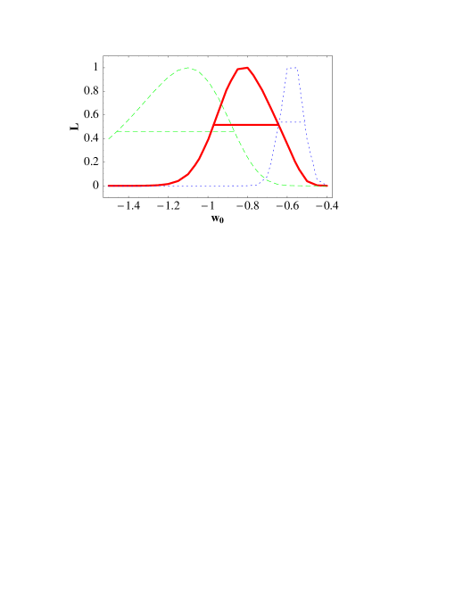
Figure 6: Likelihood for $w$ marginalized on $\Omega_{R}$, with priors in three different intervals. Full curve: $\Omega_{R}\in(0.04,0.3)$, flat prior. Dotted curve: $\Omega_{R}\in(0.04,0.06)$, flat prior. Dashed curve: $\Omega_{R}\in 0.3\pm 0.05$, Gaussian prior. The peak moves to $w>-1$ when $\Omega_{R}$ is smaller than 0.3. The horizontal lines mark the 68% confidence interval.

In conclusion, we have shown that from the analysis of recent SNe Ia there is still some room for strongly coupled dark energy scenarios which can ease the coincidence problem, and are compatible with an earlier beginning of the accelerated regime. Although more conventional models fit better the data, they seem to point toward a $w<-1$ equation of state for the cosmic dark energy component. If this tendency is confirmed by future observations we will face the problem of a theoretical interpretation of such a strong negative pressure. “Phantom” models, in fact, seem to be plagued with severe quantum instabilities. Coupled dark energy models, in this respect, could provide an interesting alternative.

We found that the “minimal model” in which only the baryons are uncoupled fits the SNe Ia at 2$\sigma$ if we restrict to $w>-1$, and at roughly 98% c.l. if we include the region $w<-1$. In both cases the best fit for the equation of state is $w=-0.6\pm 0.1$. The universe may start the present acceleration at a very early epoch, $z\approx 3$, much earlier than any uncoupled model. If some fraction of dark matter is let to be uncoupled as well, then the fit improves steadily as the fraction increases, but at the price of a large coupling $\beta$, which in turn induces potentially harmful violations of universality at the level of large scale gravitational interactions. A modest increase in the data statistics could definitely reject the minimal model of coupled dark energy, thus forcing an admixture of coupled and uncoupled dark matter as an acceptable cosmological scenario.

Acknowledgments. We are very grateful to Gabriele Veneziano for many helpful suggestions, and for a fruitful collaboration during the early stages of this work.

References

- [1] S. Perlmutter et al., Nature 391, 51 (1998); A. G. Riess et al., Astron. J. 116, 1009 (1998); P. de Bernardis et al., Nature 404, 955 (2000); S. Hanay et al., Astrophys. J. Lett. 545, L5 (2000); N. W. Alverson et al., Astrophys. J. 568, 38 (2002); D. N. Spergel et al., Astrophys. J. Suppl. 148, 175 (2003).
- [2] P. Steinhardt, in Critical problems in Physics, edited by by V. L. Fitch and D. R. Marlow (Princeton University Press, Princeton, NJ, 1997).
- [3] L. P. Chimento, A. S. Jakubi and D. Pavon, Phys. Rev. D 62, 063508 (2000); W. Zimdahl, D. J. Schwarz, A. B. Balakin and D. Pavon, astro-ph/0009353; S. Sen and A. A. Sen, Phys. Rev. D 63,124006 (2001); A. A. Sen and S. Sen, gr-qc/0103098; W. Zimdahl and D. Pavón, astro-ph/0105479
- [4] L. Amendola, Phys. Rev. D 62, 043511 (2000); L. Amendola and D. Tocchini-Valentini, Phys.Rev. D 64, 043509 (2001); L. Amendola and D. Tocchini-Valentini, Phys.Rev. D 66, 043528 (2002) .
- [5] L. Amendola, M. Gasperini, D. Tocchini-Valentini and C. Ungarelli, Phys.Rev. D 67, 043512 (2003); L. Amendola, Mon. Not. R. Astron. Soc. 342, 221 (2003); M. Gasperini, hep-th/0310293, in Proc. of the Int. Conf. on Thinking, Observing and Mining the Universe, Sorrento 2003, eds. G. Longo and G. Miele (World Scientific, Singapore), in press.
- [6] D. Comelli, M. Pietroni and A. Riotto, Phys. Lett. B 571, 115 (2003); U. Franca and R. Rosenfeld, astro-ph/0308149; A. V. Maccio et al. Phys. Rev. D 69, 123516 (2004).
- [7] G. Huey and B. D. Wandelt, astro-ph/0407196.
- [8] M. Gasperini, F. Piazza and G. Veneziano, Phys. Rev. D 65, 023508 (2002).
- [9] F. Piazza and S. Tsujikawa, JCAP 0407, 004 (2004).
- [10] G. Veneziano, JHEP 0206, 051 (2002).
- [11] G. R. Farrar and P. J. E. Peebles, Astrophys. J 604, 1 (2004).
- [12] M. Doran and J. Jaeckel, Phys. Rev. D 66, 043519 (2002).
- [13] We thank G. Veneziano for pointing out to our attention a comment by G. Dvali concerning radiative corrections to the mass of a coupled scalar.
- [14] S. S. Gubser and P. J. E. Peebles, hep-th/0407097.
- [15] A. G. Riess et al., astro-ph/0402512.
- [16] S. Hamestad and E. Morstel, Phys. Rev. D 66, 063508 (2002); A. Melchiorri et al., Phys. Rev. D 68, 043509 (2003).
- [17] R. R. Caldwell, Phys. Lett. B 545, 23 (2002); C. Armendariz-Picon, V. Mukhanov and P. J. Steinhardt, Phys. Rev. Lett. 85, 4438 (2000).
- [18] S. M. Carroll, M. Hoffman and M. Trodden, Phys. Rev. D 68, 023509 (2003); J. M. Cline, S. Y. Jeon and G. D. Moore, hep-ph/0311312.
- [19] V. K. Onemli and R. P. Woodard, Class. Quant. Grav. 19, 4607 (2002); V. K. Onemli and R. P. Woodard gr-qc/0406098.
- [20] E. J. Copeland, A. R. Liddle and D. Wands, Phys. Rev. D 57, 4686 (1998).
- [21] B. A. Gradwohl and J. A. Frieman, Astrophys. J. 398, 407 (1992).
- [22] L. Amendola et al., in preparation.
- [23] B. A. Bassett, P. S. Corasaniti and M. Kunz, astro-ph/0407364.
- [24] A. G. Riess et al., Astrophys. J. 560, 49 (2001).