Asteroseismology of exoplanets hosts stars : tests of internal metallicity

Exoplanets host stars present a clear metallicity excess compared to stars without detected planets, with an average overabundance of 0.2 dex. This excess may be primordial, in which case the stars should be overmetallic down to their center, or it may be due to accretion in the early phases of planetary formation, in which case the stars would be overmetallic only in their outer layers. In the present paper, we show the differences in the internal structure of stars, according to the chosen scenario. Namely two stars with the same observable parameters (luminosity, effective temperature, outer chemical composition) are completely different in their interiors according to their past histories, which we reconstitute through the computations of their evolutionary tracks. It may happen that stars with an initial overmetallicity have a convective core while the stars which suffered accretion do not. We claim that asteroseismic studies of these exoplanets host stars can give clues about their internal structures and metallicities, which may help in understanding planetary formation.

1 Introduction

Since the historical discovery of the first exoplanet by Mayor et al mayor95 (1995), more than one hundred and fifteen of these objects have presently been detected (Mayor mayor03 (2003), Santos et al santos04 (2004)). Due to technical limitations, the systems which have been observed are quite different from the solar system. They usually consist in a solar-type star surrounded by one or several Jupiter-like planets, orbiting at a short distance of the parent star.

A striking observation about exoplanets host stars concerns their metallicities which, on the average, are larger than those of stars without detected planets, by 0.2 dex (e.g. Gonzalez gonzalez97 (1997), Gonzalez gonzalez98 (1998), Santos et al. santos01 (2001), santos03 (2003) and santos04 (2004), Murray et al. murray01 (2001), Martell & Laughlin martell02 (2002)). The origin of this overmetallicity is still a subject of debate and is directly related to the process of planetary formation.

Two extreme scenarios have been proposed to account for this observed overmetallicity : we discuss them separately although it is not excluded that they both occur together in the same stars. The first one assumes that the stellar systems with planets were formed out of an already metal-rich protostellar gas (see Santos et al. santos04 (2004) for a recent review on the subject). The subjacent idea is that a larger metallicity helps forming planets as it implies a larger density of grains and more frequent collisions among heavy particles. As a consequence it becomes easier for planetesimal to form and accrete matter (e.g. Pollack et al. pollack96 (1996))

The second scenario assumes no difference of metallicity in the protostellar gas. In this case the metallicity excess would be due to the accretion of newly formed planets in the early phases : due to their interaction with the disk, the planets may migrate towards the star and eventually fall on it. Evidences of planet migration come from the mere observation of giant planets close to the central stars : the formation scenarios assume that they have been formed further away and have spiralled down due to their interaction with the disk (e.g. Trilling et al trilling98 (1998)). The basic difficulty is to understand the reason why the migration stops : it must be due to the absence of disk matter close to the star, which may be related to different effects. Within this framework, the accretion of some planets in the early epochs seems quite plausible. It may also be supported by the presence of ⁶Li in parent stars (Israelian et al israelian01 (2001), israelian04 (2004)). As they are mostly composed of heavy elements, the accretion of these planets should increase the metallicity of the star in its outer layers (Murray et al murray01 (2001)). However the number of planets needed to explain an overmetallicity by 0.2 dex is large : a $3M_{\oplus}$ terrestrial planet which could explain the ⁶Li/⁷Li ratio in HD82943 would increase the metallic abundance of the star by only $\simeq 17\%$ (Israelian et al israelian04 (2004)). Of course this depends on the chemical composition of the planets, but an increase of the metallicity as observed would need that the stars swallow several tens of earths, which is not completely excluded but seems very high.

A strong argument against the accretion scenario was raised by Santos et al santos01 (2001), who pointed out that similar accretion rates on main sequence stars should lead to a metal excess larger for stars with larger masses, as their convective zones are shallower (e.g. Pinsonneault et al pinsonneault01 (2001)). On the contrary, the observations show similar overmetallicities for stars of various effective temperatures. However this argument did not take into account double-diffusive convection, which should partially mix the accreted matter below the convective zone (Vauclair vauclair04 (2004)). Also accretion could occur before the zero age main sequence, in which case the convective zones are deeper.

Another argument has been used in favour of the primordial scenario : the existence of a correlation between the frequency of planets and the metallicity ; the more metal rich is the star, the larger is the probability of finding planets in orbit around it (e.g. Santos et al santos04 (2004)). This argument could however be used as a support of the accretion scenario as well : if many planets form around a star, the number of accreted ones is larger and the metallicity higher ; meanwhile the probability for the existence of an observable planet is also larger in this case.

In the present paper, we suggest to use asteroseismology of exoplanets hosts stars to check whether they are overmetallic down to their center (“overmetallic models”) or only in their outer layers (“accretion models”), which may help chosing between the two scenarios and lead to a better understanding of planetary formation.

Helioseismology has proved to be a powerful tool for solar physics, even for the detection of very small variations in the internal chemical composition (e.g. Bahcall et al bahcall92 (1992), Christensen-Dalsgaard et al jcd96 (1996), Richard et al. richard96 (1996), richard04 (2004), Brun et al brun98 (1998), Turcotte et al turcotte98 (1998)). Asteroseismology is now taking its turn and is expected to lead to major advances in stellar physics. The technics are different for the stars and for the Sun as the stars are always seen globally while the solar surface can be locally analysed. Contrary to the Sun, only modes with low $l$-degree values may be detected in stars (from 0 to 3 with the present asteroseismic technics). Even with such low degree modes, important clues can be obtained for the internal structure of the stars. Ground-based and space instruments (ELODIE, HARPS, MOST) are able to observe oscillations of solar-type stars. In the future, more precise observations are still expected from new missions like CoROT and possibly Eddington.

A good example of such asteroseismic studies is the detection of acoustic modes in $\alpha$Cen A (Bouchy & Carrier bouchy01 (2001)) using the ELODIE spectrograph in Haute Provence Observatory. Twenty eight modes of low degrees, ($l=0,1,2$) and radial orders between 15 and 25 were identified (Bouchy & Carrier bouchy02 (2002)). These oscillation frequencies were used to provide an accurate description of the internal physics of the star (Thevenin et al thevenin02 (2002), Thoul et al. thoul03 (2003), Eggenberger et al. eggenberger04 (2004)).

In the present paper, we compute stellar models for the overmetallic and accretion cases, which are iterated so that they converge on the same “observable” parameters (here we use $L,T_{eff}$ and chemical composition). The stars could not be differentiated by classical observation, but we will show that they are quite different in their internal structure and that the differences can be tested with asteroseismology.

The computations and computational parameters of the models are described in section 2. Two couples of models which are similar in their external parameters but with different histories and internal structures are defined in section 3 : their differences are analysed in details. Section 4 is devoted to the asteroseismic signatures of these differences. The results are summarized and discussed in section 5.

2 The computations

2.1 The physical parameters

The stellar models were computed with the Toulouse-Geneva code, including the most recent improvements in the physical inputs : new OPAL equation of state (Rogers & Nayfonov, rogers02 (2002)) ; NACRE nuclear reaction rates (Angulo et al., angulo99 (1999)) ; OPAL opacities (Iglesias & Rogers iglesias96 (1996)). Microscopic diffusion was included in all the models as described in Richard et al richard04 (2004). The convective zones were computed in the framework of the mixing length theory, with a mixing length parameter calibrated on the Sun and identical in all models : $\alpha=1.895$. No overshoot neither mixing were introduced in the present paper : their effects will be treated in a forthcoming paper. The oscillation frequencies of the models were computed using the Brassard et al. adiabatic pulsation code (brassard92 (1992)).

Evolutionary tracks (including standard pre main-sequence) were computed for stars with initial solar abundances (see table 1) modified by accretion in its outer layers (accretion models) and for stars with initial metallic excess (overmetallic models)

2.2 The accretion scenario

The accretion scenario assumes that the star is overmetallic only in its outer layers. This could be due to planetary material falling onto the star. We do not discuss here detailed scenarios for the accretion of planets, planetesimals or planetary material through evaporation. We assume, for a first approach, that the accreted matter has no hydrogen neither helium, while the other elements are present in solar relative abundances (this assumption can be tested by spectroscopy when applied to a real star). Also the accretion process is treated as instantaneous compared to the evolution time scale and is assumed to take place on the ZAMS. Except for hydrogen and helium, we set the surface abundances at the time of zero age main sequence as $X^{a}_{i}=X_{i}(1+f_{a})$ where f_a is a free parameter linked to the accreted mass. The hydrogen and helium mass fraction are then recomputed such that their ratio remains unchanged.

The effect of accretion on a standard model with solar initial abundances is shown in Fig. 1. We can see that the models with accretion are cooler than those without accretion which have the same internal abundances.

Figure 1: Evolutionary tracks for main sequence models of 1.1 M_⊙ without accretion (dashed line) and with accretion (full line). The symbols on each track correspond to ages of 30 Myr (asterix), 1 Gyr (diamonds), 4 Gyr (triangles) and 6 Gyr (squares). Here the comparisons are given for two models with the same internal chemical composition. We can see how accretion moves the tracks towards smaller effective temperatures. In the following we will compare models with the same external chemical composition and different internal structure.

2.3 The primordial scenario

The primordial scenario assumes that the star and the planets were formed out of initially overmetallic gas. This suggests that interstellar clouds inside the Galaxy may have metallic abundances varying by a factor of order two. We do not know however the helium abundance in such clouds. A possible assumption would be that it follows the regression law found for extragalactic HII regions, namely :

$$Y=Y_{p}+Z\frac{\Delta Y}{\Delta Z}$$ (1)

where Y_p is the primordial helium ratio and $\frac{\Delta Y}{\Delta Z}$ the slope of the regression curve obtained from observations (Isotov & Thuan isotov04 (2004)).

But the chemical history of intersellar clouds may be different from the overall chemical evolution of galaxies as the average stellar mass fraction may not be the same. In this case it is possible that helium remains solar while the metal abundances increase.

In the first case, the helium value for a metal increase by a factor 2 compared to the Sun would be Y=0.33 while in the second case it would remain Y=0.27 as in the Sun. The two cases have been treated in our computations as two possible extreme values.

2.4 Evolutionary tracks

Figs. 2 and 3 present evolutionary tracks for accretion and overmetallic models, for a selection of stellar masses. In Fig. 2 the overmetallic models have a helium abundance Y=0.27 while in Fig. 3 the helium abundance is Y=0.33. The accretion models are the same in both figures. The effective temperature scale is different. In each figure we can see that the behavior of the evolutionary tracks is quite different for accretion and overmetallic models. The models which have a metal excess down to their center have a convective core while the accretion models do not. Also a comparison between the two figures show that the overmetallic stars which also present a helium excess are hotter than those with a solar helium abundance.

Thus, to obtain the same external parameters (L, T_eff and metallicity), with the same Y₀ and $\alpha$, we expect that an overmetallic star will have a larger mass than a star which has suffered accretion. This fact has two major consequences which will be discussed later. First the internal structures of the stars are quite different and can hopefully be distinguished with asteroseismic studies ; second the determination of the masses of exoplanets may have to be reviewed if their host star is heavier than previously assumed.

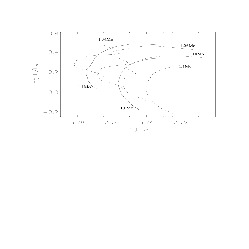
Figure 2: Evolutionary tracks for overmetallic (dashed lines) and accretion (full lines) models. In these computations, the overmetallic models have initial values : Z=0.04 and Y=0.27 while the accretion models have initial values Z=0.02 (increased to 0.04 in the outer layers at the beginning of the main sequence, due to accretion) and Y=0.27. For the overmetallic models, the tracks are plotted, from right to left, for the following masses : 1.1, 1.18, 1.26, and 1.34 M_⊙. For the accretion models, the tracks are plotted for 1.0 and 1.1 M_⊙.

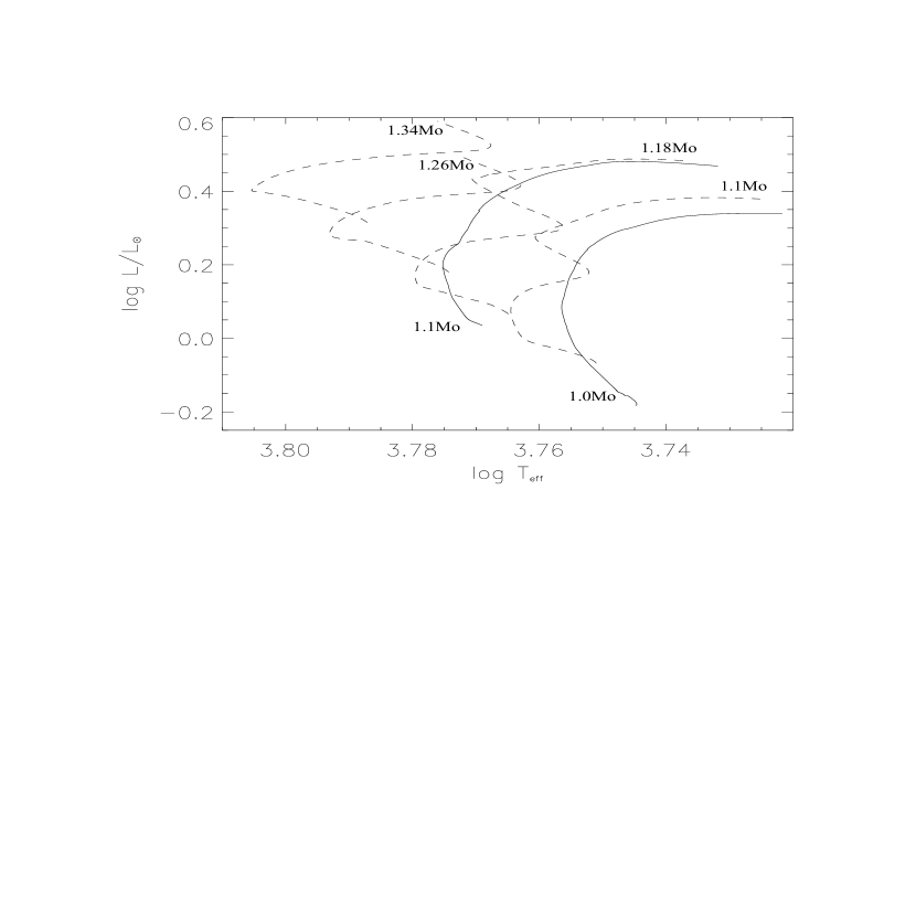
Figure 3: Same as Fig. 2, except that here the overmetallic models have initial values : Z=0.04 and Y=0.33

.

3 Comparisons of overmetallic and accretion models with similar external parameters

3.1 The models

We have computed evolutionary tracks for models with an initial overmetallicity and models with accretion. We chose to analyse two couples of models obtained with the same evolutionary track for the case of accretion, but two different tracks for the overmetallic case : one with an initial helium value $Y_{0}=0.27$ (they are called AC1 and OM1) and the second one with $Y_{0}=0.33$ (AC2 and OM2). The evolutionary tracks and the position of these models in the HR diagram are displayed on Fig. 4. As the aim of our computations was to compute models with similar external observable parameters, the evolutionary tracks correspond to different masses : $1.3M_{\odot}$ and $1.15M_{\odot}$ respectively for the overmetallic models, compared to $1.1M_{\odot}$ for the pulluted ones. A striking point is that a convective core develops in the overmetallic models, which gives the corresponding characteristic shape to the evolutionary track. On the other hand, the models with solar internal abundances which lie at the same position in the HR diagram do not develop any convective core.

The masses of the models are given in Table 1 together with their ages, and their initial and final surface chemical compositions. Table 2 shows the effective temperatures, luminosities, radii, surface gravities, acoustic depths of the models (i.e. time needed for the acoustic waves to travel along the stellar radius), as well as the geometrical and acoustic depths of the outer convective zones and the geometrical and acoustic radii of the convective cores if any. For an external observer, the stars are very similar inside each couple. The relative differences for T_eff and $\frac{L}{L_{\odot}}$ are very small : respectively of order $10^{-5}$ and $10^{-4}$. The metallicity is more difficult to match exactly because of element diffusion along the evolutionary tracks : the relative difference is $7\%$ for models AC1 and OM1 and $4\%$ for models AC2 and OM2. In each case the differences between the models are not detectable through classical spectroscopic observations. Their internal structures are however very different, as seen below.

Table 1: Masses, ages and chemical composition of the stellar models. X₀, Y₀ and Z₀ are the initial surface mass fractions of H, He and metals while X, Y and Z are the final ones.

Model	M⋆	Age (Gyr)	X0	Y0	Z0	X	Y	Z
AC1	1.1	5.578	0.7097	0.2714	0.0189	0.7478	0.2137	0.00385
OM1	1.3	3.623	0.6844	0.2714	0.0442	0.7221	0.2366	0.0413
AC2	1.1	3.290	0.7097	0.2714	0.0189	0.7287	0.2310	0.00403
OM2	1.15	2.771	0.6260	0.3297	0.0443	0.6589	0.2993	0.00418

Table 2: Output parameters of the models : effective temperature, luminosity, radius, surface gravity, total acoustic depth, geometrical and acoustic depth of the outer convective zone, geometrical and acoustic radius of the convective core (if any).

Model	Teff (K)	$\frac{L}{L_{\odot}}$	R⋆ (cm)	g (g.cm-2)	t⋆ (s)	$\frac{R_{ec}}{R_{\star}}$	$\tau_{ec}$	$\frac{R_{cc}}{R_{\star}}$	$t_{cc}$
AC1	5902.36	2.029	9.50e10	16146	5300.6	0.7211	3407	-	-
OM1	5902.48	2.030	9.50e10	19067	4900.9	0.7397	3056	0.0671	124.4
AC2	5959.03	1.555	8.16e10	21881	4254.5	0.7369	2760	-	-
OM2	5959.36	1.555	8.16e10	22880	4162.6	0.7191	2566	0.0655	102.5

Figure 4: Evolutionary tracks for accretion models (full lines) and overmetallic models (dashed lines) ; in both graphs, the accretion models have a mass of 1.1 M_⊙ and a solar composition inside (see Table 1) ; in graph a., the overmetallic models have a mass of 1.3 M_⊙ and an initial helium mass fraction Y₀=0.27 (solar like) ; in graph b., the overmetallic models have a mass of 1.15 M_⊙ and an initial helium mass fraction Y₀=0.33. The crosses identify the models AC1 and OM1 (a.), and AC2 and OM2 (b.)

3.2 Internal structure and chemical composition

For each couple, the overmetallic model has a convective core, contrary to the accretion model. Figures 5 and 6 display the relative differences of the internal density, pressure, temperature and square sound velocity in the two couples of models as a function of the fractional radius. For a given variable x, the adopted notation is $\frac{\Delta x}{x}=\frac{x_{OM}-x_{AC}}{x_{AC}}$ where OM and AC stand respectively for “overmetallic” and “accretion”. We can see that the differences are large, and the positions of the convective cores in the overmetallic models are clearly seen in the sound velocity graph.

Figures 7 and 8 display the internal chemical composition of the models. Figure 7 presents the abundance profiles of H, He, C, N, O, Ne, Mg and the heavier metals gathered in label Z for models AC1 and OM1. Fig. 8 presents the same graphs for models AC2 and OM2. The differences between the overmetallic and accretion models are clearly visible on these graphs.

Figure 5: Relative differences in density, pression, temperature and square of the sound speed between models AC1 and OM1. For any variable x, the ratio $\frac{\Delta x}{x}$ is defined as $\frac{x_{OM1}-x_{AC1}}{x_{AC1}}$.

Figure 6: Same as Fig.5, for models AC2 and OM2.

Figure 7: Mass fractions of H, He, C, N, O, Ne, Mg and Z(which includes all the heavier elements), as a function of the fractional radius, in models AC1 (full lines) and OM1 (dashed lines).

Figure 8: Same as Fig.7 for models AC2 and OM2.

3.3 Pulsation diagram

Figure 9 presents the pulsation diagram for each model. The Brunt-Väisälä frequency $N$ is plotted together with the Lamb frequency S_l for $l=1,2,3$ , as a function of the fractional radius. They were computed using the classical formulae :

$$N^{2}=\frac{g}{H_{p}}\left(\nabla_{ad}-\nabla_{rad}+\nabla_{\mu}\right)$$ (2)

$$S^{2}_{l}=l(l+1)\frac{c^{2}}{r^{2}}$$ (3)

Horizontal lines are schematically drawn in Fig. 9, for frequencies of 1 mHz and 2.5 mHz, down to the curves $l=1$, to help visualize the resonant acoustic cavities. The negative values of N² correspond to the region in which the medium is unstable against convection.

Figure 9: Pulsation diagrams for AC1 (a), OM1 (b.), AC2 (c.), OM2 (d.). The full lines represent the Brunt-Väisälä frequency, the dashed lines represent the Lamb frequency for $l=1,2,3$. Horizontal lines are drawn in each graphs for frequencies of 1 mHz and 2.5 mHz to help visualize the acoustic cavities.

4 Asteroseismic tests

For each model the oscillation frequencies were computed for p-modes of degrees $l=0$ to $l=3$. We then studied in detail the different combinations of these frequencies which could lead to observational tests of the internal structure and chemical composition of the stars.

4.1 Large separations

The “large separations” represent the frequency differences between two modes of the same degree $l$ and successive radial numbers $n$ :

$$\Delta\nu_{n,l}=\nu_{n,l}-\nu_{n-1,l}$$ (4)

For p-modes, the large separations are nearly constant, with values close to the fundamental asteroseismic quantity $\nu_{0}=1/2t_{\star}$, where $t_{\star}$ is the stellar acoustic radius (Table 2) (e.g. Audard & Provost audard94 (1994)).

Figures 10 and 11 display the ratio of the large separations for the four models, divided by $\nu_{0}$.

Figure 10: Large separations devided by $\nu_{0}$, inverse of twice the acoustic radius of the star, for models OM1 and AC1.

Figure 11: Large separations devided by $\nu_{0}$, inverse of twice the acoustic radius of the star, for models OM2 and AC2.

4.2 Small separations

We define the “small separations” as Roxburgh & Voronstsov roxburgh01 (2001):

$$D_{n,l}=\frac{\nu_{n,l}-\nu_{n-1,l+2}}{2l+3}$$ (5)

The repercussion of the presence of a convective core on the small separations have been studied by several authors (Provost et al provost93 (1993), Audard, Provost and Christensen-Dalsgaard audard95 (1995), Roxburgh & Voronstsov roxburgh01 (2001)). The boundary of the convective core induces a sharp variation in the sound velocity which leads to a partial reflexion of the waves which would otherwise travel down to the stellar center. Roxburgh & Vorontsov roxburgh01 (2001) have computed the oscillatory perturbations which appear in this case in the small separations. They exhibit a modulation with a period close to the acoustic radius of the core (time needed for the waves to travel between the stellar center and the core boundary) (Table 2). The oscillations have opposite phases for $l=0$ and $l=1$. When the effect of gravity perturbations is taken into account, this acoustic radius has to be replaced by an “effective acoustic radius” given by :

$$\tilde{t}=\int_{t_{1}}^{t}\left(1+\frac{G\rho_{0}}{\pi\nu^{2}}\right)^{\frac{1}{2}}dt=\int_{r_{1}}^{r}\left(1+\frac{G\rho_{0}}{\pi\nu^{2}}\right)^{\frac{1}{2}}\frac{dr}{c}$$ (6)

Roxburgh & Vorontsov roxburgh01 (2001) have shown that the best parameter to test the presence of a convective core is indeed the ratio of the small to the large separations, namely $R_{n,l}=\frac{\pi}{2}\frac{D_{n,l}}{\Delta\nu_{n,l}}$, as it helps getting rid of the surface effects on the frequencies. Unfortunately, the characteristic oscillations “periods” (in frequency units) are larger than the atmospheric cut-off frequency, so that only part of one oscillation can be visible from observations.

Figures 12 and 13 display the small separation for the four models, for $l=0$ and $l=1$ , up to frequencies of 10 mHz. In real stars the oscillation modes are only seen up to the cut-off frequency $\nu_{c}=\frac{c}{4\pi H_{p}}$ (Mazumdar & Antia mazumdar01 (2001)) which is indicated in the figures by a vertical line. The modulation is clearly seen in the overmetallic models, as well as the opposite phase between the modes of different degrees. Figures 14 and 15 present, for the four models, the parameter $R_{n,l}$ as a function of the frequencies, limited to 3 mHz which is a value close to the cut-off frequencies. This figure gives a clear idea of the values which may be obtained from the observations of stellar oscillations. We can see that, although only part of a modulation period is displayed, the oscillatory character of the ratio $R_{n,l}$ appears for the overmetallic models but not for the accretion models.

Figure 12: Small separation for models AC1 and OM1, for $l=0$ and $l=1$ , up to frequencies of 10 mHz. The vertical line corresponds to the cut-off frequencies. The oscillations due to the convective core are clearly seen for the overmetallic model. However they cannot be as clearly visible in real stars due to the cut-off frequencies.

Figure 13: Same as Fig.12 for models AC2 and OM2.

Figure 14: Parameter $R_{n,l}=\frac{\pi}{2}\frac{D_{n,l}}{\Delta\nu_{n,l}}$ , for models AC1 and OM1, up to $\nu$ = 3 mHz, close to the cut-off frequencies; The beginning of the oscillations is evident in the overmetallic model for $l=0$.

Figure 15: Same as Fig.14, for models AC2 and OM2

4.3 Second differences

Apart from their cores, overmetallic and accretion models also show some important differences in their outer layers. The most important is the presence of a steep $\mu$-gradient just below the convective zone of the accretion models. Also the sound velocities in the convective zones are larger by 2 to 5 % for the OM models compared to the AC models. Gough (gough90 (1990)) showed that rapid variations in the sound velocities in the outer layers of stars lead to oscillations which could be better seen in the so-called “second differences” $\delta_{2}\nu=\nu_{n+1}-2\nu_{n}+\nu_{n-1}$.

In the absence of chemical gradients, second differences are good indicators of the hydrogen and helium ionization zones, and of the base of the convective zone (Monteiro et al. monteiro94 (1994), Monteiro & Thompson monteiro98 (1998), Miglio et al miglio03 (2003)). When a helium gradient is present below the convective zone, it becomes the most effective “partial mirror” for the waves, leading to the most important modulation (Vauclair and Théado vauclair04b (2004)). On the other hand, the second differences are not influenced by the presence of a convective core (Mazumdar & Antia mazumdar01 (2001)).

Figures 16 and 17 present the second differences for the four models, as well as their Fourier transforms, while Figure 18 displays the usual thermodynamical parameter $\Gamma_{1}$ as a function of fractional radius. Three peaks are observed in the Fourier transforms. The two ones on the left, below times of 2000 s, correspond to the ionisation zones which lead to the drops and kinks in $\Gamma_{1}$. Each peak appears for a characteristic time which is twice the time needed for the sound waves to travel from the surface down to the considered layers. The third peak, around 6000 s, corresponds to the bottom of the convective zone, as can be checked from the acoustic depth given in Table 2. In each case, the acoustic depth of the convective zone, hence the position of the peak, corresponds to a larger time in the accretion models than in the overmetallic models. Here the helium gradients are not strong enough, nor the metallic gradients induced by accretion, to be seen in the second differences.

Figure 16: Second differences and Fourier transforms for models OM1 and AC1. The peaks below 2000 s are due to the helium ionisation zones while the peak around 6000 s is due to the bottom of the convective zone.

Figure 17: Same as Fig. 16 for models OM2 and AC2

Figure 18: Profiles of the thermodynamical parameter $\Gamma_{1}$ for models OM1 and AC1 (top), OM2 and AC2 (bottom). The kinks in $\Gamma_{1}$ are the reason for the two left peaks in Figs. 16 and 17, bottom graphs.

5 Discussion

We have studied two couples of models, each of them with identical outer (observable) parameters : $L,T_{eff}$, external chemical composition, but different histories. In each couple, one partner was a model with an overmetallicity down to the stellar center (overmetallic model) while the other partner was a model with normal (solar) composition with an metallicity increase in the external layers due to accretion (accretion model). In the first couple (models OM1 and AC1), the helium value was solar in the two partners, while in the second couple (models OM2 and AC2), the overmetallic model was assumed to have also an increase of helium, according to the Y-Z relation obtained for the chemical evomution of galaxies (Izotov & Thuan isotov04 (2004)).

We always considered that the accreted matter contained neither hydrogen nor helium. For the other elements, we assumed solar relative abundances. The accreted material was supposed to be instantaneously mixed in the convective zone at the beginning of the zero-age-main-sequence. For a first approach, double-diffusive mixing (Vauclair vauclair04 (2004)) was not introduced in the present computations. Models including this effect will be presented in a forthcoming paper.

We show that their are drastic differences between two models which would appear as the same star from outside, but which have different chemical composition inside. The overmetallic models have a larger mass than the accretion models, and the most important differences in their internal structure is that the first ones develop a convective core while the second ones do not. Also the outer convective zones do not have the same depth and there is a metallic gradient below the convective boundary in the accretion models.

We have investigated the possible asteroseismic tests of these differences. We found that the differences in the internal structure lead to signatures in the large separations (the acoustic radii of the stars are different), small separations and second differences. While the second differences can give the position of the bottom of the outer convective zone, the most important effect is seen in the ratio of the small to the large separations : an oscillatory behavior clearly related to the presence of the convective core is seen in the overmetallic models and does not exist in the accretion models.

These first results are very encouraging and we may hope to be able to derive, by observing real central stars of planetary systems, whether they are overmetallic down to the center or suffered planetary accretion. Such results would be very helpful to understand the formation of planetary systems.

- (1) Angulo C., Arnould M., Rayet M., (NACRE collaboration), 1999, Nuclear Physics A 656, 1, http://pntpm.ulb.ac.be/Nacre/nacre.htm
- (2) Audard, N., Provost, J., 1994, A&A, 297, 427
- (3) Audard, N., Provost, J., & Christensen-Dalsgaard, J., 1995, A&A, 297, 427
- (4) Bahcall, J. N., Pinsonneault, M. H., 1992, Rev. Mod. Phys. 64(4), 885
- (5) Bouchy, F. & Carrier, F., 2001, A&A, 374, L5
- (6) Bouchy, F. & Carrier, F., 2002, A&A, 390, 205
- (7) Brassard, P., 1992, Ap.JS., 81, 747
- (8) Brun A. S., Turck-Chièze S., Morel P., 1998a, ApJ 506, 913
- (9) Christensen-Dalsgaard J. et al., 1996, Science 272, 1286
- (10) Eggenberger, A., Charbonnel, C., Talon, S., Meynet, G., Maeder, A., Carrier, F. 2004, A&A, 417, 353
- (11) Gonzalez, G.,1997, MNRAS, 285, 403
- (12) Gonzalez, G., 1998, A&A, 334, 221
- (13) Gough, D.O., 1990, in Progress of Seismology of the Sun and Stars, proceedings of the Oji International Seminar Hakone, Japan, Springer Verlag, Lecture notes in Physics 367, p.283-318
- (14) Iglesias, C. A. & Rogers, F. J., 1996, Ap.J., 464, 943
- (15) Israelian, G., Santos, N. C., Mayor, M., Rebolo, R., 2001, Nature, 411, 163
- (16) Israelian, G., Santos, N. C., Mayor, M., Rebolo, R., 2001, A&A, in press (astro-ph/0304358)
- (17) Izotov, Thuan, 2004, Ap.J., 602, 200
- (18) Martell, S., Laughlin, G., 2002, Ap.J., 577, L45
- (19) Mayor, M. & Queloz, D., 1995, Nature, 378, 355
- (20) Mayor, M., 2003, in Extrasolar Planets : Today and Tomorrow, ed. C. Terquem, A. Lecavelier des Etangs, & J-P. Beaulieu, XIXth IAP Colloquium, in press
- (21) Mazumdar, A., Antia, H.M., 2001, A&A 377, 192
- (22) Miglio, A., Christensen-Dalsgaard, J., Di Mauro, M.P., Monteiro, M.J.P.F.G., Thompson, M.J. 2003, in Asteroseismology across the HR diagram ed. M.J. Thompson, M.S. Cunha, M.J.P.F.G. Monteiro, (Kluwer, Dordrecht) p. 537
- (23) Monteiro, M.J.P.F.G., Christensen-Dalsgaard, J., Thompson, M.J., 1994, A&A 283, 247
- (24) Monteiro, M.J.P.F.G., Thompson, M.J., 1998, in New eyes to see inside the Sun and stars, proceedings of the IAU symposium 185, ed F.-L. Deubner, J. Christensen- Dalsgaard, D.W. Kurtz (Kluwer, Dordrecht) p. 317
- (25) Murray, N., Chaboyer, B., Arras, P., Hansen, B., & Noyes, R. W., 2001, Ap.J., 555, 801
- (26) Paquette, C., Pelletier, C., Fontaine, G., & Michaud, G., 1986, Ap.J.s, 61, 177
- (27) Pinsonneault, M.H., DePoy, D.L., & Coffee, M., 2001, Ap.J., 556, 59
- (28) Pollack, J. B., Hubickyj, O., Bodenheimer, P., Lissauer, J. J., Podolak, M., & Greenzweig, Y., 1996, Icarus, 124, 62
- (29) Provost, J., Mosser, B., Berthomieu, G., 1993, A&A, 274, 595
- (30) Richard, O., Vauclair, S., Charbonnel, C., Dziembowski, W. A., 1996, A&A 312, 1000
- (31) Richard, O., Théado, S., Vauclair, S., 2004, Solar physics, in press
- (32) Rogers, F. J., Nayfonov, A., 2002, ApJ 576, 1064
- (33) Roxburgh, I. W. & Vorontsov, S. V., 1994, Mon. Not. R. Astron. Soc, 267, 297
- (34) Roxburgh, I. W. & Vorontsov, S. V., 2001, Mon. Not. R. Astron. Soc, 322, 85
- (35) Santos, N. C., Israelian, G., Mayor, M., 2001, A&A, 373, 1019
- (36) Santos, N. C., Israelian, G., Mayor, M., Rebolo, R., & Udry, S., 2003, A&A, 398, 363
- (37) Santos, N. C., Israelian, G., Mayor, M, 2004, A&A, 415, 1153
- (38) Thévenin, F., Provost, J., Morel, P., Berthomieu, G., Bouchy, F., & Carrier, F., 2002, A&A, 392, L9
- (39) Trilling, D.E., Benz, W., Guillot, T., Lunine, J.I., Hubbard, W.B., Burrows, A., 1998, Ap.J., 500, 428
- (40) Thoul, A., Scuflaire, R., Noels, A., Vatovez, B., Briquet, M., Dupret, M.-A., & Montalban, J., 2003, A&A, 402, 293
- (41) Turcotte, S., Richer, J., Michaud, G., Iglesias, C.A., Rogers, F.J., 1998, Ap.J., 504, 539
- (42) Vauclair, S., 2004, Ap.J., 000, 000
- (43) Vauclair, S., Théado, S. 2004, A&A, 000, 000