Observational constraints on patch inflation in noncommutative spacetime

Abstract

We study constraints on a number of patch inflationary models in noncommutative spacetime using a compilation of recent high-precision observational data. In particular, the four-dimensional General Relativistic (GR) case, the Randall-Sundrum (RS) and Gauss-Bonnet (GB) braneworld scenarios are investigated by extending previous commutative analyses to the infrared limit of a maximally symmetric realization of the stringy uncertainty principle. The effect of spacetime noncommutativity modifies the standard consistency relation between the tensor spectral index and the tensor-to-scalar ratio. We perform likelihood analyses in terms of inflationary observables using new consistency relations and confront them with large-field inflationary models with potential $V\propto\varphi^{p}$ in two classes of noncommutative scenarios. We find a number of interesting results: (i) the quartic potential ($p=4$) is rescued from marginal rejection in the class 2 GR case, and (ii) steep inflation driven by an exponential potential ($p\to\infty$) is allowed in the class 1 RS case. Spacetime noncommutativity can lead to blue-tilted scalar and tensor spectra even for monomial potentials, thus opening up a possibility to explain the loss of power observed in the cosmic microwave background anisotropies. We also explore patch inflation with a Dirac-Born-Infeld tachyon field and explicitly show that the associated likelihood analysis is equivalent to the one in the ordinary scalar field case by using horizon-flow parameters. It turns out that tachyon inflation is compatible with observations in all patch cosmologies even for large $p$.

I Introduction

Early-Universe observations have come to the golden age. The first-year results of the Wilkinson Microwave Anisotropy Probe (WMAP) ben03 ; spe03 ; pei03 provided high-precision cosmological dataset from which early-Universe models can be tested. The observations strongly support the inflationary paradigm based on General Relativity (GR) as a backbone of high-energy physics. In particular, nearly scale-invariant and adiabatic density perturbations generated in single-field inflation exhibit an excellent agreement with the observed cosmic microwave background (CMB) anisotropies pei03 ; bri03 ; BLM ; KKMR ; LL ; teg04 . Together with the upcoming high-precision data by the Planck satellite planc , it will be possible to discriminate between a host of inflationary models from observations.

From the theoretical side, there has been a lot of interest in the construction of high-energy models of the early Universe. This interest is motivated by string cosmology, an attempt to merge string theory and cosmology as a generalization of the standard inflationary paradigm based on GR. A well-known example is the Randall-Sundrum (RS) II braneworld scenario RS , in which our four-dimensional brane is embedded in a five-dimensional bulk spacetime (see, e.g., mar03 ; BVD ; cal3 for a list of references on this subject). The spectra of perturbations generated in braneworld inflation are modified due to the presence of the 5th dimension MWBH ; LMW , but the consistency equation relating the tensor-to-scalar ratio to the spectral index of tensor perturbations is unchanged HuL1 ; HuL2 . Nevertheless, observational constraints in terms of underlying potentials are different compared to the GR case LS ; TL . It was shown that the quartic chaotic potential ($V\propto\phi^{4}$) is under a strong observational pressure and that steep inflation driven by an exponential potential is ruled out. This situation changes if we account for the Gauss-Bonnet (GB) curvature invariant in five dimensions, arising from leading-order quantum corrections of the low-energy heterotic gravitational action (see Ref. LN for one of the first works about GB braneworld inflation). One effect of the GB term is to break the degeneracy of the standard consistency relation DLMS . Although this does not lead to a significant change for the likelihood results of the inflationary observables, the quartic potential is rescued from marginal rejection for a wide range of energy scales TSM . Even steep inflation exhibits marginal compatibility for a sufficient number of $e$-folds ($N\gtrsim 55$).

Another interesting string-inspired scenario is noncommutative inflation ABM ; BH in which the presence of a stringy spacetime uncertainty relation leads to the modification of perturbation spectra at large scales. The implications of maximally symmetric noncommutativity have been extensively studied, e.g., in Refs. HL1 ; FKM ; FKM2 ; TMB ; HL2 ; HL3 ; LiLi ; KLM ; KLLM ; Cai ; LMMP ; AN ; cal4 ; cal5 ; myu04 . Since the uncertainty relation is saturated when a perturbation with a particular wavelength is generated, the standard evolution of commutative fluctuations is altered and large-scale modes are suppressed. In Ref. TMB the CMB power spectrum was divided into three main regions, ultraviolet (UV), intermediate, and infrared (IR). It was also assumed that the perturbation spectra at low multipoles are generated between the UV and intermediate regimes to explain the loss of power observed in CMB anisotropies. In this case, however, the suppression of power is not significant since the intermediate spectrum is nearly scale invariant. In this work we will adopt another perspective, that is, to consider the far IR regime as a dominant contribution to the large-scale spectrum.

We implement both braneworld and noncommutative frameworks as well as the standard GR commutative/noncommutative paradigm. We place observational constraints on a number of models generated by different braneworld and noncommutative prescriptions. Using the patch framework cal3 coupled to the slow-roll (SR) formalism, we will derive consistency equations between the inflationary observables: the scalar ($n_{s}$) and tensor ($n_{t}$) indices, their runnings ($\alpha_{s}$ and $\alpha_{t}$), and the tensor-to-scalar ratio $R$. In particular, the consistency relation between $n_{t}$ and $R$ is modified by the effect of spacetime noncommutativity, which breaks the degeneracy of the consistency relation in the commutative GR/RS cases. We have a variety of consistency relations for each patch cosmology (see Table 2 in Sec. II). Our numerical analysis based on recent observational data shows that the general shape of likelihood contours in the $n_{s}$-$R$ plane is deformed independently by braneworld and noncommutative effects. The major modification to the GR/RS commutative cosmology appears for the upper bound of $R$, roughly setting it in a $2\sigma$ interval with $0.5\lesssim R_{\text{max}}\lesssim 0.7$. The scalar index always ranges $0.9<n_{s}<1.1$ at the $2\sigma$ level.

We also place constraints on monomial potentials $V=V_{0}\varphi^{p}$ (including the exponential potential by taking the limit $p\to\infty$) in GR/RS/GB cases in noncommutative spacetime. An intriguing feature is that the effect of the new physics allows a blue-tilted spectrum, thus giving rise to a variety of theoretical points in the $n_{s}$-$R$ plane. For example, steep inflation driven by an exponential potential is excluded in the commutative RS scenario, but the same potential can be compatible with observations in the IR noncommutative limit. We shall investigate the observational compatibility of each scenario in detail. The suppression of the power spectrum at low multipoles will also be discussed by using the IR blue-tilted spectrum.

In addition to the ordinary scalar inflation, we will consider the Dirac-Born-Infeld tachyon field. Soon after the first proposal by Gibbons gib02 , it became clear that the cosmology based upon a rolling tachyon suffers from a number of problems, including a difficulty of reheating and a large amplitude of density perturbations, that can be traced back to some fine-tuning requirements on the parameters of the model CGJP ; FKS ; KL ; SCQ ; BBS ; BSS ; PS ; rae04 (see also PCZZ ). Lately it was shown in Ref. GST that the problem of large density perturbations is solved by considering a small warp factor $\beta$ in a warped metric. In addition, the problem of reheating is overcome by accounting for a negative cosmological constant which may appear by the stabilization of modulus fields KKLT .

By the reasons presented above, it is premature to exclude tachyon inflation. In this work we will show that the likelihood analysis for the inflationary observables in the tachyon case is identical to that for the ordinary scalar field by expressing the observables in terms of horizon-flow parameters. We also place observational constraints on the large-field potentials in noncommutative GR/RS/GB cases. Remarkably, even steep inflation is within the $2\sigma$ contour bound in all cases because of a small tensor-to-scalar ratio.

The paper is organized as follows. In Sec. II we provide our general (non)commutative patch setup. In Sec. III we perform likelihood analysis using the latest observational data set. After computing the theoretical values of $n_{s}$ and $R$ for the potential $V=V_{0}\varphi^{p}$ in Sec. IV, these are confronted with the likelihood contour bounds in Sec. V. We give conclusions and discussion in Sec. VI.

II The models

Consider a four-dimensional Friedmann-Robertson-Walker (FRW) cosmological background in which the effective Friedmann equation is given by

$$H^{2}=\beta_{q}^{2}\rho^{q}\,,$$ (1)

where $H$ is the Hubble rate and $\beta_{q}$ and $q$ are constants. General relativity, Randall-Sundrum and Gauss-Bonnet braneworld cases correspond to $q=1$, $q=2$ and $q=2/3$, respectively. We shall investigate a situation in which a homogeneous scalar field, $\varphi$, is confined on the 3-brane. The field $\varphi$ plays the role of the inflaton which is responsible for the generation of primordial perturbations.

In this paper we are interested in two candidates for the inflaton $\varphi$. The first one is a standard minimally coupled scalar field, $\phi$, whose energy density is

$$\rho=\frac{1}{2}\dot{\phi}^{2}+V(\phi)\,,$$ (2)

where $V(\phi)$ is the potential of $\phi$. The inflaton satisfies the following equation of motion

$$\ddot{\phi}+3H\dot{\phi}+V^{\prime}=0\,,$$ (3)

where a prime denotes the $\phi$ derivative. The second one is a tachyon-type scalar field, $T$, with a Born-Infeld action. In this case the energy density is given by

$$\rho=\frac{V(T)}{\sqrt{1-\dot{T}^{2}}}\,,$$ (4)

together with the equation of motion

$$\frac{\ddot{T}}{1-\dot{T}^{2}}+3H\dot{T}+U^{\prime}=0\,,$$ (5)

where $U\equiv\ln V$ is differentiated with respect to $T$.

The SR parameters associated with the inflaton $\varphi$ are cal3

$$\epsilon_{\varphi} \equiv -\frac{\dot{H}}{H^{2}}\,,$$ (6a)

$$\eta_{\varphi} \equiv -\frac{d\ln\dot{\varphi}}{d\ln a}=-\frac{\ddot{\varphi}}{H\dot{\varphi}}\,,$$ (6b)

$$\xi_{\varphi}^{2} \equiv \frac{1}{H^{2}}\left(\frac{\ddot{\varphi}}{\dot{\varphi}}\right)^{\cdot}\,,$$ (6c)

where $\varphi=\phi,T$. For example, in the case of the normal scalar field $\phi$, we have

$$\epsilon_{\phi}=\frac{3q\beta_{q}^{2-\theta}}{2}\frac{\dot{\phi}^{2}}{H^{2-\theta}}\,,$$ (7a)

where

$$\theta=2\left(1-\frac{1}{q}\right)\,,$$ (8)

while for the tachyon

$$\epsilon_{T}=\frac{3q}{2}\dot{T}^{2}\,.$$ (9a)

Then $\epsilon_{\varphi}$ can be written as

$$\epsilon_{\varphi}=\frac{3q\beta_{q}^{2-\tilde{\theta}}}{2}\frac{\dot{\varphi}^{2}}{H^{2-\tilde{\theta}}}\,,$$ (10a)

where $\tilde{\theta}=\theta$ for $\varphi=\phi$ and $\tilde{\theta}=2$ for $\varphi=T$.

As we shall see below, it is convenient to introduce the horizon-flow (HF) parameters STG ; kin02 , defined by

$$\epsilon_{0}=\frac{H_{\rm inf}}{H}\,,\qquad\epsilon_{i+1}=\frac{d\ln|\epsilon_{i}|}{dN}\,,\qquad i\geq 0\,,$$ (11)

where $H_{\rm inf}$ is the Hubble rate at some chosen time and $N\equiv\ln(a/a_{i})$ is the number of $e$-folds; here $t_{i}$ is the time when inflation begins. The evolution equation for the HF parameters is given by $\dot{\epsilon}_{i}=H\epsilon_{i}\epsilon_{i+1}$. The HF parameters are related to the first SR parameters, as

$$\epsilon_{1} = \epsilon_{\varphi}\,,$$ (12a)

$$\epsilon_{2} = \big{(}2-\tilde{\theta}\big{)}\epsilon_{\varphi}-2\eta_{\varphi}\,,$$ (12b)

$$\epsilon_{2}\epsilon_{3} = \big{(}2-\tilde{\theta}\big{)}^{2}\epsilon_{\varphi}^{2}-2\big{(}3-\tilde{\theta}\big{)}\epsilon_{\varphi}\eta_{\varphi}+2\xi_{\varphi}^{2}\,.$$ (12c)

Noncommutative inflation arises when we impose a realization of the *-algebra on the brane coordinates; an algebra preserving the maximal symmetry is $[\tau,x]=il_{s}^{2}$, where $\tau\equiv\int a\,dt$, $x$ is a comoving spatial coordinate on the brane and $l_{s}\equiv M_{s}^{-1}$ is the fundamental string scale. Let us introduce the noncommutative parameter $\delta\equiv(M_{s}/H)^{2}$; the noncommutative algebra induces a cutoff $k_{0}(\delta)$ roughly dividing the space of comoving wave numbers into two regions, one encoding the UV, small-scale perturbations generated inside the Hubble horizon ($H\ll M_{s}$) and the other describing the IR, large-scale perturbations created outside the horizon ($H\gg M_{s}$). By definition, they correspond to the quasicommutative and strongly noncommutative regimes, respectively. It turns out that one can write the spectra of scalar and tensor perturbations in the form

$$A(\delta,\,H,\,\varphi)=A^{(c)}(H,\,\varphi)\,\Sigma(\delta)\,,$$ (13)

where $A^{(c)}=A(\Sigma\!\!=\!\!1)$ is the amplitude in the commutative limit and $\Sigma(\delta)$ is a function encoding leading-SR-order noncommutative effects.

Equation (13) is evaluated at the horizon crossing in the UV limit and at the time when the perturbation with comoving wavenumber $k$ is generated in the IR limit. To lowest order in the HF (or SR) parameters,

$$\frac{d\ln\Sigma^{2}}{d\ln k}=\sigma\epsilon_{1}\,,$$ (14)

where $\sigma=\sigma(\delta)$ is a function of $\delta$ such that $\dot{\sigma}=O(\epsilon_{1})$. The standard commutative spacetime corresponds to $\sigma=0$.

The amplitudes of scalar and tensor perturbations are given, respectively, by

$$A_{s}^{2}(\varphi) = \frac{3q\beta_{q}^{2-\theta}}{25\pi^{2}}\frac{H^{2+\theta}}{2\epsilon_{1}}\Sigma^{2}\,,$$ (15)

$$A_{t}^{2}(\varphi) = \frac{3q\beta_{q}^{2-\theta}}{25\pi^{2}}\frac{H^{2+\theta}}{2\zeta_{q}}\Sigma^{2}\,,$$ (16)

where the coefficient $\zeta_{q}$ in $A_{t}^{2}$ depends on the model one considers. The standard GR case corresponds to $\zeta_{1}=1$, whereas one has $\zeta_{2}=2/3$ for the RS braneworld LMW . In the GB case $\zeta_{2/3}=1$, as recently shown in Ref. DLMS .

The spectral indices of scalar and tensor perturbations are given by

$$n_{s}-1 \equiv \frac{d\ln A_{s}^{2}}{d\ln k}=-(2+\theta-\sigma)\epsilon_{1}-\epsilon_{2}\,,$$ (17)

$$n_{t} \equiv \frac{d\ln A_{t}^{2}}{d\ln k}=-(2+\theta-\sigma)\epsilon_{1}\,,$$ (18)

where we used $d\ln\,k\approx Hdt$; the effect of noncommutativity is encoded in the $\sigma$ term. The ratio of tensor-to-scalar perturbations is

$$R\equiv 16\frac{A_{t}^{2}}{A_{s}^{2}}=\frac{16\epsilon_{1}}{\zeta_{q}}\,.$$ (19)

Since the same factor $\Sigma$ multiplies both the tensor and scalar amplitudes, their ratio is unchanged with respect to the commutative case. We have $R=16\epsilon_{1}$ for the GR and GB cases and $R=24\epsilon_{1}$ for the RS case. The runnings of the spectral indices, $\alpha_{s,t}\equiv dn_{s,t}/d\ln k$, are given by

$$\alpha_{s} = -(2+\theta-\sigma)\epsilon_{1}\epsilon_{2}-\sigma\bar{\sigma}\epsilon_{1}^{2}-\epsilon_{2}\epsilon_{3}\,,$$ (20)

$$\alpha_{t} = -(2+\theta-\sigma)\epsilon_{1}\epsilon_{2}-\sigma\bar{\sigma}\epsilon_{1}^{2}\,,$$ (21)

where $\bar{\sigma}$ is defined as $\bar{\sigma}\equiv-\dot{\sigma}/(H\sigma\epsilon)$. If $\sigma$ is a constant, $\bar{\sigma}$ vanishes.

All the previous expressions can be combined into the (nonclosed) set of consistency equations:

$$n_{t} = -(2+\theta-\sigma)\frac{R\zeta_{q}}{16}\,,$$ (22)

$$\alpha_{s} = \frac{R\zeta_{q}}{16}\left\{(2+\theta-\sigma)(n_{s}-1)\vphantom{\frac{1}{1}}\right.$$ (23)

$$\quad\quad+\left.\left[(2+\theta-\sigma)^{2}-\sigma\bar{\sigma}\right]\frac{R\zeta_{q}}{16}\right\}-\epsilon_{2}\epsilon_{3}\,,$$

$$\alpha_{t} = \frac{R\zeta_{q}}{16}\left\{(2+\theta-\sigma)(n_{s}-1)\vphantom{\frac{1}{1}}\right.$$ (24)

$$\quad\quad+\left.\left[(2+\theta-\sigma)^{2}-\sigma\bar{\sigma}\right]\frac{R\zeta_{q}}{16}\right\}\,.$$

Notably these relations do not depend on which inflaton field one is assuming on the brane. This means that the likelihood analysis for the field $\phi$ in terms of the variables $n_{s}$, $R$ and $\epsilon_{3}$ with given values of $q$, $\sigma$ and $\bar{\sigma}$ is identical to the one for the tachyon $T$. Using the SR parameters given in (6a)–(6c), the running of the scalar perturbations would split into two different equations cal4 :

$$\alpha_{s}(\phi) = \frac{R\zeta_{q}}{16}\left\{\vphantom{\frac{1}{1}}(5-\sigma)(n_{s}-1)+[4(3+\theta)\right.$$ (25)

$$\quad\qquad-\left.\sigma(7+\theta+\bar{\sigma}-\sigma)]\frac{R\zeta_{q}}{16}\right\}-2\xi_{\text{\tiny$\phi$}}^{2},$$

$$\alpha_{s}(T) = \frac{R\zeta_{q}}{16}\left\{\vphantom{\frac{1}{1}}(3+\theta-\sigma)(n_{s}-1)+[(2+\theta)(3+\theta)\right.$$ (26)

$$\quad\qquad\left.-\sigma(5+2\theta+\bar{\sigma}-\sigma)]\frac{R\zeta_{q}}{16}\right\}-2\xi_{\text{\tiny$T$}}^{2};$$

then one would need to perform two separate likelihood analyses. In this sense, the HF parameters are a more convenient choice for numerical purposes than the SR parameters.

The consistency relation (22) yields $n_{t}=-(2+\theta)\zeta_{q}R/16$ in the commutative spacetime ($\sigma=0$). Then we have $n_{t}=-R/8$ for the GR and RS cases, while the GB case, corresponding to $n_{t}=-R/16$, breaks this degeneracy DLMS .

One can “deform” the consistency equations by taking the spacetime noncommutativity into account ($\sigma\neq 0$). Two classes of noncommutative models have been found in the infrared region BH . In the first one (class 1), the FRW 2-sphere is factored out in the measure of the effective 4D perturbation action $z_{k}$, which is given by the product of the commutative measure $z$ and a correction factor of the $1+1$ noncommutative model. In the class 2 choice, the scale factor in the measure is everywhere substituted by an effective scale $a_{\text{\tiny eff}}$ whose time dependence is smeared out by the nonlocal physics; since $z\propto a$, then $z_{k}=za_{\text{\tiny eff}}/a$. Inequivalent prescriptions on the ordering of the *-product in the perturbation action further split these two classes, but in the IR limit they give almost the same predictions cal4 .

Since $\sigma$ is a nontrivial function of the noncommutative parameter, the space of the cosmological observables is enlarged, thus modifying the determination of the constraints from observations. However, in the far IR limit this function approaches a constant value, $\sigma=6$ in class 1 models and $\sigma=2$ in class 2 models. For positive values of $\sigma$ the perturbation spectra tend to be blue tilted in the IR region relative to the UV commutative case. For example, in the GR class 1 IR case ($\theta=0$ and $\sigma=6$), we have $n_{s}-1=4\epsilon_{1}-\epsilon_{2}$ and $n_{t}=4\epsilon_{1}>0$ by Eqs. (17) and (18), which means that the spectrum of gravitational waves is always blue tilted. Tables 1 and 2 summarize the scenarios we are going to explore. For later convenience we dub the commutative spacetime ($\sigma=0$) as “class 0.” We find that the quantity $n_{t}/R$ is always positive in the class 1 IR case. Thus, the introduction of noncommutativity breaks the standard GR commutative consistency relation $n_{t}=-R/8$ in a variety of ways.

Table 1: The values of $q$, $\theta$ and $\zeta_{q}$ for each patch inflation.

	$GR$	$RS$	$GB$
$q$	$1$	2	2/3
$\theta$	$0$	1	$-1$
$\zeta_{q}$	$1$	2/3	1

Table 2: The consistency equation (22) in the commutative UV and noncommutative IR limit.

(Non)commutative	$\sigma$	$n_{t}/R$
models		$GR$	$RS$	$GB$
Class 0 UV	$0$	$-1/8$	$-1/8$	$-1/16$
Class 1 IR	$6$	$1/4$	$1/8$	$5/16$
Class 2 IR	$2$	$0$	$-1/24$	$1/16$

III Likelihood analysis for noncommutative inflation

In Ref. TMB , a large-scale power spectrum was derived in the context of power-law inflation for an IR mode generated around $\tau\approx k_{0}l_{s}^{2}$. If this spectrum corresponds to the scale around $1<\ell\lesssim 10$, then the cosmologically relevant modes with $10\lesssim\ell\lesssim 1000$ also belong to the same IR spectrum. This is because the characteristic scale of this spectrum is $k_{s3}=10^{-5}k_{s2}$, where $k_{s2}$ is an intermediate scale around which the IR description becomes invalid [see Eq. (12) of TMB ]. In Ref. TMB it was assumed that the intermediate spectrum dominates at largest scales ($1<\ell\lesssim 10$), following the approach of Ref. HL1 . In this work we shall investigate a situation in which the IR spectra $\Sigma^{2}\sim\delta^{3}$ [class 1, which is Eq. (23) of Ref. TMB in the de Sitter limit] and $\Sigma^{2}\sim\delta$ (class 2) correctly describe the large-scale sector with $1<l\lesssim 10$. Since one generally has $k_{s2}\gg k_{s3}$, it is natural to use the IR power spectrum over the cosmologically relevant scales with $1<\ell\lesssim 2000$.

We have run the Cosmological Monte Carlo CosmoMC code together with the CAMB program LCS ; LB ; camb , applied to the latest observational data coming from the dataset of WMAP wmap , 2dF per01 and SDSS spe03 ; teg04 . We implement the band-powers on small scales ($800\lesssim l\lesssim 2000$) coming from CBI CBI , VSA VSA and ACBAR ACBAR experiments.

The set of inflationary observables is $\{A_{s}^{2},R,n_{s},n_{t},\alpha_{s},\alpha_{t},\sigma\}$. The tensor index is absorbed via the consistency equation (22) while $\alpha_{t}$ is ignored since its cosmological impact is too small to be detected in current observations. The actual set of parameters is $\{A_{s}^{2},\epsilon_{1},\epsilon_{2},\epsilon_{3},\sigma\}$ or equivalently $\{A_{s}^{2},n_{s},R,\epsilon_{3},\sigma\}$. For several fixed values of $\sigma$ ($\sigma=0,2,6$) we have numerically found that $\epsilon_{3}$ is poorly constrained and is consistent to be set to zero. We also ran the numerical code when the SR parameters $\epsilon$, $\eta$ and $\xi$ are varied. Since the running $\alpha_{s}$ is constrained to be $|\alpha_{s}|\lesssim 0.03$ in order for the Taylor expansion of the power spectrum to be valid LL , one cannot put large values of the prior on $\xi^{2}$. Making use of the fact that $\xi^{2}$ is of the same order as $\epsilon_{1}\epsilon_{2}$ and the two HF parameters are constrained to be $\epsilon_{1}\lesssim 0.03$ and $|\epsilon_{2}|\lesssim 0.1$ LL , we should put the prior around $\xi^{2}<0.003$. In this case our likelihood analysis shows that $\xi^{2}$ vanishes consistently. We also numerically found that the likelihood values of inflationary and cosmological parameters are very similar to the case in which the HF parameters are used. In what follows we shall show the numerical results obtained by using HF parameters, since this is more convenient because of the degeneracy between the ordinary field $\phi$ and the tachyon field $T$.

We ran the numerical code for the GR case by varying $A_{s}^{2}$, $n_{s}$, $R$ and $\sigma$ with $\epsilon_{3}=0$. We chose the parameter range $0\leq\sigma\leq 6$ including the commutative limit ($\sigma=0$) and two classes of noncommutative IR limits ($\sigma=6,2$). In the GR case the consistency relation (22) reads $n_{t}=-(2-\sigma)R/16$, which means that the ratio $n_{t}/R$ ranges $-1/8\leq n_{t}/R\leq 1/4$. As found in Fig. 1, $\sigma$ does not select a preferred value, since the $R=0$ case is not ruled out anyway. Therefore noncommutative inflation is allowed observationally as well as the case of commutative spacetime.

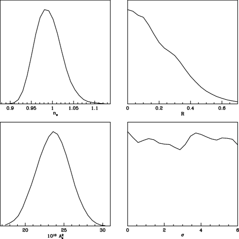
Figure 1: Marginalized probability distributions of inflationary parameters ($n_{s}$, $R$, $A_{s}^{2}$, $\sigma$) for the GR case with prior $0\leq\sigma\leq 6$ and $\epsilon_{3}=0$. The likelihood analysis does not choose a preferred value of the noncommutative parameter $\sigma$.

Since the UV commutative case has already been investigated in literature, we will concentrate ourselves to the IR noncommutative region. This choice is also dictated by a technical reason. In the commutative limit $\sigma$ depends upon both the Hubble parameter, evaluated at the horizon crossing, and the string mass $M_{s}$. As we have seen, even if the tensor spectral index is fixed by Eq. (22), the introduction of the extra degree of freedom $\sigma$ results in a poor constraint on the parameter itself. On the contrary, in the far IR region the function $\sigma$ approaches nonzero constant values as shown in Table 2. This allows us to impose the consistency equation (22) and concretely reduce the space of parameters, setting a meaningful scheme of analysis for the noncommutative models. Moreover, the amplitude of gravitational waves is strongly damped for angular scales with $\ell\gtrsim 10$ and the relations (19) and (22) only affect the large scales with $\ell\lesssim 10$, corresponding to the IR region. In this sense, using a constant $\sigma$ is a good approximation.

In Fig. 2 we plot the $1\sigma$ and $2\sigma$ observational contour bounds for the GR case with $\sigma=0$ (GR0), $\sigma=6$ (GR1) and $\sigma=2$ (GR2). Figures 3 and 4 correspond to the likelihood contours for the RS and GB cases, respectively. These results hold for both the scalar field $\phi$ and the tachyon field $T$ because of the use of the HF parameters.

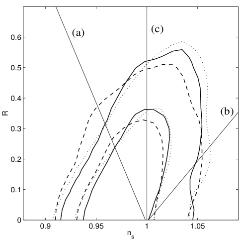
Figure 2: The $1\sigma$ and $2\sigma$ observational contour bounds for the GR case. Each contour curve corresponds to (a) GR0 ($\sigma=0$), solid line; (b) GR1 ($\sigma=6$), dashed line; (c) GR2 ($\sigma=2$), dotted line. We also show the border of large-field and hybrid inflationary models for (a) GR0, (b) GR1 and (c) GR2 cases. The region on the left of each border corresponds to the parameter space in large-field models. Noncommutative spacetime allows the border extending to the region $n_{s}>1$.

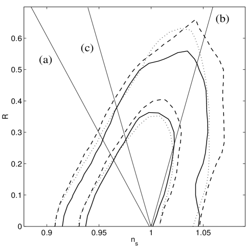
Figure 3: The $1\sigma$ and $2\sigma$ observational contour bounds for the RS case. The meaning of the curves and the borders are the same as in Fig. 2.

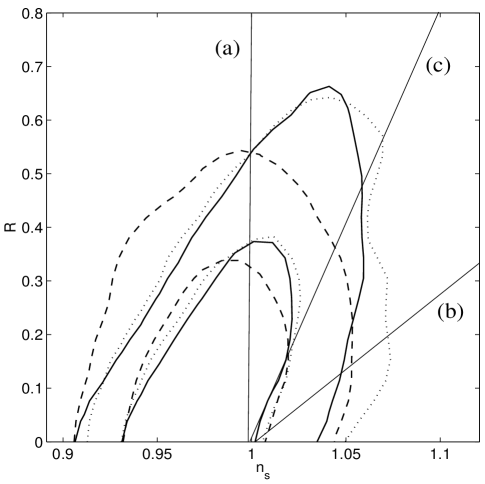
Figure 4: The $1\sigma$ and $2\sigma$ observational contour bounds for the GB case. The meaning of the curves and the borders are the same in Fig. 2.

In the GR case, the class 2 ($\sigma=2$) is rather special since $R$ and $n_{t}$ vanish. The class 2 contour extends to higher values of $R$ relative to the commutative plot, while the class 1 contour allows larger values of $|n_{s}-1|$ but with a smaller $R_{\rm max}$. Thus the noncommutativity of a model is not monotonically measured by $\sigma$ (with greater $\sigma$ corresponding to larger effects) and nonlocal features make their appearance in a nontrivial way.

We can do similar considerations for the RS case (where the maximal elongation is achieved for $\sigma=6$) and for the GB one (where the class 1 behaves in a totally different manner); see Figs. 3 and 4. Note that the degeneracy between GR and RS is removed for $\sigma>0$, both from a theoretical and observational point of view.

IV Theoretical values of inflationary observables in large-field noncommutative models

While the HF equations of Sec. II are independent of the kind of inflaton when expressed via the horizon-flow parameters, the difference appears when we constrain inflationary potentials. This can be clearly understood in the SR formalism, using the potential SR tower $\{\epsilon_{\text{\tiny$\phi V$}},\eta_{\text{\tiny$\phi V$}},\xi_{\text{\tiny$\phi V$}},\dots\}$ described in cal3 , together with the first-order relations $\epsilon_{\text{\tiny$\phi$}}\approx\epsilon_{\text{\tiny$\phi V$}}$, $\eta_{\text{\tiny$\phi$}}\approx\eta_{\text{\tiny$\phi V$}}-\epsilon_{\text{\tiny$\phi V$}}$, $\xi_{\text{\tiny$\phi$}}^{2}\approx\xi_{\text{\tiny$\phi V$}}^{2}-3\epsilon_{\text{\tiny$\phi V$}}\eta_{\text{\tiny$\phi V$}}+(3-\theta)\epsilon_{\text{\tiny$\phi V$}}^{2}$. Even if the dynamical conditions are slightly more precise within the Hubble SR formalism, the potential approximation fits better for our analysis. The inflationary observables $A_{s}^{2}$, $n_{s}$ and $R$ read, to lowest SR order,

$$A_{s}^{2}(\phi) = \frac{9\beta_{q}^{6}}{25\pi^{2}}\frac{V^{3q}}{V^{\prime 2}}\Sigma^{2}\,,$$ (27a)

$$n_{s}-1 = 2\eta_{\text{\tiny$\phi$}}-(4-\sigma)\,\epsilon_{\text{\tiny$\phi$}}$$ (27b)

$$= \frac{1}{3\beta_{q}^{2}V^{q}}\left[2V^{\prime\prime}+(\sigma-6)\frac{q}{2}\frac{V^{\prime 2}}{V}\right]\,,$$ (27c)

$$R = \frac{16q}{6\beta_{q}^{2}\zeta_{q}}\frac{V^{\prime 2}}{V^{q+1}}\,.$$ (27d)

For the tachyon, $\epsilon_{\text{\tiny$T$}}\approx\epsilon_{\text{\tiny$TV$}}$, $\eta_{\text{\tiny$T$}}\approx\eta_{\text{\tiny$TV$}}$, $\xi_{\text{\tiny$T$}}^{2}\approx\xi_{\text{\tiny$TV$}}^{2}+3\epsilon_{\text{\tiny$TV$}}\eta_{\text{\tiny$TV$}}$, and the inflationary observables are

$$A_{s}^{2}(T) = \frac{9\beta_{q}^{6}}{25\pi^{2}}\frac{V^{3q+1}}{V^{\prime 2}}\Sigma^{2}\,,$$ (28a)

$$n_{s}-1 = 2\eta_{\text{\tiny$T$}}-(2+\theta-\sigma)\,\epsilon_{\text{\tiny$T$}}$$ (28b)

$$= \frac{1}{3\beta_{q}^{2}V^{q}}\left[2U^{\prime\prime}-(4+\theta-\sigma)\frac{q}{2}U^{\prime 2}\right]\,,$$ (28c)

$$R = \frac{16q}{6\beta_{q}^{2}\zeta_{q}}\frac{V^{\prime 2}}{V^{q+2}}\,.$$ (28d)

In this and the following section we shall consider an important class of inflaton potentials, namely, the large-field models

$$V(\varphi)=V_{0}\varphi^{p}\,,\qquad\varphi=\phi,\,T\,,$$ (29)

in which the inflaton field starts with a large initial value and rolls down toward the potential minimum at smaller $\varphi$. The linear potential with $p=1$ corresponds to the border of large-field and small-field models. The exponential potential

$$V=V_{0}\exp\left(-\varphi/\varphi_{0}\right)\,,$$ (30)

characterizes the border of large-field and hybrid models. This case can be regarded as the $p\to\infty$ limit of the polynomial potential (29).

Making use of slow-roll approximations $\big{|}\ddot{\phi}\big{|}\ll\big{|}3H\dot{\phi}\big{|}$ and $\dot{\phi}^{2}\ll V(\phi)$, we obtain

$$N(\phi)\approx-3\beta_{q}^{2}\int_{\phi}^{\phi_{f}}\frac{V^{q}}{V^{\prime}}\,d\phi\,,$$ (31)

for the scalar field $\phi$, and

$$N(T)\approx-3\beta_{q}^{2}\int_{T}^{T_{f}}\frac{V^{q+1}}{V^{\prime}}\,dT\,,$$ (32)

for the tachyon field $T$. Here we make use of the backward definition $N=\ln(a_{f}/a)$ of the number of $e$-foldings; see footnote 2.

The potentials (29) and (30) cover a number of exact solutions either exactly or approximately cal3 . In fact, the commutative solutions of Ref. cal3 are perfectly viable in the noncommutative case too, since the nonlocal physics does not affect the homogeneous background. The unique apparently subtle point is that in the IR region one explicitly uses the exponential solution to construct the perturbation amplitudes, contrary to the UV case in which it is implicitly assumed in the approximation of constant SR parameters. However, the subtended philosophy is quite the same, that is to find a general solution with constant nonzero SR parameters and then to perturb it with small time variations. Despite these simple considerations, the predictions of these homogeneous models definitely change when spacetime becomes noncommutative.

IV.1 The ordinary scalar field $\phi$

For the scalar potential (29) with the ordinary scalar field $\phi$, we have

$$n_{s}-1 = -\frac{pV_{0}^{1-q}}{6\beta_{q}^{2}}\frac{p(6q-\sigma q-4)+4}{\phi^{2+(q-1)p}}\,,$$ (33)

$$R = \frac{16qp^{2}}{6\beta_{q}^{2}\zeta_{q}V_{0}^{q-1}}\phi^{(1-q)p-2}\,.$$ (34)

We can estimate the field value at the end of inflation by setting $\epsilon_{\phi}(t_{f})=1$, which yields $\phi_{f}^{p(q-1)+2}\approx qp^{2}/(6\beta_{q}^{2}V_{0}^{q-1})$.

Then the number of $e$-foldings (31) is

$$N=\frac{3\beta_{q}^{2}V_{0}^{q-1}}{p[p(q-1)+2]}\,\phi^{p(q-1)+2}-\frac{qp}{2[p(q-1)+2]}\,,$$ (35)

which is valid for $p\neq 2/(1-q)$. The scalar index and the tensor-to-scalar ratio are

$$n_{s}-1 = -\frac{p(6q-\sigma q-4)+4}{2N(pq-p+2)+pq}\,,$$ (36)

$$R = \frac{16qp}{\zeta_{q}}\frac{1-n_{s}}{p(6q-\sigma q-4)+4}\,.$$ (37)

As discussed in Sec. II, the tensor-to-scalar ratio $R$ does not involve the parameter $\sigma$, since this quantity is invariant by taking the noncommutative effect into account; this is evident when expressing Eq. (37) in terms of $N$. The main change due to spacetime noncommutativity appears for the spectral index $n_{s}$.

For the commutative spacetime ($\sigma=0$) one can easily verify that the above results reduce to what was derived in LS for the GR ($q=1,\zeta_{1}=1$) and RS ($q=2,\zeta_{2}=2/3$) scenarios. In these cases scalar perturbations are red tilted ($n_{s}<1$). The spectrum can be blue tilted when noncommutativity is switched on. For example, let us consider the noncommutative limit $\sigma\to 6$. In this case we have

$$n_{s}-1=\frac{4(p-1)}{2N(pq-p+2)+pq}\qquad\text{for}~{}~{}\sigma\to 6\,,$$ (38)

which means $n_{s}>1$ for $p>1$. Therefore it is possible to explain the loss of power in the spectrum at large scales, as we shall see in the next section.

The exponential potential (30) corresponds to the limit $p\to\infty$ in Eqs. (36) and (37), thereby yielding

$$n_{s}-1 = \frac{4-(6-\sigma)q}{2N(q-1)+q}\,,$$ (39)

$$R = \frac{16q}{\zeta_{q}[2N(q-1)+q]}\,,$$ (40)

which is valid for $q\neq 1$. This gives the border between large-field and hybrid models

$$R=-\frac{16q}{\zeta_{q}(6q-\sigma q-4)}(n_{s}-1)\,.$$ (41)

In the case of GR ($q=1$) we find that the border of large-field and hybrid models extends to the region of $n_{s}>1$ for $\sigma>2$. Thus, in the regime where the noncommutative effect becomes important ($2\leq\sigma\leq 6$), one can obtain a blue-tilted spectrum even in the large-field models, which is not possible in the commutative case.

Note that the border of large-field and small-field models corresponds to $p=1$, giving

$$R=-\frac{16}{\zeta_{q}(6-\sigma)}(n_{s}-1)\,.$$ (42)

This border does not extend to the region $n_{s}>1$ for $\sigma<6$.

IV.2 The tachyon field $T$

For the scalar potential (29) with the tachyon field $T$, we have

$$n_{s}-1 = -\frac{p}{6\beta_{q}^{2}V_{0}^{q}}\frac{pq(4+\theta-\sigma)+4}{T^{2+qp}}\,,$$ (43)

$$R = \frac{16qp^{2}}{6\beta_{q}^{2}\zeta_{q}V_{0}^{q}}T^{-2-qp}\,.$$ (44)

Since inflation ends at $T_{f}^{qp+2}\approx qp^{2}/(6\beta_{q}^{2}V_{0}^{q})$, the number of $e$-foldings is estimated as

$$N=\frac{3\beta_{q}^{2}V_{0}^{q}}{p(pq+2)}\,T^{pq+2}-\frac{qp}{2(pq+2)}\,,\qquad p\neq-\frac{2}{q}\,.$$ (45)

Then we get

$$n_{s}-1 = -\frac{p(6q-\sigma q-2)+4}{2N(pq+2)+pq}\,,$$ (46)

$$R = \frac{16qp}{\zeta_{q}}\frac{1-n_{s}}{p(6q-\sigma q-2)+4}\,,$$ (47)

where we used Eq. (8). For the GR0 spacetime ($q=1$ and $\sigma=0$), these results reproduce what was obtained in Ref. SV . The tensor-to-scalar ratio is smaller relative to the case of the ordinary scalar field $\phi$, thus preferred observationally GST . The effect of noncommutativity can lead to a blue-tilted spectrum ($n_{s}>1$) as is similar to the case of the field $\phi$.

For the exponential potential (30) one gets

$$n_{s}-1 = -\frac{4+\theta-\sigma}{2N+1}\,,$$ (48)

$$R = \frac{16}{\zeta_{q}(2N+1)}\,,$$ (49)

which is obtained by taking the limit $p\to\infty$ in Eqs. (46) and (47). This gives the border of large-/hybrid-field models

$$R=-\frac{16}{\zeta_{q}(4+\theta-\sigma)}(n_{s}-1)\,.$$ (50)

In the GR case this border belongs to the region $n_{s}>1$ for $\sigma>4$.

The border of large-/small-field models is

$$R=-\frac{16q}{\zeta_{q}(6q-\sigma q+2)}(n_{s}-1)\,,$$ (51)

which does not extend to the region $n_{s}>1$ for $\sigma<6$.

IV.3 The difference between $\phi$ and $T$

By Eqs. (36) and (46) we find that the difference between the ordinary field and the tachyon field for the spectral index $n_{s}$ appears both in the denominator and the numerator. Meanwhile by Eqs. (37) and (47) the difference for the ratio $R$ only appears in the denominator

$$R=\frac{16qp}{\zeta_{q}[2N(qp+2-b)+qp]}\,,$$ (52)

where $b=p$ for $\varphi=\phi$ and $b=0$ for $\varphi=T$. Therefore the tensor-to-scalar ratio in the tachyon case is smaller than in the ordinary scalar field case when $p>0$. This property implies that the tachyon inflation is less affected by an observational pressure as was pointed out in the GR commutative case GST . In the next section we shall study this issue in detail in the context of noncommutative inflation.

V Observational constraints on large-field noncommutative models

In this section we place constraints on large-field noncommutative inflationary models using the observational contour bounds obtained in Sec. III. We plot the theoretical values of $n_{s}$ and $R$ for $N=45,50,55,60$ on the likelihood contours. Typically one can restrict the number of $e$-folds to $N\lesssim 65$ LL2 , but it is sufficient to show the values up to $N=60$ to judge whether the models we consider are ruled out or not.

Before considering each noncommutative case, it is important to understand the basic structure of the theoretical curves on the $n_{s}$-$R$ plane. The effect of the noncommutative parameter $\sigma$ has a straightforward geometrical interpretation. Let us define $x\equiv n_{s}-1$ and $y\equiv R$, together with the polar coordinates $\varrho\equiv\sqrt{x^{2}+y^{2}}$ and $\sin\vartheta\equiv y/\varrho$ centered at $(1,0)$ in the $n_{s}$-$R$ plane. From the last section, we know that

$$y = \gamma(q,p,\sigma)x\,,$$ (53)

$$\gamma(q,p,\sigma) = -\frac{16qp}{\zeta_{q}[p(6q-\sigma q-c)+4]}\,,$$ (54)

where $c=4$ for $\varphi=\phi$ and $c=2$ for $\varphi=T$. Then, $\varrho^{2}=(1+\gamma^{2})x^{2}$ and $\tan\vartheta=\gamma$. Since $pq>0$ in the cases we consider, $\vartheta$ is a decreasing function in terms of $\sigma$. Therefore, as $\sigma$ increases, the theoretical points are rotated clockwise in the $\varrho$-$\vartheta$ plane. This rotation is mainly governed by $\sigma$ rather than $p$ when $p$ is large, which can be seen from the computation of the logarithmic variation of $\gamma$:

$$\frac{d\ln\gamma}{dp}=\frac{4}{qp^{2}}\frac{d\ln\gamma}{d\sigma}\,.$$ (55)

This also implies that, for a given $\sigma$, the three models $p=2,4,+\infty$ lie on a wider range of radii for smaller values of $q$. As we shall see later, this effect is particularly evident in the Gauss-Bonnet case with respect to the GR and RS cases in the same (non)commutative class.

The divergence of $\gamma$ at the asymptote $\vartheta=\pi/2$ identifies those models generating a scale-invariant scalar spectrum $n_{s}=1$. They are listed in Table 3 for fixed $\sigma$ and $q$. In particular, ordinary scalar class 2 models cannot give $n_{s}=1$ if one imposes the condition $p(q-1)+2\neq 0$ for inflation to have a natural end. The tachyonic counterparts are those with $pq+2\neq 0$, and only the GR2 case is excluded.

Note that class 1 patch models admit only one scale-invariant potential for each inflaton, that is, the linear potential for $\phi$ and the quadratic one for $T$. Another frequent case is $p=-2$ (scalar GR0, tachyon GR2 and tachyon GB2), which however does not match with the exact power-law solutions of cal3 (RS scalar and GR tachyon). Anyway our interest in this paper are the models with positive $p$ ($p\geq 2$) that lead to natural reheating.

Table 3: Values of $p$ for scale-invariant models.

		$\sigma$
		0 (Class 0)	6 (Class 1)	2 (Class 2)
	GR	$-2$	1	$\infty$
$\phi$	RS	$-1/2$	1	$-1$
	GB	$\infty$	1	3
	GR	$-1$	2	$-2$
$T$	RS	$-2/5$	2	$-2/3$
	GB	$-2$	2	$-6$

V.1 The ordinary scalar field $\phi$

Let us first study the observational constraints on the large-field models for the ordinary field $\phi$. In Figs. 5–7 the theoretical values (36) and (37) for the potential (29) are plotted in the GR, RS, and GB cases together with $1\sigma$ and $2\sigma$ contour bounds. Hereafter we shall consider each case separately in order to clarify the situation.

V.1.1 GR case

It is well known that the commutative GR case ($\sigma=0$) is observationally disfavoured for the quartic potential ($p=4$). In this case the theoretical points are outside of the $2\sigma$ contour bound for a number of $e$-folds $N<60$.

In the noncommutative class 1 case ($\sigma=6$) the spectral index $n_{s}$ is larger than 1 by Eq. (38). The tensor-to-scalar ratio $R$ is independent of $\sigma$, so this value is the same as the one in the class 0. As one can see in Fig. 5 the quartic potential is outside of the $2\sigma$ bound for $N<55$. Therefore this case is also marginal as in the class 0 case.

The noncommutative class 2 case ($\sigma=2$) corresponds to a scalar spectral index smaller than 1, but it is closer to a scale-invariant spectrum relative to the class 0 case. This shifts the theoretical points inside of the $2\sigma$ bound and allows the quartic potential even for $N=45$. Then a “mild” spacetime noncommutativity in which $\sigma$ is close to 2 is favoured for the observational compatibility of the quartic potential. Note that the quadratic potential ($p=2$) is allowed in all three models, irrespective of the degree of noncommutativity, as clearly shown in Fig. 5.

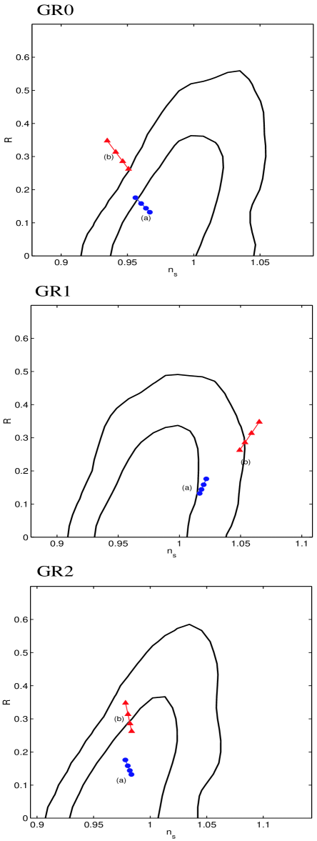
Figure 5: Observational constraints on large-field models for the GR ordinary field $\phi$ together with the $1\sigma$ and $2\sigma$ contour bounds for three classes of commutative/noncommutative scenarios. The theoretical values correspond to (a) $p=2$ (dots) and (b) $p=4$ (triangles), respectively, with the number of $e$-folds $N=45,50,55,60$ (from top to bottom).

V.1.2 RS case

In commutative RS spacetime, the quartic potential is under a strong observational pressure as is similar to the GR0 case, and the steep inflation driven by an exponential potential ($p\to\infty$) is ruled out LS ; TL .

This situation is improved in the class 1 noncommutative scenario. Since the spectral index $n_{s}$ takes a value which is slightly larger than 1 and the $2\sigma$ contour bounds extend to the region with $R>0.6$, even the steep inflation is allowed (see Fig. 6).

Meanwhile in the class 2 case the exponential potential is outside of the $2\sigma$ bound unless the number of $e$-folds $N$ is larger than 60. The quartic potential moves inside of the $2\sigma$ bound relative to the class 0 case, thus becoming compatible with observations.

In the RS case strong noncommutativity close to $\sigma=6$ is favoured observationally rather than mild noncommutativity like $\sigma=2$, in contrast with the GR case.

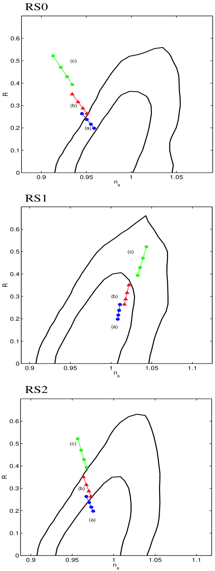
Figure 6: Observational constraints on large-field models for the RS ordinary field $\phi$. Each case corresponds to (a) $p=2$ (dots), (b) $p=4$ (triangles) and (c) exponential potential with $p\to\infty$ (squares), respectively, with the number of $e$-folds $N=45,50,55,60$ (from top to bottom).

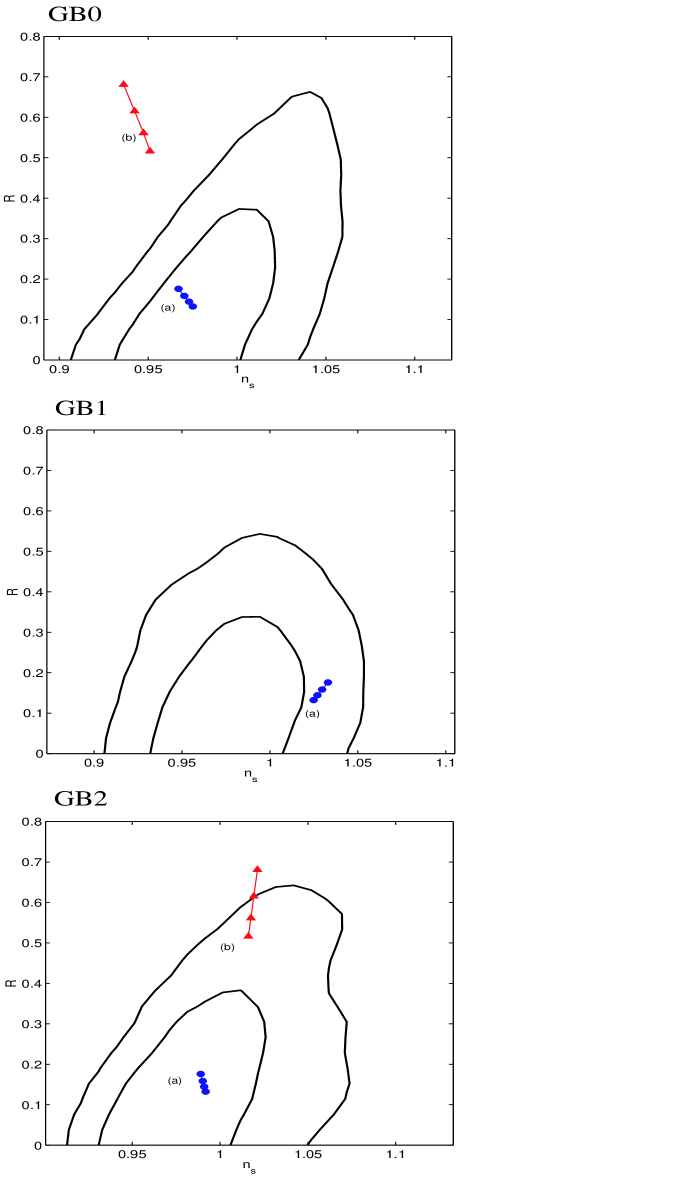
Figure 7: Observational constraints on large-field models for the GB ordinary field $\phi$. Each case corresponds to (a) $p=2$ (dots) and (b) $p=4$ (triangles), respectively, with the number of $e$-folds $N=45,50,55,60$ (from top to bottom). In the GB1 case the quadratic potential is far outside of the $2\sigma$ bound.

V.1.3 GB case

In the Gauss-Bonnet braneworld cosmology the GB dominant stage with $q=2/3$ is followed by the RS stage with $q=2$. In Ref. TSM theoretical values of $n_{s}$ and $R$ were derived for the case where inflation ends in the RS regime. In this work we study a situation in which the end of inflation corresponds to the GB regime. In this case we do not have a sufficient amount of $e$-folds for $p>6$, so it is not meaningful to consider steep inflation.

In commutative spacetime the quartic potential is ruled out observationally, while the quadratic potential is inside of the $1\sigma$ bound, see Fig. 7.

In the class 1 case the spectral index for the quartic model is larger than 1.1 for a number of $e$-folds $N<65$, thus far outside of the $2\sigma$ bound. In this sense the effect of strong noncommutativity close to $\sigma=6$ is not welcome to save the quartic potential. On the other hand, the quadratic potential is not ruled out due to a little departure from scale invariance.

The class 2 noncommutative scenario exhibits an interesting feature to have $n_{s}$ close to 1 even for the quartic potential. As seen in Fig. 7 the quartic potential is within the $2\sigma$ bound for $N>50$, thereby compatible with observations. This situation is similar to the GR case.

V.2 The tachyon field $T$

Let us next consider the observational constraint on the tachyonic large-field models.

V.2.1 GR case

The GR commutative case was already investigated in Refs. SV ; GST . Since the tensor-to-scalar ratio is smaller relative to the normal scalar field case, this leads to the compatibility with observations. Even steep inflation is deep within the $2\sigma$ contour bound.

Because of this small value of $R$, the class 1 and class 2 noncommutative scenarios are also allowed as shown in Fig. 8. The class 1 scenario corresponds to a spectral index $n_{s}$ larger than 1, but this does not deviate from a scale-invariant spectrum. All cases with $p=2$, $p=4$ and $p=\infty$ are inside of the $2\sigma$ contour bound.

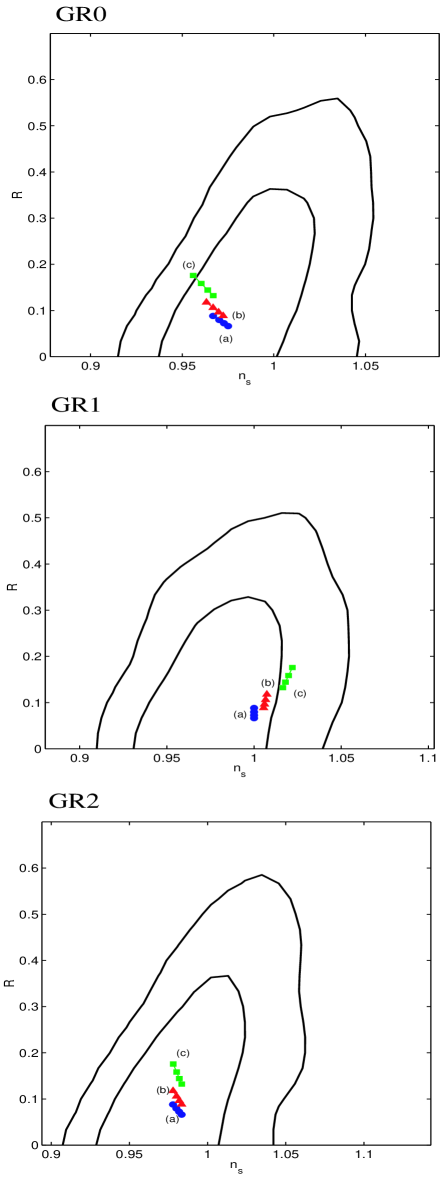
Figure 8: Observational constraints on large-field models for the GR tachyon field $T$ together with the $1\sigma$ and $2\sigma$ contour bounds for three classes of commutative/noncommutative scenarios. Each case corresponds to (a) $p=2$ (dots), (b) $p=4$ (triangles) and (c) exponential potential with $p\to\infty$ (squares), respectively, with the number of $e$-folds $N=45,50,55,60$ (from top to bottom).

V.2.2 RS case

The RS case exhibits larger values of the tensor-to-scalar ratio compared to the GR case. However, the quadratic and quartic potentials are always within the $2\sigma$ bound. The exponential potential is also allowed for the $e$-folds with $N\gtrsim 50$. See Fig. 9.

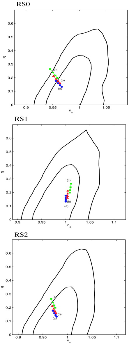
Figure 9: Observational constraints on large-field models for the RS tachyon field $T$. Each case corresponds to (a) $p=2$ (dots), (b) $p=4$ (triangles) and (c) exponential potential with $p\to\infty$ (squares), respectively, with the number of $e$-folds $N=45,50,55,60$ (from top to bottom).

V.2.3 GB case

By Eq. (55) each inflationary model ($p=2,4,\infty$) in the GB case ($q=2/3$) lies on a wider range of radii $\varrho$ relative to the GR and RS cases. In spite of this property, even steep inflation is compatible with observations in both commutative and noncommutative spacetimes. In summary, tachyon inflation is allowed irrespective of the slope of the potential due to a small tensor-to-scalar ratio in all patch cosmologies we have considered. See Fig. 10.

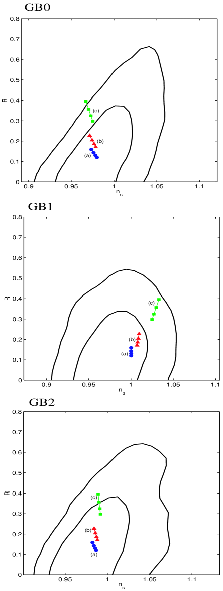
Figure 10: Observational constraints on large-field models for the GB tachyon field $T$. Each case corresponds to (a) $p=2$ (dots), (b) $p=4$ (triangles) and (c) exponential potential with $p\to\infty$ (squares), respectively, with the number of $e$-folds $N=45,50,55,60$ (from top to bottom).

V.3 Suppression of CMB low multipoles in noncommutative inflation

In Refs. HL1 ; TMB ; HL2 it was shown that it is possible to explain the loss of the power spectrum at low multipoles at least partially using the modified spectrum in the UV regime ($\tau\gg kl_{s}^{2}$). Here we will consider the situation in which the spectrum on cosmologically relevant scales is generated in the IR noncommutative regime.

As seen in the likelihood contours, the best-fit value of $n_{s}$ is smaller than 1 and is insensitive to which prescription we adopt for the spacetime (non)commutative structure. The loss of power on largest scales is difficult to be explained in the standard concordance scenario. If we take the effect of spacetime noncommutativity into account, it is possible to have a suppression of power due to a blue-tilted spectrum. For example, the potential (29) gives rise to the blue spectrum for the GR1 noncommutative case. Of course, the large spectral index $n_{s}\gtrsim 1.05$ is ruled out as seen in Fig. 5, but the quadratic potential ($p=2$) gives the observationally allowed value around $n_{s}\sim 1.02$. The quartic potential ($p=4$) corresponds to a marginal compatibility with observations, but it is welcome to explain the loss of power on the largest scales.

In Fig. 11 we plot the CMB angular power spectra for several different cases. The spectrum exhibits some suppression around $1<l\lesssim 10$ in noncommutative spacetime relative to the commutative one. The quartic potential leads to a stronger suppression compared to the quadratic one, but the smaller-scale spectrum tends to show some disagreement with observations for larger $n_{s}$. Anyway, it is intriguing that single-field noncommutative inflation leads to a blue-tilted spectrum suitable for explaining the loss of power at low multipoles, since this is difficult to be achieved in commutative spacetime unless we introduce another scalar field as in the case of hybrid inflation (see also LMMR ).

Figure 11: The CMB angular power spectrum showing the effects of suppression of power at low multipoles. Curve (a) is the GR commutative model with $(n_{s},R)=(0.967,0.132)$ corresponding to the quadratic potential. Curves (b) and (c) are the GR1 noncommutative scenario with $(n_{s},R)=(1.018,0.144)$ and $(n_{s},R)=(1.049,0.263)$, respectively. Note that these values are achieved for the quadratic and quartic potentials in the GR1 case, respectively.

VI Conclusion and discussion

In this paper we have investigated observational constraints on a number of patch noncommutative inflationary scenarios including general relativity, Randall-Sundrum and Gauss-Bonnet braneworld. We expressed the inflationary observables {$A_{s}^{2}$, $R$, $n_{s}$, $n_{t}$, $\alpha_{s}$, $\alpha_{t}$} in terms of horizon-flow parameters both for a normal scalar field $\phi$ and a tachyon field $T$. We showed that the likelihood analysis of the observables is the same for both types of scalar fields by using HF parameters. It is known that the consistency relation between the tensor spectral index and the tensor-to-scalar ratio is the same both in commutative GR and RS cases. This property also holds in induced-gravity braneworld inflation BMW and in generalized Einstein theories including four-dimensional dilaton gravity and scalar-tensor theories TG04 . The spacetime noncommutativity breaks this degeneracy and provides a variety of consistency relations [see Eq. (22) and Table 2]. We have considered two classes of noncommutative models and evaluated the power spectra in the IR limit. The strength of noncommutativity is measured by a parameter $\sigma$, and we classified the models into three classes: (i) commutative spacetime with $\sigma=0$, (ii) the class 1 IR case with $\sigma=6$ and (iii) the class 2 IR case with $\sigma=2$. The perturbations are always blue-tilted for the class 1 scenario, thus giving positive values of $n_{t}/R$. This unusual property comes from the fact that the mechanism for generating fluctuations is different from the standard case due to the existence of the stringy uncertainty relation.

We carried out likelihood analyses in terms of inflationary and cosmological parameters using the data set coming from WMAP, the 2dF, and SDSS galaxy redshift surveys. The numerical analysis showed that both the HF parameter $\epsilon_{3}$ and the slow-roll parameter $\xi^{2}$ are poorly constrained and can be consistently set equal to zero. We ran the code by varying the parameter $\sigma$ in the range $0\leq\sigma\leq 6$ and found that $\sigma$ does not show a good convergence. This means that current observations do not choose a preferred commutative or noncommutative model. We then performed a likelihood analysis for three fixed values of $\sigma$ ($\sigma=0,2,6$). As seen in Figs. 2–4 one can find some difference in the $n_{s}$-$R$ plane by the modification of consistency relations due to noncommutative spacetime. The main change appears in the maximum value of $R$ ($=R_{\text{max}}$) and it ranges in the region $0.5\lesssim R_{\text{max}}\lesssim 0.7$.

We also placed constraints on the large-field monomial potential (29) for noncommutative GR/RS/GB scenarios. We found the following interesting results.

For the ordinary scalar field $\phi$:

• The quartic potential is rescued from the marginal rejection in the noncommutative class 2 GR case ($\sigma=2$).

• Steep inflation driven by an exponential potential is allowed in the noncommutative class 1 RS case ($\sigma=6$). The quartic potential is compatible with observations both in the class 1 and class 2 RS cases, but it is not so in the RS commutative case.

• The quartic potential exhibits a compatibility with observations for the class 2 GB case, while it does not in the other two cases (GB0 and GB1).

For the tachyon field $T$:

• A scale-invariant spectrum ($n_{s}=1$) is generated for $p=2$ in the noncommutative class 1 case irrespective of the kind of patch cosmologies.

• Even steep inflation is allowed due to small values of the tensor-to-scalar ratio in three classes of patch cosmologies.

All these properties have been investigated both analytically and numerically. We also pointed out the possibility to explain the suppression of CMB low multipoles using a blue-tilted spectrum generated in the IR regime of noncommutative spacetime. Note that this is different from the approach in Ref. TMB in which an intermediate spectrum between the IR and UV regions is used to explain the loss of power. Although noncommutativity can provide a better fit of the spectrum for low multipoles, it is not easy to explain the loss of power at $\ell=2,3$. The suppression in this region, corresponding to the Sachs-Wolfe plateau, is difficult to be achieved even with a very blue-tilted spectrum $n_{s}\gtrsim 3$ PTZ especially for $\ell=2$. This is still an open issue and would deserve further study.

It would be interesting to investigate whether some regions of the line of patches $\theta$ are excluded or not by observations. A clear answer in this respect would constrain any new braneworld scenario with a nonstandard Friedmann equation with $\theta\neq 0,\pm 1$. In the GR case ($\theta=0$), we have addressed a similar question for $\sigma$ and performed a likelihood analysis with a very large prior ($|\sigma|<100$). The parameter did not show a good convergence, since the tensor index $n_{t}$ can be made smaller by choosing a smaller $R$ in Eq. (22). Since the same result holds when varying the set $\{\theta,n_{t},\zeta_{q}R\}$, one has to consider fixed values of any extra parameter which modifies the four-dimensional scenario. Then we cannot say anything a priori about the viability of a general patch cosmology.

A fundamental question to be answered is: What about cosmic confusion? Can we rely on the consistency equations as a smoking gun for both braneworld and noncommutative scenarios? The answer is presumably no, since, as it typically happens in cosmology, other completely different frameworks could mimic the features we have exploited. With this sky tolerance, even simple 4D multifield configurations produce a nonstandard set of consistency relations (See Refs. BMR ; WBMR ; TPB ). The subject has to be further explored in a more precise way than that provided by the patch formalism in order to find out more characteristic and sophisticated predictions.

References

- (1) C.L. Bennett et al., Astrophys. J., Suppl. Ser. 148, 1 (2003) [arXiv:astro-ph/0302207].
- (2) D.N. Spergel et al., Astrophys. J., Suppl. Ser. 148, 175 (2003) [arXiv:astro-ph/0302209].
- (3) H.V. Peiris et al., Astrophys. J., Suppl. Ser. 148, 213 (2003) [arXiv:astro-ph/0302225].
- (4) S.L. Bridle, A.M. Lewis, J. Weller, and G. Efstathiou, Mon. Not. R. Astron. Soc. 342, L72 (2003) [arXiv:astro-ph/0302306].
- (5) V. Barger, H.S. Lee, and D. Marfatia, Phys. Lett. B 565, 33 (2003) [arXiv:hep-ph/0302150].
- (6) W.H. Kinney, E.W. Kolb, A. Melchiorri, and A. Riotto, Phys. Rev. D 69, 103516 (2004) [arXiv:hep-ph/0305130].
- (7) S.M. Leach and A.R. Liddle, Phys. Rev. D 68, 123508 (2003) [arXiv:astro-ph/0306305].
- (8) SDSS collaboration, M. Tegmark et al., Phys. Rev. D 69, 103501 (2004) [arXiv:astro-ph/0310723].
- (9) http://astro.estec.esa.nl/SA-general/Projects/Planck/
- (10) L. Randall and R. Sundrum, Phys. Rev. Lett. 83, 4690 (1999) [arXiv:hep-th/9906064].
- (11) R. Maartens, Living Rev. Relativity 7, 1 [arXiv:gr-qc/0312059].
- (12) P. Brax, C. van de Bruck, and A.-C. Davis, arXiv:hep-th/0404011.
- (13) G. Calcagni, Phys. Rev. D 69, 103508 (2004) [arXiv:hep-ph/0402126].
- (14) R. Maartens, D. Wands, B.A. Bassett, and I.P.C. Heard, Phys. Rev. D 62, 041301 (2000) [arXiv:hep-ph/9912464].
- (15) D. Langlois, R. Maartens, and D. Wands, Phys. Lett. B 489, 259 (2000) [arXiv:hep-th/0006007].
- (16) G. Huey and J.E. Lidsey, Phys. Lett. B 514, 217 (2001) [arXiv:astro-ph/0104006].
- (17) G. Huey and J.E. Lidsey, Phys. Rev. D 66, 043514 (2002) [arXiv:astro-ph/0205236].
- (18) A.R. Liddle and A.J. Smith, Phys. Rev. D 68, 061301 (2003) [arXiv:astro-ph/0307017].
- (19) S. Tsujikawa and A.R. Liddle, J. Cosmol. Astropart. Phys. 03, 001 (2004) [arXiv:astro-ph/0312162].
- (20) J.E. Lidsey and N.J. Nunes, Phys. Rev. D 67, 103510 (2003) [arXiv:astro-ph/0303168].
- (21) J.F. Dufaux, J.E. Lidsey, R. Maartens, and M. Sami, Phys. Rev. D 70, 083525 (2004) [arXiv:hep-th/0404161].
- (22) S. Tsujikawa, M. Sami, and R. Maartens, Phys. Rev. D 70, 063525 (2004) [arXiv:astro-ph/0406078].
- (23) S. Alexander, R. Brandenberger, and J. Magueijo, Phys. Rev. D 67, 081301 (2003) [arXiv:hep-th/0108190].
- (24) R. Brandenberger and P.-M. Ho, Phys. Rev. D 66, 023517 (2002) [arXiv:hep-th/0203119].
- (25) Q.-G. Huang and M. Li, J. High Energy Phys. 06, 014 (2003) [arXiv:hep-th/0304203].
- (26) M. Fukuma, Y. Kono, and A. Miwa, Nucl. Phys. B682, 377 (2004) [arXiv:hep-th/0307029].
- (27) M. Fukuma, Y. Kono, and A. Miwa, eprint arXiv:hep-th/0312298.
- (28) S. Tsujikawa, R. Maartens, and R. Brandenberger, Phys. Lett. B 574, 141 (2003) [arXiv:astro-ph/0308169].
- (29) Q.-G. Huang and M. Li, J. Cosmol. Astropart. Phys. 11, 001 (2003) [arXiv:astro-ph/0308458].
- (30) Q.-G. Huang and M. Li, arXiv:astro-ph/0311378.
- (31) D.-J. Liu and X.-Z. Li, arXiv:astro-ph/0402063.
- (32) H.S. Kim, G.S. Lee, and Y.S. Myung, arXiv:hep-th/0402018.
- (33) H.S. Kim, G.S. Lee, H.W. Lee, and Y.S. Myung, arXiv:hep-th/0402198.
- (34) R.-G. Cai, Phys. Lett. B 593, 1 (2004) [arXiv:hep-th/0403134].
- (35) F. Lizzi, G. Mangano, G. Miele, and M. Peloso, J. High Energy Phys. 06, 049 (2002) [arXiv:hep-th/0203099].
- (36) S.A. Alavi and F. Nasseri, arXiv:astro-ph/0406477.
- (37) G. Calcagni, Phys. Rev. D to appear [arXiv:hep-th/0406006].
- (38) G. Calcagni, arXiv:hep-ph/0406057.
- (39) Y.S. Myung, arXiv:hep-th/0407066.
- (40) K.H. Kim and Y.S. Myung, arXiv:astro-ph/0406387.
- (41) G.W. Gibbons, Phys. Lett. B 537, 1 (2002) [arXiv:hep-th/0204008].
- (42) D. Choudhury, D. Ghoshal, D.P. Jatkar, and S. Panda, Phys. Lett. B 544, 231 (2002) [arXiv:hep-th/0204204].
- (43) L. Kofman and A.D. Linde, J. High Energy Phys. 07, 004 (2002) [arXiv:hep-th/0205121].
- (44) M. Sami, P. Chingangbam, and T. Qureshi, Phys. Rev. D 66, 043530 (2002) [arXiv:hep-th/0205179].
- (45) A. Frolov, L. Kofman, and A. Starobinsky, Phys. Lett. B 545, 8 (2002) [arXiv:hep-th/0204187].
- (46) M.C. Bento, O. Bertolami, and A.A. Sen, Phys. Rev. D 67, 063511 (2003) [arXiv:hep-th/0208124].
- (47) M.C. Bento, N.M.C. Santos, and A.A. Sen, arXiv:astro-ph/0307292.
- (48) B.C. Paul and M. Sami, Physical Review D to appear, arXiv:hep-th/0312081.
- (49) J. Raeymaekers, arXiv:hep-th/0406195.
- (50) Y.-S. Piao, R.-G. Cai, X. Zhang, and Y.-Z. Zhang, Phys. Rev. D 66, 121301(R) (2002) [arXiv:hep-ph/0207143].
- (51) M.R. Garousi, M. Sami, and S. Tsujikawa, Phys. Rev. D 70, 043536 (2004) [arXiv:hep-th/0402075].
- (52) S. Kachru, R. Kallosh, A. Linde, and S.P. Trivedi, Phys. Rev. D 68, 046005 (2003) [arXiv:hep-th/0301240].
- (53) D.J. Schwarz, C.A. Terrero-Escalante, and A.A. García, Phys. Lett. B 517, 243 (2001) [arXiv:astro-ph/0106020].
- (54) W.H. Kinney, Phys. Rev. D 66, 083508 (2002) [arXiv:astro-ph/0206032].
- (55) A. Lewis, A. Challinor, and A. Lasenby, Astrophys. J. 538, 473 (2000) [arXiv:astro-ph/9911177].
- (56) A. Lewis and S. Bridle, Phys. Rev. D 66, 103511 (2002) [arXiv:astro-ph/0205436].
- (57) http://camb.info/
- (58) http://lambda.gsfc.nasa.gov/
- (59) W.J. Percival et al., Mon. Not. R. Astron. Soc. 327, 1297 (2001) [arXiv:astro-ph/0105252].
- (60) T.J. Pearson et al., Astrophys. J. 591, 556 (2003) [arXiv:astro-ph/0205388].
- (61) K. Grainge et al., Mon. Not. R. Astron. Soc. 341, L23 (2003) [arXiv:astro-ph/0212495].
- (62) C.L. Kuo et al., Astrophys. J. 600, 32 (2004) [arXiv:astro-ph/0212289].
- (63) D.A. Steer and F. Vernizzi, Phys. Rev. D 70, 043527 (2004) [arXiv:hep-th/0310139].
- (64) A.R. Liddle and S.M. Leach, Phys. Rev. D 68, 103503 (2003) [arXiv:astro-ph/0305263].
- (65) M. Liguori, S. Matarrese, M. Musso, and A. Riotto, arXiv:astro-ph/0405544.
- (66) M. Bouhmadi-López, R. Maartens, and D. Wands, arXiv:hep-th/0407162.
- (67) S. Tsujikawa and B. Gumjudpai, Phys. Rev. D 69, 123523 (2004) [arXiv:astro-ph/0402185].
- (68) Y.-S. Piao, S. Tsujikawa, and X. Zhang, Class. Quantum Grav. 21, 4455 (2004) [arXiv:hep-th/0312139].
- (69) N. Bartolo, S. Matarrese, and A. Riotto, Phys. Rev. D 64, 123504 (2001) [arXiv:astro-ph/0107502].
- (70) D. Wands, N. Bartolo, S. Matarrese, and A. Riotto, Phys. Rev. D 66, 043520 (2002) [arXiv:astro-ph/0205253].
- (71) S. Tsujikawa, D. Parkinson, and B.A. Bassett, Phys. Rev. D 67, 083516 (2003) [arXiv:astro-ph/0210322].