Reverberation mapping of active galactic nuclei

Abstract

Reverberation mapping is a proven technique that is used to measure the size of the broad emission-line region and central black hole mass in active galactic nuclei. More ambitious reverberation mapping programs that are well within the capabilities of Hubble Space Telescope could allow us to determine the nature and flow of line-emitting gas in active nuclei and to assess accurately the systematic uncertainties in reverberation-based black hole mass measurements.

1 Introduction: The Inner Structure of AGNs

There is now general consensus that the long-standing paradigm for active galactic nuclei (AGNs) is basically correct, i.e., that AGNs are fundamentally powered by gravitational accretion onto supermassive collapsed objects. Details of the inner structure of AGNs, however, remain sketchy, although both emission lines and absorption lines reveal the presence of large-scale gas flows on scales of hundreds to thousands of gravitational radii. The accretion disk produces a time-variable high-energy continuum that ionizes and heats this nuclear gas, and the broad emission-line fluxes respond to the changes in the illuminating flux from the continuum source. The geometry and kinematics of the broad-line region (BLR), and fundamentally its role in the accretion process, are not understood. Immediate prospects for understanding this key element of AGN structure do not seem especially promising with the realization that the angular size of the nuclear regions projects to only microarcsecond scales even in the case of the nearest AGNs. Unfortunately, there is only very limited information about the BLR from the emission-line profiles alone, since many simple kinematic models are highly degenerate. Nevertheless, it has been possible to draw a few basic interferences about the nature of the BLR:

1. There is strong evidence for a disk component in at least some AGNs. In particular, there is a relatively small subset of AGNs whose spectra show double-peaked Balmer-line profiles. Double-peaked profiles are generally associated with rotating Keplerian disks.

2. There is strong evidence for an outflowing component in many AGNs. Some emission lines have strong blueward asymmetries, suggesting that we preferentially observe outflowing material on the nearer side of an AGN. Slightly blueshifted (relative to the systemic redshift of the host galaxy) absorption features are quite common in AGNs, and there is a good deal of evidence that this absorption, seen primarily in ultraviolet and X-ray spectra, arises on scales similar to that of the broad emission lines.

3. There is strong evidence that gravitational acceleration by the central source is important. As discussed below, a physical scale for the size of the line-emitting region can be obtained by the process of reverberation mapping. The derived scale length for each line is different, with lines that are characteristic of high-ionization gas arising closer to the central source than lines that are more characteristic of low-ionization gas, thus demonstrating ionization stratification within the BLR. Moreover, the higher ionization lines are broader, and indeed the relationship between size and velocity dispersion of the line-emitting region shows a virial-like relationship, i.e., $r\propto\Delta V^{-2}$, where $r$ is the characteristic scale for a line which has Doppler width $\Delta V$.

The conclusion that gravity is important leads us directly to an estimate of the black hole mass, which we take to be

$$M_{\rm BH}=\frac{fr\Delta V^{2}}{G},$$ (1)

where $G$ is the gravitational constant and $f$ is a scaling factor of order unity that depends on the presently unknown geometry and kinematics of the BLR.

In this brief introduction, we already see the two major reasons that understanding the BLR is of critical importance to understanding the entire quasar phenomenon: (1) we need to understand how the accretion/outflow processes work in AGNs and (2) we need to understand the geometry and kinematics of the BLR to assess possible systematic uncertainties in AGN black-hole mass measurements.

2 Reverberation Mapping Basics

Simply put, the idea behind reverberation mapping is to learn about the structure and kinematics of the BLR by observing the detailed response of the broad emission lines to changes in the continuum. The basic assumptions needed are few and straightforward, and can largely be justified after the fact:

1. The continuum originates in a single central source. The size of the accretion disk in a typical bright Seyfert galaxy is expected to be of order $10^{13}$– $10^{14}$ cm, or about a factor of 100 or so smaller than the BLR turns out to be. It is worth noting that we do not necessarily have to assume that the continuum is emitted isotropically.

2. Light-travel time $\tau_{\rm LT}=r/c$ is the most important time scale. The other potentially important time scales include:

   • The recombination time scale $\tau_{\rm rec}=(n_{e}\alpha_{\rm B})^{-1}$, which is the time for emission-line gas to re-establish photoionization equilibrium in response to a change in the continuum brightness. For typical BLR densities, $n_{e}\approx 10^{10}\,{\rm cm}^{-3}$, $\tau_{\rm rec}\approx 0.1$ hr, i.e., virtually instantaneous relative to the light-travel timescales of days to weeks for luminous Seyfert galaxies.

   • The dynamical time scale for the BLR gas, $\tau_{\rm dyn}\approx r/\Delta V$. For typical luminous Seyferts, this works out to be of order 3–5 years. Reverberation experiments must be kept short relative to the dynamical timescale to avoid smearing the light travel-time effects.

3. There is a simple, though not necessarily linear, relationship between the observed continuum and the ionizing continuum. In particular, the observed continuum must vary in phase with the ionizing continuum, which is what is driving the line variations. This is probably the most fragile of these assumptions since there is some evidence that long-wavelength continuum variations follow those at shorter wavelengths, but the timescales involved are still significantly shorter than the timescales for emission-line response.

Given these assumptions, a linearized response model can be written as

$$\Delta L(V,t)=\int\Psi(V,\tau)\Delta C(t-\tau)\,d\tau,$$ (2)

where $\Delta C(t)$ is the continuum light curve relative to its mean value $\overline{C}$, i.e., $\Delta C(t)=C(t)-\overline{C}$, and, $\Delta L(V,t)$ is the emission-line light curve as a function of line-of-sight Doppler velocity $V$ relative to its mean value $\overline{L}(V)$. The function $\Psi(V,\tau)$ is the “velocity-delay map,” i.e., the BLR responsivity mapped into line-of-sight velocity/time-delay space. It is also sometimes referred to as the “transfer function” and eq. (1) is called the transfer equation. Inspection of this formula shows that the velocity-delay map is essentially the observed response to a delta-function continuum outburst. This makes it easy to construct model velocity-delay maps from first principles.

Consider first what an observer at the central source would see in response to a delta-function (instantaneous) outburst. Photons from the outburst will travel out to some distance $r$ where they will be intercepted and absorbed by BLR clouds and produce emission-line photons in response. Some of the emission-line photons will travel back to the central source, reaching it after a time delay $\tau=2r/c$. Thus a spherical surface at distance $r$ defines an “isodelay surface” since all emission-line photons produced on this surface are observed to have the same time delay relative to the continuum outburst. For an observer at any other location, the isodelay surface would be the locus of points for which the travel from the common initial point (the continuum source) to the observer is constant. It is obvious that such a locus is an ellipsoid. When the observer is moved to infinity, the isodelay surface becomes a paraboloid. We show a typical isodelay surface for this geometry in the top panel of Figure 1.

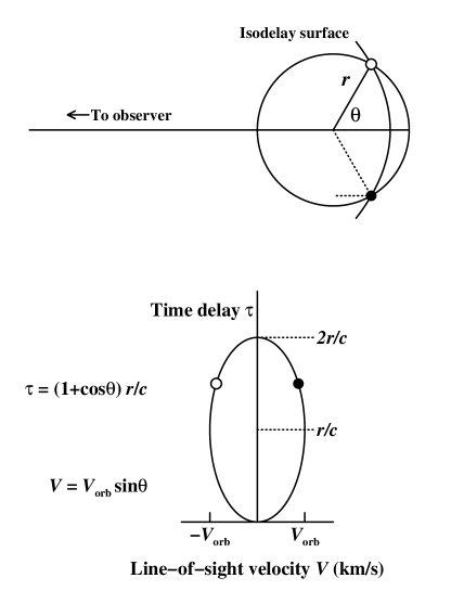
Figure 1: Upper diagram: In this simple, illustrative model, the line-emitting clouds are taken to be on a circular orbit of radius $r$ around the central black hole. The observer is to the left. In response to an instantaneous continuum outburst, the clouds seen by the distant observer at a time delay $\tau$ after detection of the continuum outburst will be those that lie along an “isodelay surface,” for which the time delay relative to the continuum signal will be $\tau=(1+\cos\theta)r/c$, the length of the dotted path shown. Lower diagram: The circular orbit is mapped into the line-of-sight velocity/time-delay plane.

We can now construct a simple velocity delay map. Consider the trivial case of BLR that is comprised of an edge-on (inclination 90^o) ring of clouds in a circular Keplerian orbit, as shown on the top panel of Figure 1. In the lower panel of Figure 1, we map the points from polar coordinates in configuration space to points in velocity-time delay space. Points ($r$, $\theta$) in configuration space map into line-of-sight velocity/time-delay space ($V$, $\tau$) according to $V=-V_{\rm orb}\sin\theta$, where $V_{\rm orb}$ is the orbital speed, and $\tau=(1+\cos\theta)r/c$. Inspection of Figure 1 shows that a circular Keplerian orbit projects to an ellipse in velocity-time delay space. Generalization to radially extended geometries is simple: a disk is a system of rings of different radii and a spherical shell is a system of rings of different inclinations. Figure 2 shows a system of circular Keplerian orbits, i.e., $V_{\rm orb}(r)\propto r^{-1/2}$, and how these project into velocity-delay space. A key feature of Keplerian systems is the “taper” in the velocity-delay map with increasing time delay.

Figure 2: This diagram is similar to Figure 1. Here we show how circular Keplerian orbits of different radii map into the velocity-time delay plane. Inner orbits have a larger velocity range ($V\propto r^{-1/2}$) and shorter range of time delay ($\tau_{\rm max}=2r/c$), resulting in tapering of the map in velocity with increasing time delay, a general feature of gravitationally dominated systems.

In Figure 3, we show two complete velocity-delay maps for radially extended systems, in one case a Keplerian disk and in the other a spherical system of clouds in circular Keplerian orbits of random inclination. In both examples, the velocity-delay map is shown in the upper left panel in greyscale. The lower left panel shows the result of integrating the velocity-delay map over time delay, thus yielding the emission-line profile for the system. The upper right panel shows the result of integrating over velocity, yielding the total time response of the line; this is referred to as the “delay map” or the “one-dimensional transfer function.” Inspection of Figure 3 shows that these two velocity-delay maps are superficially similar; both show clearly the tapering with time delay that is characteristic of Keplerian systems and have double-peaked line profiles. However, it is also clear that they can be easily distinguished from one another. This, of course, is the key: the goal of reverberation mapping is to use the observables, namely the continuum light curve $C(t)$ and the emission-line light curve $L(V,t)$ and invert eq. (2) to recover the velocity-delay map $\Psi(V,\tau)$. Equation (2) represents a fairly common type of problem that arises in many applications in physics and engineering. Indeed, the velocity-delay map is the Green’s function for the system. Solution of eq. (2) by Fourier transforms immediately suggests itself, but real reverberation data are far too sparsely sampled and usually too noisy to this method to be effective. Other methods have to be employed, such as reconstruction by the maximum entropy method (Horne 1994). Unfortunately, even the best reverberation data obtained to date have not been up to the task of yielding a high-fidelity velocity-delay map. Existing velocity-delay maps are noisy and ambiguous. Figure 4 shows the result of an attempt to recover a velocity-delay map for the C iv–He ii spectral region in NGC 4151 (Ulrich & Horne 1996). The Keplerian taper of the map is seen, but other possible structure is only hinted at, as it is in other attempt to recover a velocity-delay map from real data (e.g., Wanders et al. 1995; Done & Krolik 1996; Kollatschny 2003). It must be pointed out, however, that no case to date has recovery of the velocity-delay map been a design goal for an experiment. Previous reverberation-mapping experiments have had the more modest goal of recovering only the mean response time of emission lines, from which one can still draw considerable information. By integrating eq. (2) over velocity and then convolving it with the continuum light curve, we find that under reasonable conditions, cross-correlation of the continuum and emission-line light curves yields the mean response time, or “lag,” for the emission lines.

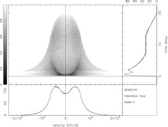
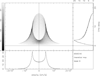
Figure 3: Theoretical velocity-delay maps $\Psi(V,\tau)$ shown in greyscale for a spherical distribution of line-emitting clouds in circular Keplerian orbits of random inclination (left) and an inclined Keplerian disk of line-emitting clouds (right). Projections in velocity and time-delay show the line profile (below) and delay map (right). From Horne et al. (2004).

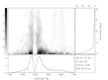
Figure 4: A velocity–delay map for the C iv–He ii region in NGC 4151, based on data obtained with the International Ultraviolet Explorer. From Ulrich & Horne (1996).

3 Reverberation Results

Prior to about 1988, there were a large number of observations that suggested that the broad emission lines in Seyferts varied in response to continuum variations and did so on surprisingly short time scales. These early results led to the first highly successful reverberation campaign, carried out in 1988–89, combining UV spectra obtained with the International Ultraviolet Explorer (IUE) with ground-based optical observations from numerous observatories. The program ran for over 8 months and achieved time resolution of a few days in several continuum and emission-line time series (Clavel et al. 1991; Peterson et al. 1991; Dietrich et al. 1993; Maoz et al. 1993). A number of important results were produced by this project, including:

1. From the shortest measured wavelength (1350 Å) to the longest (5100 Å), the continuum variations appear to be in phase, with any lags between bands amounting to no more than a couple of days.

2. The highest ionization emission lines respond most rapidly to continuum variations (e.g., $\sim 2$ days for He ii $\,\lambda 1640$ and $\sim 10$ days for Ly$\alpha$ and C iv $\lambda 1549$) and the lower ionization lines respond less rapidly (e.g., $\sim 20$ days for H$\beta$ and nearly 30 days for C iii] $\lambda 1909$). The BLR thus shows radial ionization stratification.

Optical spectroscopic monitoring of NGC 5548 continued for a total of 13 years, and during the fifth year of the program (1993), concurrent high-time resolution (daily observations) were made for about 60 days with IUE and for 39 days with the Faint Object Spectrograph on Hubble Space Telescope (Korista et al. 1995). Over time, it became clear that the H$\beta$ emission-line lag is a dynamic quantity, it varies with time and is dependent on the current mean continuum luminosity (Peterson et al. 2002). In other words, there is much more nuclear gas on scales of thousands of gravitational radii than previously thought: at any given time, most of the emission in any particular line arises primarily in that gas for which the physical conditions optimally produce that particular emission line (cf. the “locally optimized cloud” model of Baldwin et al. 1995).

Peterson et al. (2004) recently completed a comprehensive reanalysis of 117 independent reverberation mapping data sets on 37 AGNs, measuring emission-line lags, line widths, and black hole masses for all but two of these sources. Calibration of the reverberation-based mass scale, as embodied in the scaling factor $f$ in eq. (1), is set by assuming that AGNs follow the same relationship between black hole mass and the host-galaxy bulge velocity dispersion (the $M_{\rm BH}-\sigma_{*}$ relationship) seen in quiescent galaxies (Onken et al. 2004). The range of measured masses runs from $\sim 2\times 10^{6}\,M_{\odot}$ for the narrow-line Seyfert 1 galaxy NGC 4051 to $\sim 1.3\times 10^{9}\,M_{\odot}$ for the quasar PG 1426+015. The statistical errors in the mass measurements (due to uncertainties in lag and line-width measurement) are typically only about 30%. However, the systematic errors, due to scatter in the $M_{\rm BH}-\sigma_{*}$ relationship, amount to about a factor of three; this systematic uncertainty can decreased only by understanding the geometry and kinematics of the BLR. Figure 5 shows a current version of the mass-luminosity relationship for AGNs, based on these reverberation-based black hole masses.

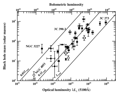
Figure 5: Black hole mass vs. luminosity for 35 reverberation-mapped AGNs. The luminosity scale on the lower x-axis is $\log\lambda L_{\lambda}$ in units of ergs s^-1. The upper x-axis shows the bolometric luminosity assuming that $L_{\rm bol}\approx 9\lambda L_{\lambda}$. The diagonal lines show the Eddington limit $L_{\rm Edd}$, $0.1L_{\rm Edd}$, and $0.01L_{\rm Edd}$. The open circles represent narrow-line Seyfert 1 galaxies. From Peterson et al. (2004).

4 The Future: What Will It Take to Map the Broad-Line Region?

While we still do not have a velocity-delay map in hand, we certainly know how to get one. More than a dozen years of experience in reverberation mapping have led to a reasonably good understanding of the timescales for response of various lines as a function of luminosity and of how the continuum itself varies with time. On the basis of this information, we have carried out extensive simulations to determine the observational requirements to obtain high-fidelity velocity-delay maps for emission lines in moderate luminosity Seyfert galaxies (quantities that follow are based specifically on NGC 5548, by far the AGN best studied by reverberation). A sample numerical simulation is shown in Figure 6. As described more completely by Horne et al. (2004), the principal requirements are:

1. High time resolution, (less than 0.2–1 day, depending on the emission line). The interval between observations translates directly into the resolution in the time-delay axis.

2. Long duration (several months). A rule of thumb in time series analysis is that the duration of the experiment should exceed the maximum timescale to be probed by at least a factor of three. The lag for H$\beta$ in NGC 5548 is typically around 20 days, so the longest timescale to be probed is $2r/c$. The duration should thus be at least $\sim 120$ days to map the H$\beta$-emitting region. However, since C iv seems to respond twice as fast as H$\beta$, the C iv-emitting region might be mapped in as little as $\sim 60$ days. A more important consideration, however, is detection in the time series a strong continuum signal, such as a change in sign of the derivative of the light curve. This produces a similarly strong emission-line response. We find that $\sim 200$ days of observations are required to be certain that such an event occurs, and to observe its consequences in the emission lines.

3. Moderate spectral resolution ($\leq 600$ km s^-1). While higher spectral resolution is always desirable, AGN emission lines show little additional structure at resolution better than several hundred kilometers per second. Higher resolution does, however, make it in principle possible to detect a gravitational redshift (e.g., Kollatschy 2004), providing an independent and complementary measure of the black hole mass.

4. High homogeneity and signal-to-noise ratios ($S/N\approx 100$). Both continuum and emission-line flux variations are small on short time scales, typically no more than a few percent on diurnal timescales. Excellent relative flux calibration and signal-to-noise ratios are necessary to make use of the high time resolution.

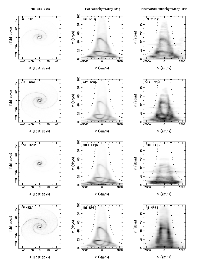
Figure 6: Numerical simulations of velocity–delay map recovery. An arbitrary but complex geometry was chosen to show that a complicated BLR structure can be recovered. The left column shows the BLR geometry in four lines, Ly$\alpha\,\lambda 1215$, C iv $\lambda 1549$, He ii $\lambda 1640$, and H$\beta\,\lambda 4861$, from top to bottom. The middle column shows the BLR model mapped into velocity–delay space. The right column shows the recovered velocity–delay map recovered from simulated data. From Horne et al. (2004).

The final point makes it clear that this will be difficult to do with ground-based observations: it is hard to maintain such high levels of homogeneity and thus accurate relative flux calibration with a variable point-spread function, such as one dominated by the effects of atmospheric seeing. Space-based observations are much more likely to succeed, and moreover, the ultraviolet part of the spectrum gives access to the important strong lines Ly$\alpha$, N v $\lambda 1240$, Si iv $\lambda 1400$, C iv $\lambda 1549$, and He ii $\lambda 1640$, all of which vary strongly.

We have carried out a series of simulations assuming specifically observation of NGC 5548 with the Space Telescope Imaging Spectrograph (STIS) on HST. We assume that the typical BLR response times are as observed during the first major monitoring campaign in 1989, as these values appear to be typical. We also assume for practical reasons that we can obtain only one observation per day (mostly on account of restrictions against the use of the STIS UV detectors during orbits when HST passes through the South Atlantic Anomaly) which we must complete in one HST orbit, using the typical time that NGC 5548 is observable per orbit. Furthermore, we included in the simulations nominal spacecraft and instrument safing events of typical duration (generally a few days) and frequency. We also considered the effects of early termination of the experiment due, for example, to a more catastrophic failure. We carried out 10 individual simulations, with each one using a different continuum model; all of the continuum models were ”conservative” in the sense that the continuum activity is weaker and less pronounced than it is usually observed to be.

Given our assumptions, we find that all 10 of the simulated experiments succeed within 200 days. For the most favorable continuum behavior, success can be achieved in as little as $\sim 60$ days, though this is rare, or more commonly in around $\sim 150$  days. We also find that these results are robust against occasional random data losses.

These generally conservative assumptions argue strongly that velocity-delay maps for all the strong UV lines in NGC 5548 could be obtained in a 200-orbit HST program based on one orbit per day. There are clearly elements of risk associated with the program, the most obvious being early termination on account of a systems failure or a major safing event that would end the time series prematurely. This risk is somewhat mitigated by the conservatism of our simulations; it is possible that the experiment could succeed in much less time. Indeed, if we define “success” as obtaining a velocity-delay map that is stable for 50 days, we find that the probability of success is as high as $\sim 90$% in 150 days.

Finally, one might also ask about the scientific risk: for example, what if the velocity-delay map, though of high fidelity, cannot be interpreted? In other words, what if the velocity-delay map is a “mess” and has no discernible structure? First of all, this is not a likely outcome since long-term monitoring shows persistent features in emission-line profiles that imply there is some order or symmetry to the BLR. Moreover, even if the BLR turns out to be a “mess” we’ll still have learned an important fact about the BLR structure, namely that it is basically chaotic. But the bottom line is that right now we have nearly complete ignorance about the BLR structure. We cannot even assess to any level of confidence how many velocity-delay maps of AGNs we will need to solve the problem until we have obtained at least one velocity-delay map of at least one emission line. Until we have that, our knowledge of the role of the BLR in AGN fueling and outflows will remain based on theoretical speculation alone, historically a very dangerous situation for astrophysicists.

5 Summary

We have argued that reverberation mapping provides a unique probe of the inner structure of AGNs. The reverberation technique has been very successful in determining the BLR sizes and black hole masses in 35 AGNs. The masses obtained are accurate to about a factor of 3, based on the observed scatter in the AGN $M_{\rm BH}-\sigma_{*}$ relationship. The accuracy of these masses is fundamentally limited by unknown geometry and kinematics of BLR. We have also argued that it is possible to obtain complete, high-fidelity velocity-delay maps of the strong ultraviolet lines in relatively nearby, moderately luminous AGNs with HST, and we specifically argue that this can be done with high confidence of success for NGC 5548 with one HST orbit per day for a period of no longer than 200 days.