The 2dF Galaxy Redshift Survey: luminosity functions by density environment and galaxy type

Abstract

We use the 2dF Galaxy Redshift Survey to measure the dependence of the b_J-band galaxy luminosity function on large-scale environment, defined by density contrast in spheres of radius $8h^{-1}$Mpc, and on spectral type, determined from principal component analysis. We find that the galaxy populations at both extremes of density differ significantly from that at the mean density. The population in voids is dominated by late types and shows, relative to the mean, a deficit of galaxies that becomes increasingly pronounced at magnitudes brighter than $M_{\rm b_{J}}-5\log_{10}h\la-18.5$. In contrast, cluster regions have a relative excess of very bright early-type galaxies with $M_{\rm b_{J}}-5\log_{10}h\la-21$. Differences in the mid to faint-end population between environments are significant: at $M_{\rm b_{J}}-5\log_{10}h=-18$ early and late-type cluster galaxies show comparable abundances, whereas in voids the late types dominate by almost an order of magnitude. We find that the luminosity functions measured in all density environments, from voids to clusters, can be approximated by Schechter functions with parameters that vary smoothly with local density, but in a fashion which differs strikingly for early and late-type galaxies. These observed variations, combined with our finding that the faint-end slope of the overall luminosity function depends at most weakly on density environment, may prove to be a significant challenge for models of galaxy formation.

1 Introduction

The galaxy luminosity function has played a central role in the development of modern observational and theoretical astrophysics, and is a well established and fundamental tool for measuring the large-scale distribution of galaxies in the universe (Efstathiou, Ellis & Peterson 1988; Loveday et al. 1992; Marzke, Huchra & Geller 1994; Lin et al. 1996; Zucca et al. 1997; Ratcliffe et al. 1998; Norberg et al. 2002a; Blanton et al. 2003a;). The galaxy luminosity function of the 2dF Galaxy Redshift Survey (2dFGRS) has been characterised in several papers: Norberg et al. (2002a) consider the survey as a whole; Folkes et al. (1999) and Madgwick et al. (2002) split the galaxy population by spectral type; De Propris et al. (2003) measure the galaxy luminosity function of clusters in the 2dFGRS; Eke et al. (2004) estimate the galaxy luminosity function for groups of different mass. Such targeted studies are invaluable if one wishes to understand how galaxy properties are influenced by external factors such as local density environment (e.g. the differences between cluster and field galaxies).

A natural extension of such work is to examine a wider range of galaxy environments and how specific galaxy properties transform as one moves between them, from the very under-dense ‘void’ regions, to mean density regions, to the most over-dense ‘cluster’ regions. In order to ‘connect the dots’ between galaxy populations of different type and with different local density a more comprehensive analysis needs to be undertaken. Although progress has been made in this regard on both the observational front (Bromley et al. 1998; Christlein 2000; Hütsi et al. 2002) and theoretical front (Peebles 2001; Mathis & White 2002; Benson et al. 2003; Mo et al. 2004), past galaxy redshift surveys have been severely limited in both their small galaxy numbers and small survey volumes. Only with the recent emergence of large galaxy redshift surveys such as the 2dFGRS and also the Sloan Digital Sky Survey (SDSS) can such a study be undertaken with any reasonable kind of precision (for the SDSS, see recent work by Hogg et al. 2003, Hoyle et al. 2003, and Kauffmann et al. 2004).

In this paper we use the 2dFGRS galaxy catalogue to provide an extensive description of the luminosity distribution of galaxies in the local universe for all density environments within the 2dFGRS survey volume. In addition, the extreme under-dense and over-dense regions of the survey are further dissected as a function of 2dFGRS galaxy spectral type, $\eta$, which can approximately be cast as early and late-type galaxy populations (Madgwick et al. 2002, see Section 2). The void galaxy population is especially interesting as it is only with these very large survey samples and volumes possible to measure it with any degree of accuracy. Questions have been raised (e.g., Peebles 2001) as to whether the standard $\Lambda$CDM cosmology correctly describes voids, most notably in relation to reionisation and the significance of the dwarf galaxy population in such under-dense regions.

This paper is organised as follows. In Section 2 we provide a brief description of the 2dFGRS and the way in which we measure the galaxy luminosity function from it. The luminosity function results are presented in Section 3, and then compared with past results in Section 4. We discuss the implications for models of galaxy formation in Section 5. Throughout we assume a $\Lambda$CDM cosmology with parameters $\Omega_{m}=0.3$, $\Omega_{\Lambda}=0.7$, and $H_{0}=100h^{-1}$kms^-1Mpc^-1.

2 METHOD

2.1 The 2dFGRS survey

We use the completed 2dFGRS as our starting point (Colless et al. 2003), giving a total of 221,414 high quality redshifts. The median depth of the full survey, to a nominal magnitude limit of $b_{\rm J}\approx 19.45$, is $z\approx 0.11$. We consider the two large contiguous survey regions, one in the south Galactic pole and one towards the north Galactic pole. To improve the accuracy of our measurement our attention is restricted to the parts of the survey with high redshift completeness ($>70\%$) and galaxies with apparent magnitude $b_{\rm J}<19.0$, well within the above survey limit (see also Appendix C). Our conclusions remain unchanged for reasonable choices of both these restrictions. Full details of the 2dFGRS and the construction and use of the mask quantifying the completeness of the survey can be found in Colless et al. (2001, 2003) and Norberg et al. (2002a).

Where possible, galaxy spectral types are determined using the principal component analysis (PCA) of Madgwick et al. (2002) and the classification quantified by a spectral parameter, $\eta$. This allows us to divide the galaxy sample into two broad classes, conventionally called late and early types for brevity. The late types are those with $\eta\geq-1.4$ that have active star formation and the early types are the more quiescent galaxy population with $\eta<-1.4$. Approximately $90\%$ of the galaxy catalogue can be classified in this way. This division at $\eta=-1.4$ corresponds to an obvious dip in the $\eta$ distribution (Section 2.4; see also Madgwick et al. 2002) and a similar feature in the $\mbox{{\rm b}${}_{\rm J}$}-\mbox{{\rm r}${}_{\rm F}$}$ colour distribution, and therefore provides a fairly natural partition between early and late types. When calculating each galaxy’s absolute magnitude we apply the spectral type dependent $k+e$ corrections of Norberg et al. (2002a); when no type can be measured we use their mean $k+e$ correction. In this way all galaxy magnitudes have been corrected to zero redshift.

2.2 Local density measurement

The 2dFGRS galaxy catalogue is magnitude limited; it has a fixed apparent magnitude limit which corresponds to a faint absolute magnitude limit that becomes brighter at higher redshifts. Over any given range of redshift there is a certain range of absolute magnitudes within which all galaxies can be seen by the survey and are thus included in the catalogue (apart from a modest incompleteness in obtaining the galaxies’ redshifts). Selecting galaxies within these redshift and absolute magnitude limits defines a volume-limited sub-sample of galaxies from the magnitude-limited catalogue (see e.g. Norberg et al. 2001, 2002b; Croton et al. 2004); this sub-sample is complete over the specified redshift and absolute magnitude ranges.

To estimate the local density for each galaxy we first need to establish a volume-limited density defining population (DDP) of galaxies. This population is used to fix the density contours in the redshift space volume containing the magnitude-limited galaxy catalogue. We restrict the magnitude-limited survey to the redshift range $0.05<z<0.13$, giving an effective sampling volume of approximately $7\times 10^{6}h^{-3}$Mpc³. Such a restriction guarantees that all galaxies in the magnitude range $-19>M_{\rm b_{J}}-5\log_{10}h>-22$ (i.e. effectively brighter than $M^{*}+0.7$) are volume limited, and allows us to use this sub-population as the DDP. The mean number density of DDP galaxies is $8.6\times 10^{-3}h^{3}$Mpc^-3. In Appendix B we consider the effect of changing the magnitude range of the DDP and find only a very small difference in our final results.

The local density contrast for each magnitude-limited galaxy is determined by counting the number of DDP neighbours within an $8h^{-1}$Mpc radius, $N_{g}$, and comparing this with the expected number, $\bar{N_{g}}$, obtained by integrating under the published luminosity 2dFGRS function of Norberg et al. (2002a) over the same magnitude range that defines the DDP:

$$\delta_{8}\equiv\frac{\delta\rho_{g}}{\rho_{g}}=\frac{N_{g}-\bar{N_{g}}}{\bar{N_{g}}}\ \Bigg{|}_{R=8h^{-1}\rm{Mpc}}~{}.$$ (1)

In Appendix B we explore the effect of changing this smoothing scale from between $4h^{-1}$Mpc to $12h^{-1}$Mpc. We find that our conclusions remain unchanged, although, not surprisingly, smaller scale spheres tend to sample the under dense regions differently. Spheres of $8h^{-1}$Mpc are found to be the best probe of both the under and over-dense regions of the survey.

With the above restrictions, the magnitude-limited galaxy sample considered in our analysis contains a total of $81,387$ ($51,596$) galaxies brighter than $M_{\rm b_{J}}-5\log_{10}h=-17~{}(-19)$, with $30,354$ ($23,043$) classified as early types and $42,772$ ($23,815$) classified as late types. Approximately $70\%$ of all galaxies in this sample are sufficiently within the survey boundaries to be given a local density. Details of the different sub-samples binned by local density and type are given in Table 1.

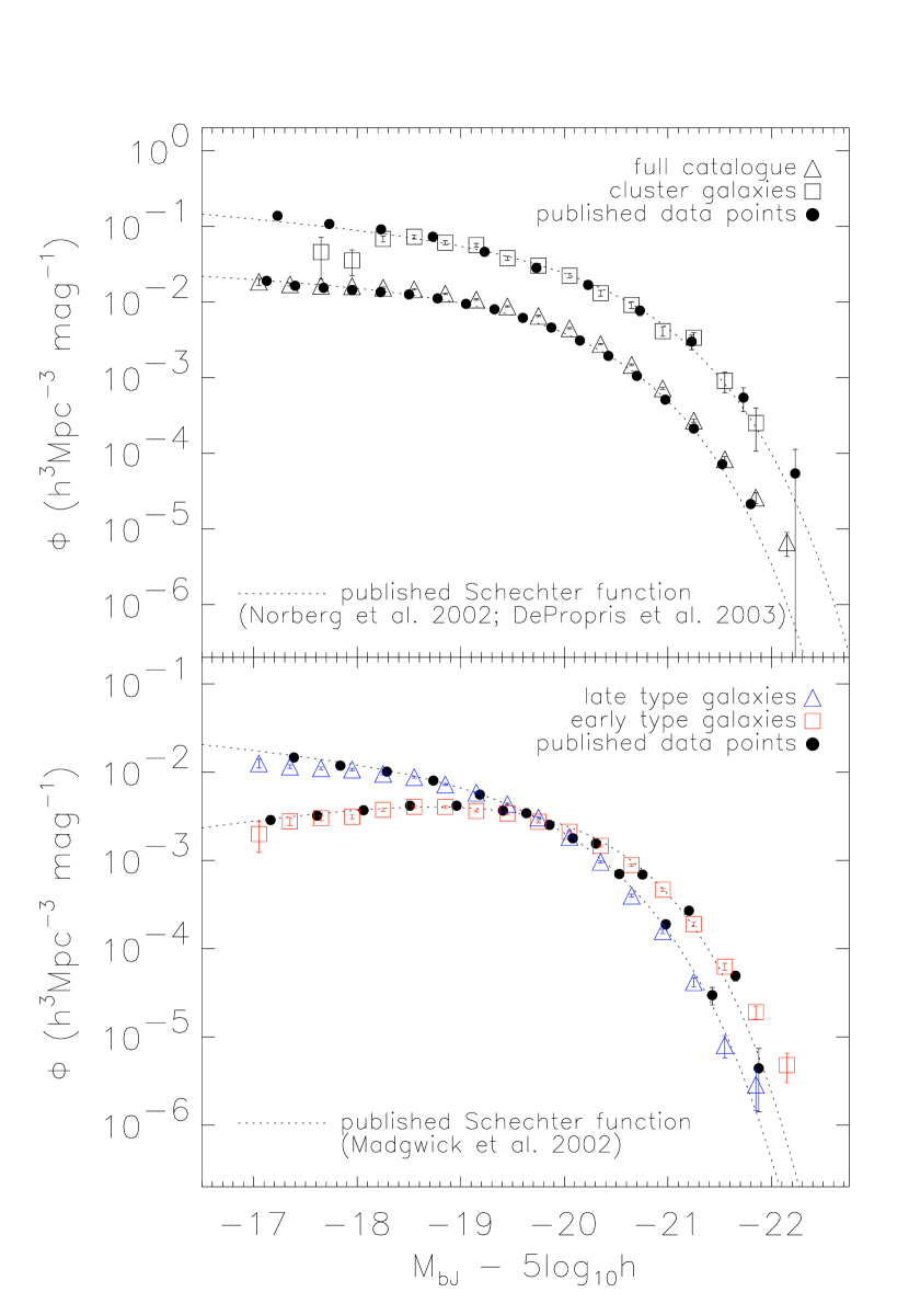
Figure 1: A comparison of the published 2dFGRS luminosity function (circles and dotted lines) to that calculated by our joint SWML(shape)/CiC(normalisation) method (squares and triangles) for select galaxy samples. Shown are the (top) full catalogue luminosity function (Norberg et al. 2002a) and cluster galaxy population luminosity function (De Propris et al. 2003), and (bottom) the luminosity function for early and late-type galaxy sub-samples separately (Madgwick et al. 2002).

2.3 Measuring the luminosity function

The luminosity function, giving the number density of galaxies as a function of luminosity, is conveniently approximated by the Schechter function (Schechter 1976, see also Norberg et al. 2002a):

$$d\phi=\phi^{*}{(L/L^{*})}^{\alpha}\exp(-L/L^{*})\ d(L/L^{*})~{},$$ (2)

dependent on three parameters: $L^{*}$ (or equivalently $M^{*}$), providing a characteristic luminosity (magnitude) for the galaxy population; $\alpha$, governing the faint-end slope of the luminosity function; and $\phi^{*}$, giving the overall normalisation. Our method, which we describe below, will be to use the magnitude-limited catalogue binned by density and type to calculate the shape of each luminosity function, draw on restricted volume-limited sub-samples of each to fix the correct luminosity function normalisation, then determine the maximum likelihood Schechter function parameters for each in order to quantify the changing behaviour between different environments.

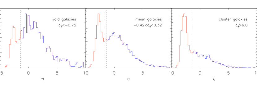
Figure 2: The distribution of the spectral parameter, $\eta$, for the void, mean, and cluster galaxies used in our analysis (Table 1). The vertical dotted line at $\eta=-1.4$ divides the quiescent galaxy population (early types on left) from the more active star-forming galaxies (late types on right). From void to cluster environment, the dominant galaxy population changes smoothly from late-type to early-type.

The luminosity function shape is determined in the standard way using the step-wise maximum likelihood method (SWML Efstathiou, Ellis & Peterson 1988) and the STY estimator (Sandage, Tammann & Yahil 1979). See Norberg et al. (2002a) for a complete description of the application of these two techniques to the 2dFGRS. All STY fits are performed over the magnitude range $-17>M_{\rm b_{J}}-5\log_{10}h>-22$.

Such techniques fail to provide the luminosity function normalisation, however, and one needs to consider carefully how to do this when studying galaxy populations in different density environments. To normalise each luminosity function we employ a new counts in cells (CiC) technique which directly calculates the number density of galaxies as a function of galaxy magnitude from the galaxy distribution. Briefly, this is achieved by counting galaxies in restricted volume-limited sub-regions of the survey. We discuss our CiC method in more detail in Appendix A. As we show there, when galaxy numbers allow a good statistical measurement the luminosity function shape determined by the SWML and CiC methods agree very well. As the SWML estimator draws from the larger magnitude-limited survey rather than the smaller CiC volume-limited sub-samples, we choose the above two-step SWML/CiC approach rather than the CiC method alone to obtain the best results for each luminosity function. Once the CiC luminosity function has been calculated for the same galaxy sample, the SWML luminosity function is then given the correct amplitude by requiring that the number density integrated between the magnitude range $-19>M_{\rm b_{J}}-5\log_{10}h>-22$ be the same as that for the CiC result.

2.4 Comparison to previous 2dFGRS results

In Fig. 1 we give a comparison of our measured luminosity functions for selected galaxy populations with the equivalent previously-published 2dFGRS results (see each reference for complete details). These include (top panel) the full survey volume (Norberg et al. 2002a) and cluster galaxy luminosity functions (De Propris et al. 2003), and (bottom panel) the luminosity functions derived for late and early-type galaxy populations separately (Madgwick et al. 2002). For all, the squares and triangle symbols show our hybrid SWML/CiC values while the circles and dotted lines give the corresponding published 2dFGRS luminosity function data points and best Schechter function estimates, respectively. The close match between each set of points confirms that our method is able to reproduce the published 2dFGRS luminosity shape and amplitude successfully.

There are a few points to note. Firstly, the cluster luminosity function is not typically quoted with a value of $\phi^{*}$ since the normalisation of the cluster galaxy luminosity distribution will vary from cluster to cluster (dependent on cluster richness). Because of this we plot the De Propris et al. cluster luminosity function using our $\phi^{*}$ value.

Secondly, the Madgwick et al. early and late-type galaxy absolute magnitudes include no correction for galaxy evolution, which, if included, would have the effect of dimming the galaxy population somewhat. We have checked the significance of omitting the evolution correction when determining the galaxy absolute magnitudes and typically find only minimal differences in our results and no change to our conclusions.

Thirdly, the STY Schechter function values we measure tend to present a slightly ‘flatter’ faint-end slope than seen for the full survey: our all-type STY estimate returns $\alpha=-1.05\pm 0.02$ (Table 1) whereas for the completed survey (across the redshift range $0.02<z<0.25$) the recovered $\alpha$ value is $-1.18\pm 0.02$ (Cole et al. in preparation). This difference is due primarily to three systematic causes: the minimum redshift cut required to define the DDP which results in a restricted absolute magnitude range over which we can measure galaxies; the non-perfect description of the galaxy luminosity function by a Schechter function together with the existing degeneracies in the $M^{*}-\alpha$ plane; the sensitivity of the faint-end slope parametrisation to model dependent corrections for missed galaxies. For our results, these systematic effects do not hinder a comparison between sub-samples, but it is essential to take into account the different cuts we imposed for any detailed comparison with other works. In Appendix C we discuss these degeneracies and correlations further. We test their influence by fixing each $\alpha$ at the published field value when applying the STY estimator and find a typical variation of less than $0.2$ magnitudes in $M^{*}$ from the main results presented in Section 3. Such systematics do not change our conclusions.

Lastly, the 2dFGRS photometric calibrations have improved since earlier luminosity function determinations, and thus the good match seen in Fig. 1 demonstrates that the new calibrations have not significantly altered the earlier results.

In Fig. 2 we show the $\eta$ distribution for our void, mean, and cluster galaxy samples. The mean galaxy distribution is essentially identical to that shown in Fig. 4 of Madgwick et al. (2002) for the full survey, demonstrating that the mean density regions contain a similar mix of galaxy types to that of the survey as a whole. For under-dense regions late types progressively dominate, while the converse is true in the over-dense regions. This behaviour can be understood in terms of the density-morphology relation (e.g. Dressler 1980), and will be explored in more detail in the next section.

Figure 3: (top) The SWML luminosity functions for the 2dFGRS galaxy catalogue in regions of the survey of varying density contrast, $\delta_{8}$, from void to mean density to cluster. The best-fit Schechter function parameters for each are given in Table 1 and the corresponding Schechter function curves are over plotted here with dotted lines. (bottom) The void and cluster luminosity functions normalised to the mean luminosity function so as to highlight the relative differences in the shape of each distribution. The solid lines and bounding dotted lines show the appropriate Table 1 Schechter functions normalised to the mean Schechter function and $1\sigma$ uncertainty.

Table 1: Properties of our magnitude-limited galaxy samples, split by spectral type (all, early and late) and in seven density ranges (defined by $\delta_{8_{\rm{min}}}$ and $\delta_{8_{\rm{max}}}$, the density contrast in spheres of radius $8h^{-1}$Mpc). The all-type sample is also split into an ‘extreme void’ sample. $\rm{N_{GAL}}$ and $f_{\rm{VOL}}$ are the number of galaxies in each density bin and the volume fraction these galaxies occupy, respectively. $f_{\rm{VOL}}$ is given for all galaxy types only: early/late-type density populations are just sub-divisions of the associated all-type sample. $M^{*}$ and $\alpha$ are the likelihood estimated Schechter function parameters, and $\phi^{*}$ the associated normalisation. The integrated luminosity density, as defined by Eq. 3 with $L_{min}=0$, is given in the last column. All errors on the derived parameters reflect only the associated statistical uncertainty.

Galaxy	Galaxy	$\delta_{8_{\rm min}}$	$\delta_{8_{\rm max}}$	NGAL	$f_{\rm VOL}$	$M^{*}$	$\alpha$	$\phi^{*}$	$\langle\rho_{L}\rangle$
Type	Sample					$M_{b_{\rm J}}-5\log_{10}h$		$10^{-3}h^{3}$Mpc-3	$10^{8}h$L⊙Mpc-3
all types:	full volume	$-1.0$	$\infty$	$81,387$	$1.0$	$-19.65\pm 0.02$	$-1.05\pm 0.02$	$21.3\pm 0.5$	$2.10\pm 0.08$
	extreme void	$-1.0$	$-0.90$	$260$	$0.09$	$-18.26\pm 0.33$	$-0.81\pm 0.50$	$3.17\pm 0.90$	$0.08\pm 0.04$
	void	$-1.0$	$-0.75$	$1,157$	$0.20$	$-18.84\pm 0.16$	$-1.06\pm 0.24$	$3.15\pm 0.56$	$0.15\pm 0.04$
		$-0.75$	$-0.43$	$3,331$	$0.19$	$-19.20\pm 0.10$	$-0.93\pm 0.11$	$5.99\pm 0.62$	$0.36\pm 0.05$
	mean	$-0.43$	$0.32$	$11,877$	$0.30$	$-19.44\pm 0.05$	$-0.94\pm 0.05$	$11.3\pm 0.7$	$0.86\pm 0.07$
		$0.32$	$2.1$	$21,989$	$0.24$	$-19.64\pm 0.04$	$-0.99\pm 0.04$	$22.9\pm 1.0$	$2.16\pm 0.13$
		$2.1$	$6.0$	$15,656$	$0.07$	$-19.85\pm 0.05$	$-1.09\pm 0.04$	$49.0\pm 3.0$	$5.95\pm 0.49$
	cluster	$6.0$	$\infty$	$3,175$	$0.01$	$-20.08\pm 0.13$	$-1.33\pm 0.11$	$60.7\pm 13.2$	$11.6\pm 3.4$
late type:	full volume	$-1.0$	$\infty$	$42,772$	$-$	$-19.30\pm 0.03$	$-1.03\pm 0.03$	$15.0\pm 0.5$	$1.06\pm 0.05$
	void	$-1.0$	$-0.75$	$855$	$-$	$-18.78\pm 0.19$	$-1.14\pm 0.24$	$2.42\pm 0.55$	$0.11\pm 0.04$
		$-0.75$	$-0.43$	$2,249$	$-$	$-19.07\pm 0.12$	$-0.95\pm 0.14$	$4.54\pm 0.58$	$0.25\pm 0.05$
	mean	$-0.43$	$0.32$	$7,261$	$-$	$-19.24\pm 0.07$	$-1.00\pm 0.07$	$8.03\pm 0.61$	$0.53\pm 0.06$
		$0.32$	$2.1$	$11,921$	$-$	$-19.36\pm 0.06$	$-1.04\pm 0.05$	$15.5\pm 1.0$	$1.17\pm 0.11$
		$2.1$	$6.0$	$7,596$	$-$	$-19.37\pm 0.07$	$-1.03\pm 0.07$	$36.3\pm 2.9$	$2.73\pm 0.31$
	cluster	$6.0$	$\infty$	$1,316$	$-$	$-19.34\pm 0.18$	$-1.09\pm 0.20$	$54.0\pm 12.2$	$4.09\pm 1.31$
early type:	full volume	$-1.0$	$\infty$	$30,354$	$-$	$-19.65\pm 0.03$	$-0.65\pm 0.03$	$8.80\pm 0.22$	$0.75\pm 0.03$
	void	$-1.0$	$-0.75$	$220$	$-$	$-18.62\pm 0.33$	$-0.15\pm 0.53$	$0.67\pm 0.10$	$0.02\pm 0.01$
		$-0.75$	$-0.43$	$861$	$-$	$-19.16\pm 0.14$	$-0.43\pm 0.24$	$1.62\pm 0.17$	$0.88\pm 0.02$
	mean	$-0.43$	$0.32$	$3,873$	$-$	$-19.38\pm 0.08$	$-0.39\pm 0.11$	$4.13\pm 0.19$	$0.27\pm 0.02$
		$0.32$	$2.1$	$8,809$	$-$	$-19.59\pm 0.05$	$-0.52\pm 0.06$	$10.6\pm 0.4$	$0.84\pm 0.05$
		$2.1$	$6.0$	$7,163$	$-$	$-19.89\pm 0.06$	$-0.81\pm 0.06$	$24.2\pm 1.6$	$2.67\pm 0.23$
	cluster	$6.0$	$\infty$	$1,731$	$-$	$-20.13\pm 0.18$	$-1.12\pm 0.14$	$37.1\pm 7.7$	$6.00\pm 1.75$

3 RESULTS

3.1 Luminosity functions

The top panel of Fig. 3 shows the 2dFGRS galaxy luminosity function estimated for the six logarithmically-spaced density bins and additional extreme void bin, $\delta_{8}<-0.9$, given in Table 1. The luminosity function varies smoothly as one moves between the extremes in environment. Each curve shows the characteristic shape of the Schechter function, for which we show the STY fit across the entire range of points plotted with dotted lines. The Schechter parameters are given in Table 1, along with the number of galaxies considered in each density environment and the volume fraction they occupy. A number of points of interest regarding the variation of these parameters with local density will be discussed below.

To examine the relative differences in the void and cluster galaxy populations with respect to the mean, in the bottom panel of Fig. 3 we plot the ratio of the void and cluster luminosity functions to the mean luminosity function. Also shown is the ratio of the corresponding Schechter functions to the mean Schechter function (solid lines) and $1\sigma$ uncertainty (dotted lines, where only the error in $M^{*}$ and $\alpha$ has been propagated). For a non-changing luminosity function shape, this ratio is a flat line whose amplitude reflects the relative abundance of the samples considered. For two Schechter functions differing in both $\alpha$ and $M^{*}$, the faint-end of the ratio is most sensitive to the differences in $\alpha$ and the bright end to the differences in $M^{*}$. We note that the error regions on the Schechter function fits shown here do not include the uncertainty of the mean sample, as the correlation of its error with the other samples is unknown. This panel reveals significant shifts in abundances at the bright end: in voids there is an increasing deficit of bright galaxies for magnitudes $M_{\rm b_{J}}-5\log h\la-18.5$, while clusters exhibit an excess of very luminous galaxies at magnitudes $M_{\rm b_{J}}-5\log h\la-21$.

It is well-established that early and late-type galaxy populations have very different luminosity distributions (Fig. 1). In Fig. 4 we explore the density dependence of these populations. The upper panels show the luminosity functions and their Schechter function fits, as in Fig. 3, but for (left panel) early types and (right panel) late types separately. In the corresponding lower panels we show the ratio of each extreme density population to the mean density luminosity function, following the same format as the bottom panel of Fig. 3. (We note that the mean luminosity functions for each type used in this figure are both very similar in shape to that shown in the bottom panel of Fig. 1). The best-fit Schechter parameters are given in Table 1. Again we see a smooth transition in the galaxy luminosity function as one moves through regions of different density contrast. The lower left panel of Fig. 4 shows a significant variation of the bright end early-type galaxy population with respect to the mean, while at the faint end the changes are more ambiguous, but with Schechter fits that suggest some evolution into the denser regions. Note that, although the faint end of our early-type cluster Schechter function is primarily constrained by the mid-luminosity galaxies in the sample, our maximum liklihood Schechter parameters are quite close to that found by De Propris et al. (2003) for a comparable galaxy population but measured approximately three magnitudes fainter. In contrast to the early types, in the lower right panel of Fig. 4 late-type galaxies show little change in relative population between the mean and cluster environments and a possible “tilt” favouring the faint-end for low-density environments. Due to deteriorating statistics we do not consider the type dependent extreme void luminosity function which was introduced in Fig. 3.

The essence of our results is best appreciated when we directly compare the early and late-type galaxy distributions, separately for the cluster and void regions of the survey, as shown in Fig. 5. This figure reveals a striking contrast: the void population is composed primarily of medium to faint luminosity late-type galaxies, while for the cluster population early types dominate down to all but the faintest magnitude considered. This is the central result of our study, and shows the crucial role of accurately determining the amplitude of the luminosity function, since the shape alone does not necessarily determine the dominant population of a region.

Figure 4: Comparing both the (top) absolute and (bottom) relative distributions of (left) early-type galaxies in different density environments, and (right) late-type galaxies in different density environments. In the bottom panels the luminosity functions have again been normalised to the mean (each to their respective type) as done previously in Fig. 3 (note that the shape of the mean for each type is very similar to that shown in Fig. 1). Here the solid lines and bounding dotted lines show the appropriate Table 1 Schechter functions normalised to the mean Schechter function and $1\sigma$ uncertainty.

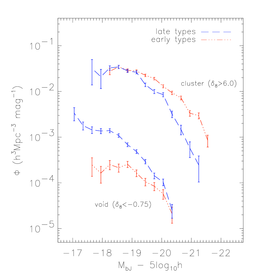
Figure 5: A direct comparison of the early and late-type galaxy populations in the cluster environment (top two luminosity functions) and void regions of the survey (bottom two luminosity functions). The void population is composed almost exclusively of faint late-type galaxies, while in the clusters regions the galaxy population brighter than $M_{\rm b_{J}}-5\log_{10}h=-19$ consists predominantly of early types.

3.2 Evolution with environment

It is well known that the Schechter function parameters are highly correlated. In Fig. 6 we show the $1\sigma$ ($68\%$ $2$-parameter) and $3\sigma$ ($99\%$ $2$-parameter) $\chi^{2}$ contours in the $M^{*}-\alpha$ plane for the early-type, late-type, and combined type cluster and void populations. For a given spectral type, all show a greater than $3\sigma$ difference in the STY Schechter parameters between the void and cluster regions. Intermediate density bins are omitted for clarity but follow a smooth progression with smaller error ellipses between the two extremes shown. In Appendix C we explore in more detail the $M^{*}-\alpha$ degeneracy and confirm that our results are robust.

Our findings show that the galaxy luminosity function changes gradually with environment. We quantify this behaviour in Fig. 7 by plotting the variation of $M^{*}$ and $\alpha$ as a function of density contrast, where points to the left of $\delta_{8}=0$ represent the under-dense to void regions in the survey, and points to the right of this are measured in the over-dense to cluster regions. Late-type galaxies display a consistent luminosity function across all density environments, from sparse voids to dense clusters, with a weak dimming of $M^{*}$ in the under-dense regions, and an almost constant faint-end slope. In contrast, the luminosity distribution of early-type galaxies differs sharply between the extremes in environment: $M^{*}$ brightens by approximately $1.5$ magnitudes going from voids to clusters, while the faint-end slope moves from $\alpha\approx-0.3$ in under-dense regions to around $\alpha\approx-1.0$ in the densest parts of the survey.

Finally, in Fig. 8 we plot the mean luminosity per galaxy, $\langle\rho_{L}\rangle/\langle\rho_{g}\rangle$, obtained by integrating the luminosity function for each set of Schechter function parameters from Table 1:

$$\langle\rho_{g}\rangle=\int^{\infty}_{L_{min}}\phi(L)\ dL~{},\ \ \ \langle\rho_{L}\rangle=\int^{\infty}_{L_{min}}\phi(L)L\ dL~{},$$ (3)

where $L_{min}$ is a somewhat arbitrary observational cutoff chosen at $M_{\rm b_{J}}-5\log_{10}h=-17$. This is both the limit down to which we confidently measure our luminosity functions, and also the limit beyond which the Schechter function no longer provides a good fit to the early-type luminosity function of Madgwick et al. (2002). The final column of Table 1 gives the total luminosity density in the various density contrast environments, computed by integrating the Schechter function with no cutoff, to allow easy comparison with past and future analyses; the contribution to the calculated $\langle\rho_{L}\rangle$ from luminosities below the observational cutoff is less than a few percent. We note that $\langle\rho_{g}\rangle$ is directly related to the density contrast, $\delta_{8}$, by definition. It is interesting to see that the early-type galaxies in Fig. 8 are, on average, about a factor of two brighter per galaxy than the late types, even though the late types dominate in terms of both number and luminosity density. For all galaxy populations, the mean luminosity per galaxy shows a remarkable constancy across the full range of density environments.

4 COMPARISON TO PREVIOUS WORK

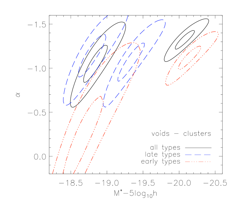
Figure 6: The $1\sigma$ ($68\%$ $2$-parameter) and $3\sigma$ ($99\%$ $2$-parameter) contours of constant $\chi^{2}$ in the $M^{*}-\alpha$ plane for the void and cluster STY estimates (in each case the void fit is on the left, corresponding to a fainter M*). Galaxy types are identified by the linestyle given in the legend. Even at the $3\sigma$ level significant differences in the void and cluster Schechter function parameters for each galaxy type can be seen.

Historically, work on the dependence of the luminosity function on large scale environment has been restricted primarily to comparisons between cluster and field galaxies, due to insufficient statistics to study voids. (Note that ‘field’ samples are usually flux-limited catalogues which cover all types of environments.) One of the aims of this work is to elucidate the properties of galaxies in void environments and understand the relationship between clusters and voids. In this section, we briefly summarise previous observations and compare them with the results presented in Section 3.

We have already shown in Fig. 1 and Section 2 that our cluster and field results are equivalent to the published 2dFGRS luminosity function results of Norberg et al. (2002a), Madgwick et al. (2002), and De Propris et al. (2003). The latter paper explains their cluster luminosity function by demonstrating that the field luminosity function can be approximately transformed into the cluster luminosity function using a simple model where the cluster environment suppresses star formation to produce a dominant bright, early-type population (see Section 4.4 of their paper for details). We expand upon such models in the next section.

Bromley et al. (1998) considered $18,278$ galaxies in the Las Campanas Redshift Survey (LCRS) as a function of spectral type and high and low local density. We confirm (e.g., Fig. 7) their qualitative finding that for early-type galaxies the faint-end slope steepens with density whereas late-type objects show little or no significant trend. We cannot make a quantitative comparison to their result because they do not give the definition of their low density sample.

Hütsi et al. (2003) use the Early Data Release of the Sloan Digital Sky Survey (SDSS) and the LCRS to consider the galaxy luminosity function as a function of density field, but in two-dimensional projection so their results are not directly comparable to ours. They find a faint-end slope of $\alpha\approx-1.1$ in all environments and an increase in $M^{*}$ of roughly $0.3$ magnitudes between the under and over-dense portions of their data. This is broadly consistent with the more detailed results obtained here with the full 2dFGRS catalogue when one averages over our two most underdense bins and three most over-dense. In separate work, these authors also consider the environmental dependence of cluster and supercluster properties in the SDSS and LCRS (Einasto et al. 2003a, 2003b). They show an almost order of magnitude increase in the mean cluster luminosity between extremes in density (defined in two dimensions by smoothing over a projected $10h^{-1}$Mpc radius around each cluster). A comparison of their results to ours (i.e. Fig. 7) suggests a correlation between galaxy, galaxy group, and galaxy cluster properties in a given density environment. A more detailed exploration would shed light on the connection between virialised objects of different mass with local density. We defer such an investigation to later work.

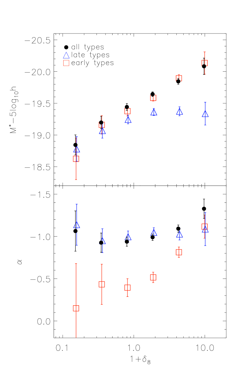
Figure 7: The maximum liklihood Schechter function $M^{*}$ and $\alpha$ parameters for each of the six density contrast regions in Table 1 (Figs. 3 and 4). Each panel shows the result for individual samples split by spectral type (early/late) and both types combined.

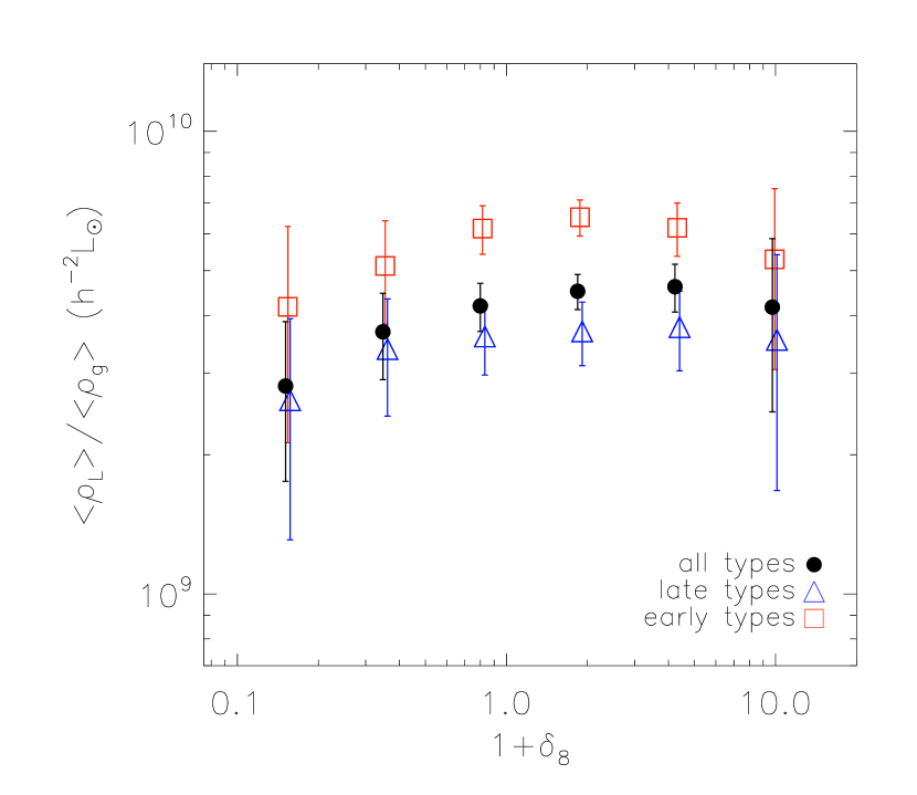
Figure 8: The mean luminosity per galaxy as a function of density environment for each galaxy type, calculated from Eq. 3 using the Schechter function parameters given in Table 1. The integral is performed by choosing $L_{min}$ so that $M_{min}-5\log_{10}h=-17$ (Section 3.2). The mean luminosity per galaxy of early types is consistently about a factor of two brighter than their late type counterparts across all density environments.

In a series of papers, members of the SDSS team undertook an analysis of the properties of galaxy samples drawn from under-dense regions in the SDSS (Rojas et al. 2004, 2003; Goldberg et al. 2004; Hoyle et al. 2003). Of most relevance to our study is the work of Hoyle et al. who completed a preliminary analysis of the SDSS void luminosity function, defined in regions of $\delta_{7}<-0.6$ using a smoothing scale of $7h^{-1}$Mpc. Their sample of $1,010$ void galaxies are typically fainter and bluer than galaxies in higher density environments but with a similar faint-end slope. Their results are consistent with what we find using a sample which contains about twice the number of void galaxies as defined by Hoyle et al.. Using the same void galaxy catalogue, Rojas et al. (2003) show that this behaviour is not merely an extrapolation of the density-morphology relationship (e.g. Dressler 1980) into sparser environments. By measuring the concentration and Sersic indices (Sersic 1968, Blanton et al. 2003b) of void and field galaxies they detect no significant shift in the morphological mix, even though their void galaxy sample is shown to be significantly bluer.

Also using the SDSS dataset, Hogg et al. (2003) consider the mean environment as a function of luminosity and colour of $115,000$ galaxies, on smoothing scales of $1$ and $8h^{-1}$Mpc. They find that their reddest galaxies show strong correlations of luminosity with local density at both the faint and bright extremes, whereas the luminosities of blue galaxies have little dependence on environment. These conclusions are consistent with the present results for our early (red) and late (blue) type luminosity functions (Fig. 7). However by restricting attention to the average environment of a galaxy of given luminosity and colour, their sample is by definition dominated by galaxies in over-dense environments. The measures they consider are therefore insensitive to one of the main questions of interest to us here, namely whether the characteristic galaxy population in the voids is distinctively different from that in other density environments. Indeed, we clearly find evidence for a population which is particularly favoured in void regions, namely faint late-type galaxies (Fig. 5).

5 DISCUSSION

Table 2: A mnemonic summary of our main results, drawing on the work of De Propris et al. (2003) and Mo et al. (2004) to interpret the observed behaviour in Figs. 5 and 7 in terms of physical processes which govern the void and cluster galaxy populations.

Region	Observation	Process
Voids		1. galaxies typically reside at the centre
	faint, late type	of low mass dark halos ($\Rightarrow$ faint)
	galaxies dominate	2. gas is available for star formation ($\Rightarrow$ blue)
		3. merger rate is low ($\Rightarrow$ spirals)
Clusters		1. typically satellite and central galaxies of
	mid-bright, early-type	massive dark halos ($\Rightarrow$ mid-bright)
	galaxies dominate	2. gas is unavailable for star formation ($\Rightarrow$ red)
		3. merger rate is high ($\Rightarrow$ ellipticals)

As clusters are comparatively well-studied objects, and have already been addressed using the 2dFGRS by De Propris et al. (2003), we focus here primarily on a discussion of the voids.

A detailed analysis of void population properties has recently become possible due to significant improvements in the quality of both theoretical modelling and observational data, as summarised by Benson et al. (2003). Peebles (2001) has argued that, visually, observed voids do not match simulated ones and discussed several statistical measures for quantifying a comparison, primarily the distance to the nearest neighbour in a reference sample. However the cumulative distributions of nearest neighbour distances shown in Figs. 4–6 of Peebles (2001) show very little difference between the reference–reference and test–reference distributions. It is not surprising that these statistical measures are insensitive to a void effect, since they are dominated by cluster galaxies. Our method is designed to overcome this difficulty by explicitly isolating the void population of galaxies so that their properties can be studied.

Motivated by the claims of discrepancies in Peebles (2001), Mathis & White (2002) investigated the nature of void galaxies using N-body simulations with semi-analytic recipes for galaxy formation. They call into question the assertion of Peebles (2001) that $\Lambda$CDM predicts a population of small haloes in the voids, concluding that “the population of faint galaxies…does not constitute a void population”. More specifically, they find that all types of galaxies tend to avoid the void regions of their simulation, down to their resolution limit of $M_{\rm B}=-16.27$ in luminosity and $M_{\rm B}=-18.46$ in morphology.

The abundance of faint galaxies we find in the void regions of the 2dFGRS seems to be at odds with the Mathis & White predictions. However their results rely on the Peebles (2001) cumulative distribution of galaxies as a function of over density (their Fig. 3) which, like cumulative distributions in general, are rather insensitive to numerically-minor components of the galaxy population. Note that Mathis & White define density contrast using the dark matter mass distribution smoothed over a $5~{}h^{-1}$Mpc sphere, whereas we measure the density contrast by galaxy counts. Another possible source of discrepancy is the uncertainties in their semi-analytic recipes, such as the implementation of supernova feedback, which can strongly effect the faint-end luminosity distribution.

There has been recent discussion in the literature about the nature of the faint-end galaxy population and its dependence on group and cluster richness. Most notably, Tully et al. (2002) show a significant steepening in the faint-end population as one considers nearby galaxy groups of increasing richness, from the Local Group to Coma. On the surface of it, this might seem at variance with our results, which are rather better described by a faint-end slope which is approximately constant with changing density environment for the full 2dFGRS galaxy sample (Fig. 7). However the steepening of the faint-end slope they find primarily occurs at magnitudes fainter than $M_{\rm B}=-17$, which is beyond the limit we can study with our sample. Also, their analysis focuses on individual groups of galaxies, while we have chosen to work with a much bigger galaxy sample and have smoothed it over a scale much larger than the typical cluster. Indeed, as discussed in Appendix B, when the smoothing scale is significantly larger than the characteristic size of the structures being probed it is possible that the Schechter function parameters may become insensitive to the small scale shifts in population. This effect, of course, would be less significant for survey regions which host clusters of clusters (i.e. super-clusters), and which are prominently seen in the 2dFGRS (Baugh et al. 2004, Croton et al. 2004). When sampling the 2dFGRS volume the trend with density that one sees using $4h^{-1}$ Mpc spheres in Fig. B1 is consistent with the Tully et al. result, although one needs to additionally understand the influences of Poisson noise.

Tully et al. attribute their results to a process of photoionisation of the IGM which suppresses dwarf galaxy formation. Over-dense regions, which at later times become massive clusters, typically collapse early and thus have time to form a dwarf galaxy population before the epoch of reionisation. Under-dense regions, on the other hand, begin their collapse at much later times and are thus subject to the photoionisation suppression of cooling baryons. This, they argue, explains the significant increase between the dwarf populations of the Local Group (low density environment) and Coma (over-dense environment). Although suggestive, a deeper understanding of what is happening will require a much more statistically significant sample.

Recently Mo et al. (2004) have considered the dependence of the galaxy luminosity function on large scale environment in their halo occupation model. In this model, the mass of a dark matter halo alone determines the properties of the galaxies. They create mock catalogues built with a halo-conditional luminosity function (Yang et al. 2003) which is constrained to reproduce the overall 2dFGRS luminosity function and correlation length for both luminosity and type. They analyse their data by smoothing over spheres of radius $8~{}h^{-1}$Mpc in their mock catalogue, and measure the luminosity function as a function of density contrast. Their work is performed in real space while we are restricted to work in redshift space. Nonetheless, their predictions qualitatively match our density-dependent luminosity functions; a quantitative comparison is deferred to subsequent work.

In the framework of the Mo et al. model, the reason the faint-end slope $\alpha$ has such a strong dependence on local density for early types (Fig. 7) is that faint ellipticals tend to reside predominantly in cluster-sized halos. The $\alpha$ dependence is weaker for late types because faint later-type galaxies tend to live primarily in less massive haloes, which are present in all density environments. The correlations between dark halo mass and the properties of the associated galaxies are not a fundamental prediction of their model, but are input through phenomenological functions adjusted to give agreement with the 2dFGRS overall luminosity functions by galaxy type. However it would be a non-trivial result if the correlations are the same independently of whether the dark matter halo is in a void or in a cluster. For instance, this property would not apply in models for which reionisation more efficiently prevented star formation in under-dense environments than in over-dense environments, as discussed above.

An interesting consequence of the Mo et al. (2004) model is that the luminous galaxy distribution (which is easy to observe but hard to model) correlates well with the dark halo mass distribution (which is hard to observe but easy to model). If their predictions prove to give a good description of the present data it will lend credence to the underlying assumption of their model—that the environmental dependence of many fundamental galaxy properties are entirely due to the dependence of the dark halo mass function on environment. Exactly why this is would still need to be explained, however such a demonstration may facilitate more detailed comparisons between theory and observation than previously possible.

An important result of our work is presented in Fig. 5, where a significant shift in the dominant population between voids and clusters is seen. Such a result points to substantial differences in the evolutionary tracks of cluster and void early-type galaxies. Cluster galaxies have been historically well studied: they are more numerous and much brighter on average, with an evolution dominated by galaxy-galaxy interactions and mergers. In voids, however, the picture is not so clear. A reasonable expectation would be that the dynamical evolution of void galaxies should be much slower due to their relative isolation, with passively evolved stellar populations and morphologies similar to that obtained during their formation. Targeted observational studies of void early-type galaxies may reveal much about the high redshift formation processes that go into making such rare objects.

Table 2 summarises our main results and provides a qualitative or mnemonic interpretation based on our observations and the work of Mo et al. (2004) and De Propris et al. (2003) (and references therein). Our primary result is the striking change in population types between voids and clusters shown in Fig. 5: faint, late-type galaxies are overwhelmingly the dominant galaxy population in voids, completely the contrary of the situation in clusters. The existence of such a population in the voids, and more generally the way populations of different type are seen to change between different density environments, place important constraints on current and future models of galaxy formation.

APPENDIX A: THE COUNTS IN CELLS LUMINOSITY FUNCTION ESTIMATOR AND COMPARISON TO THE SWML RESULTS

Our counts-in-cells (CiC) method to measure the density dependent luminosity function and obtain its amplitude is simple and will be illustrated with the example of a mock galaxy sample in a cubical volume of side-length $L$. The full luminosity function for such a sample is trivial. By definition it is simply the number of galaxies in each magnitude interval divided by the volume of the box:

$$\Phi(M)=N(M)\ /\ L^{3}~{}.$$ (A1)

To determine the luminosity function as a function of local galaxy density we require two additional pieces of information. Firstly we sub-divide the galaxy population into density bins. The local density for each galaxy is calculated within an $8h^{-1}$Mpc radius as described in Section 2.2. This gives us the number of galaxies in each density bin belonging to each magnitude range, $N_{\delta_{8}}(M)$.

Secondly we determine the volume which should be attributed to the various density bins. We do this by finding the fraction of the volume in which the galaxies of each density bin reside, $f_{\delta_{8}}$. This fraction is measured by massively oversampling the box with randomly placed $8h^{-1}$Mpc spheres, in each of which we estimate a local density in the same way as before. Once all spheres have been placed we count the number which have a local density in each density range. The volume fraction of each bin is then just the fraction of spheres found in each bin. Since the total volume of the box is known, the volume of each density bin is now also known. The density dependent luminosity function is then calculated as:

$$\phi_{\delta_{8}}(M)=N_{\delta_{8}}(M)\ /\ f_{\delta_{8}}L^{3}~{}.$$ (A2)

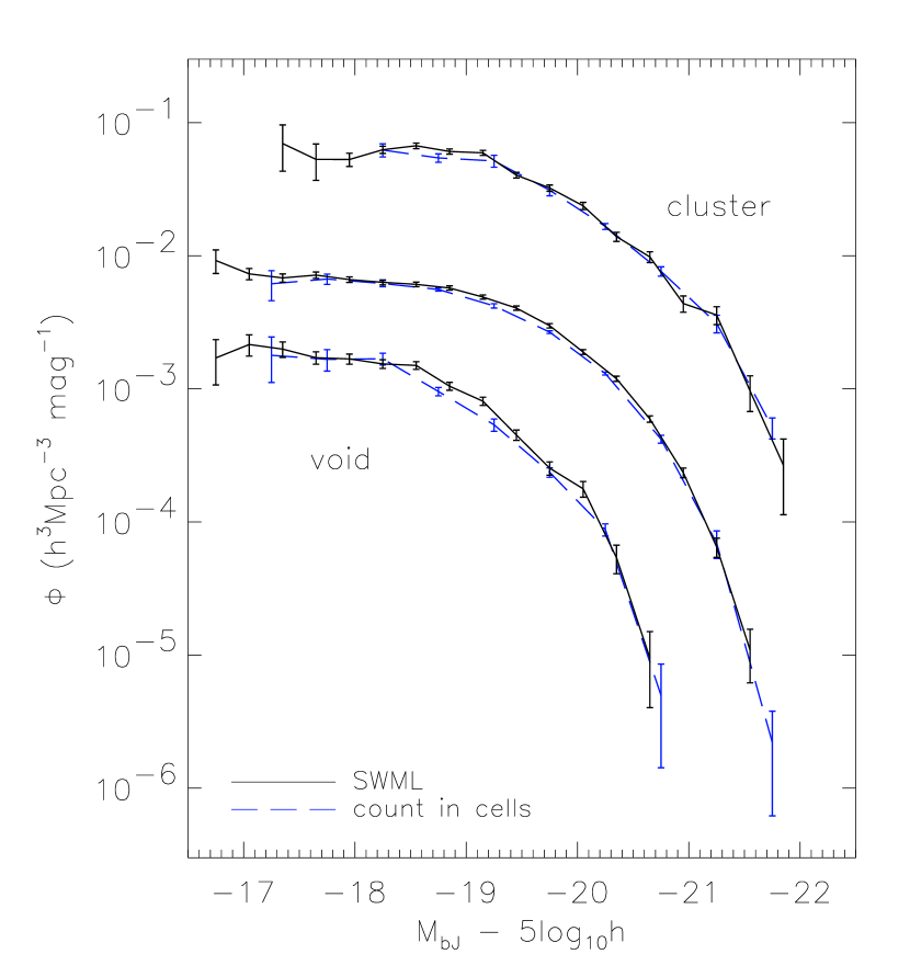
Figure A1: A comparison of the raw counts in cells luminosity function with the normalised SWML luminosity function, as described in the text (Section 2.3 and Appendix A). Shown are the cluster, mean, and void populations consisting of all galaxy types only, although all luminosity functions used in this paper behave equally as well. The shapes estimated by the two very different methods are in very good agreement over the magnitude ranges considered.

The situation becomes more complicated when dealing with a magnitude limited redshift survey instead of a simple simulated box. Galaxy counting and volume estimation must now be restricted to regions of the survey in which the magnitude range being considered is volume limited. This range of course changes for each magnitude bin in which the luminosity function is measured. In addition, small corrections ($<10\%$) are required when counting galaxies to account for the spectroscopic incompleteness of the survey (see Croton et al. 2004). In all other respects, however, the calculation of $\Phi_{\delta_{8}}(M)$ is the same as in the “box” example given above.

In Fig. A1 we show a comparison of the 2dFGRS CiC and SWML luminosity functions calculated from the same void, mean, and cluster galaxy samples. The SWML luminosity function has been normalised to the CiC measurement as described in Section 2.2. We see that both methods produce almost identical luminosity distribution shapes. This gives us confidence that the CiC luminosity function can be used to normalise the SWML luminosity function in an unbiased way.

Because of the volume-limited restriction of the CiC method, the number of galaxies used to calculate the luminosity function is smaller than for the SWML method, which draws from the larger magnitude-limited catalogue. However the benefit of the CiC method is that it gives a direct measurement of the number density of galaxies rather than just the shape of the distribution as the SWML estimator does. In addition, the CiC method is very easy to apply to mock catalogues, as described above. By combining the CiC and SWML methods we capture the best features of both.

APPENDIX B: THE EFFECTS OF CHANGING THE DENSITY DEFINING POPULATION AND SMOOTHING SCALE

In our analysis we are required to make two important choices before beginning. The first is to find the widest possible absolute magnitude range for the density defining population (DDP, see Section 2.2) while maximising the amount of the 2dFGRS survey volume sampled. The second is the scale over which we smooth the DDP galaxy distribution to determine the density contours within this volume. We will now consider the effect of changing each of these choices in turn.

The density defining population

Figure B1: The difference in the STY Schechter function parameters when the local density is calculated with an increasingly fainter density defining population (DDP): $M_{min}-5\log_{10}h=-20$, $-19$, and $-18$. Such a change also changes the redshift range of the included volume as described in the text. For clarity only results for all galaxy types are shown. The reference sample is the $M_{min}-5\log_{10}h=-19$ DDP used throughout this paper, and the other DDP results are shown relative to this.

Figure B2: The difference in the STY Schechter function parameters for different density bins when calculated by smoothing the local galaxy distribution on different scales: $4,8,$ and $12h^{-1}$Mpc. For clarity only results for all galaxy types are shown. The reference sample is the $8h^{-1}$Mpc sphere smoothing scale used throughout this paper, and the other smoothing scale results are shown relative to this.

The DDP is important in that it not only sets the mean density of galaxies used to define the density contours, but also determines the redshift range of the full magnitude-limited catalogue to be included in the analysis. Clearly one would like as high-statistics a sample as possible in as large a volume as possible for the best results. In a volume limited galaxy sample such as the DDP, the maximum galaxy redshift available is constrained by the specified faint absolute magnitude limit: galaxies beyond this redshift range are no longer guaranteed to be volume limited and are thus not included. For the DDP faint magnitude limit of $M_{min}-5\log_{10}h=-19$ the maximum survey boundary is $z=0.13$. Changing the faint magnitude limit to $M_{min}-5\log_{10}h=-18~{}(20)$, i.e. a denser (sparser) DDP, results in a maximum redshift boundary of $z=0.088~{}(0.188)$, i.e. a smaller (larger) sampling volume.

In Fig. B1 we show the result found when repeating the analysis of Section 3 (Fig. 7) but using DDPs defined by different faint absolute magnitude limits. We plot the STY $M^{*}$ and $\alpha$ values for each density bin relative to the $M_{min}-5\log_{10}h=-19$ DDP used throughout this paper. The faintest DDP shown, $M_{min}-5\log_{10}h=-18$, is approximately $8$ times denser than the brightest, $M_{min}-5\log_{10}h=-20$, but with a volume roughly $30$ times smaller. Even so, almost all measurements shown across all density bins are consistent at the $1\sigma$ level, demonstrating that our definition of the DDP is a robust representation of the underlying global density distribution.

The smoothing scale

Now let us examine how changing the smoothing scale with which we define local density affects the shape of our luminosity functions. In Fig. B2 we examine the values of the Schechter parameters when measured with spheres of radius $4$ and $12h^{-1}$Mpc, compared to when the luminosity function is measured with an $8h^{-1}$Mpc sphere.

Fig. B2 shows a typical deviation of $<0.2$ magnitudes for $M^{*}$ and $<0.2$ for $\alpha$. The $4h^{-1}$Mpc smoothing scale deviates strongly from the other values in the under-dense regions (the first two points lie beyond the axis range plotted), however in these environments such a smoothing scale gives a poor estimate of the local galaxy density due to Poisson noise in small number counts. Indeed, Hoyle et al. (2004) have shown that in the extreme under-dense 2dFGRS survey regions the characteristic scale of voids is approximately $15h^{-1}$Mpc. For cluster regions $4h^{-1}$Mpc spheres can be employed and would give a higher resolution discrimination of the structure. The $8h^{-1}$Mpc smoothing scale we have adopted captures the essential aspects of voids while roughly optimising the statistical signal, and is thus a good probe of both the under and over-dense regions of the survey volume.

APPENDIX C: SYSTEMATIC EFFECTS WHEN ESTIMATING THE SCHECHTER FUNCTION PARAMETERS

One may ask to what degree the trends seen in Fig. 7 and Table 1 are influenced by the systematics discussed in Section 2.4. We note there that our STY measurements recover a flatter faint end than the current published 2dFGRS luminosity function for the completed catalogue. We identify three systematic effects which contribute to this behaviour: the absolute magnitude range considered when applying the STY estimator, the fact that the luminosity function is not perfectly described by a Schechter function, and the sensitivity of the faint-end slope parameterisation to model-dependent corrections included to account for missed galaxies.

We find that the first two of these effects have the strongest influence on the measured STY faint-end slope. Indeed, testing the first reveals that any STY estimate of the 2dFGRS luminosity function over a restricted absolute magnitude range displays a systematic shift in the recovered STY parameters along a line in the $M^{*}-\alpha$ plane. The brighter the faint magnitude restriction, the flatter the faint-end slope is and the fainter the characteristic magnitude becomes. Such behaviour is a consequence of small but important deviations in the galaxy luminosity function shape from the pure Schechter function assumed by the STY estimator. In addition, Fig. 11 of Norberg et al. (2002) reveals a dip in the luminosity function between the magnitude range $-17>M_{\rm{b_{J}}}-5\log_{10}h>-18$ and a steepening faintward of this. In our analysis only galaxies brighter than $M_{\rm{b_{J}}}-5\log_{10}h=-17$ are considered due to the restriction of the DDP. This limitation adds extra weight to the influence of the dip on the STY fit contributing further to a flatter estimation of $\alpha$. When mock galaxy catalogues constructed to have a perfect Schechter function luminosity distribution are analysed in an identical way to the 2dFGRS samples, we find that the above systematics all but disappear and the “true” $M^{*}$ and $\alpha$ values are recovered for any reasonable choice of STY fitting range.

Finally, we note that the sensitivity of the faint-end slope parametrisation to systematic corrections for spectroscopically missed galaxies is minimised by restricting our analysis to galaxies with $\rm{b_{J}}<19$, for which the spectroscopic incompleteness is typically less than $\sim 8$% (see Fig. 16 of Colless et al. 2001).

Given that a full correction of the above systematic effects is not possible in our analysis, the next best thing we can do is try to quantify to what degree they influence our results and conclusions. We do this by fixing the faint-end slope $\alpha$ when applying the STY estimator: at $-1.2$ for the all-types samples, $-1.1$ for the late-type samples, and at $-0.5$ for the early-type samples. Such choices enforce the published field luminosity function faint end values found by Norberg et al. (2002a) and Madgwick et al. (2002) and remove the degeneracy in the $M^{*}-\alpha$ plane.

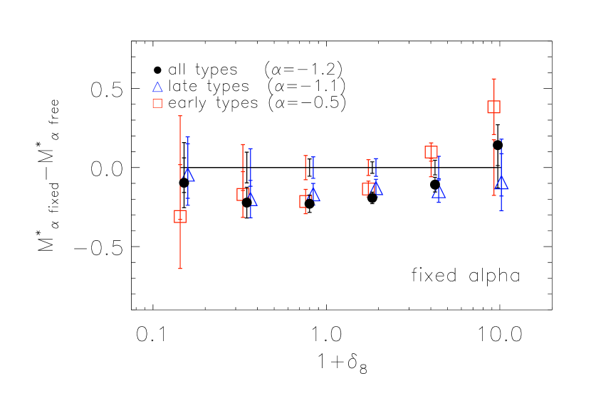
Figure C1: The shift in the STY Schechter function parameter $M^{*}$ when $\alpha$ is kept fixed at the published field value, compared with that found when $\alpha$ remains free (Table 1 and Fig. 7). The points are plotted as a function of local density and shown for each galaxy type and the combined all-type sample.

Fig. C1 shows the size of the shift in $M^{*}$ when such constraints are applied relative to that found when $\alpha$ is allowed to remain free (i.e. Table 1 and Fig. 7). Most notable here is that, apart from the two most over-dense bins in the early-type sample, there is no significant difference in the behaviour of $M^{*}$ with density environment. The approximate $0.2$ magnitude offset seen in this figure can be understood by remembering that because the faint-end slope we measure when $\alpha$ remains free is slightly flatter than the published values (due to the systematics discussed above), by artifically fixing $\alpha$ one forces $M^{*}$ to move to compensate. The important point is that the trends seen in Fig. 7 with changing local density remain unchanged.

For the two most over-dense early-type samples a shift of up to $0.4$ magnitudes is seen. We note from Table 1 that our best-fit (free $\alpha$) early-type cluster value of $\alpha=-1.12\pm 0.14$ is well matched by the equivalent 2dFGRS De Propris et al. (2003) result of $-1.05\pm 0.04$. In effect, by constraining the early-type cluster faint-end slope to the field value of $-0.5$ we ignore the real changes in galaxy population seen between the Madgwick et al. (their Fig. 10) and De Propris et al. (their Fig. 3) luminosity functions (see also our Fig. 2). Such population changes, we argue, result in the strikingly different Schechter function parameterisation behaviour seen in Fig. 7 and Table 1 for early and late-type galaxies. Fig. C1 gives us confidence that the $M^{*}-\alpha$ degeneracies and systematics investigated here are not significantly influencing our results or the conclusions we draw from them.

References

- [Baugh et al.(2004)] Baugh C. M., et al. (2dFGRS team), 2004, MNRAS, 351, L44
- [Benson, Hoyle, Torres, Vogeley(2003)] Benson A. J., Hoyle F., Torres F., Vogeley M. S., 2003, MNRAS, 340, 160
- [Blanton et al.(2003a)] Blanton M. R., et al. (SDSS team), 2003a, ApJ, 592, 819
- [Blanton et al.(2003b)] Blanton M. R., et al. (SDSS team), 2003b, ApJ, 594, 186
- [Bromley, Press, Lin, Kirshner(1998)] Bromley B. C., Press W. H., Lin H., Kirshner R. P., 1998, ApJ, 505, 25
- [Christlein(2000)] Christlein D., 2000, ApJ, 545, 145
- [Colless et al.(2001)] Colless M. et al. (2dFGRS team), 2001, MNRAS, 328, 1039
- [Colless et al.(2003)] Colless M. et al. (2dFGRS team), 2003, astro-ph/0306581
- [Croton et al.(2004)] Croton D. J., et al. (2dFGRS team), 2004, MNRAS, 352, 1232
- [De Propris et al.(2003)] De Propris R. et al. (2dFGRS team), 2003, MNRAS, 342, 725
- [Dressler (1980)] Dressler A., 1980, ApJ, 236, 351
- [Efstathiou, Ellis, Peterson(1988)] Efstathiou G., Ellis R. S., Peterson B. A., 1988, MNRAS, 232, 431
- [Einasto et al.(2003a)] Einasto J., Hütsi G., Einasto M., Saar E., Tucker D. L., Müller V., Heinämäki P., & Allam S. S. 2003a, AAP, 405, 425
- [Einasto et al.(2003b)] Einasto J., et al. 2003b, AAP, 410, 425
- [Eke et al.(2004)] Eke V. R. et al. (2dFGRS team), 2004, MNRAS, submitted (astro-ph/0402566)
- [Folkes et al.(1999)] Folkes S. et al. (2dFGRS team), 1999, MNRAS, 308, 459
- [Goldberg et al.(2004)] Goldberg D. M., Jones T. D, Hoyle F., Rojas R. R., Vogeley M. S., Blanton M. R., 2004, ApJ, submitted (astro-ph/0406527)
- [Hogg et al.(2003)] Hogg D. W. et al. (SDSS team), 2003, ApJL, 585, L5
- [Hoyle et al.(2003)] Hoyle F., Rojas R. R., Vogeley M. S., Brinkmann J., 2003, ApJ, submitted (astro-ph/0309728)
- [Hoyle & Vogeley(2004)] Hoyle, F. & Vogeley, M. S. 2004, ApJ, 607, 751
- [Hutsi et al.(2003)] Hütsi G., Einasto J., Tucker D. L., Saar E., Einasto M., Müller V., Heinämäki P., Allam S. S., 2003, A&A, submitted (astro-ph/0212327)
- [Kauffmann et al.(2004)] Kauffmann G. et al. (SDSS team), 2004, MNRAS, submitted (astro-ph/0402030)
- [Lin, Yee, Carlberg, Ellingson(1996)] Lin H., Yee H. K. C., Carlberg R. G., Ellingson E., 1996, BAAS, 28, 1412
- [Loveday, Peterson, Efstathiou, Maddox(1992)] Loveday J., Peterson B. A., Efstathiou G., Maddox S. J., 1992, ApJ, 390, 338
- [Madgwick et al.(2002)] Madgwick D. S. et al. (2dFGRS team), 2002, MNRAS, 333, 133
- [Marzke, Huchra, Geller(1994)] Marzke R. O., Huchra J. P., Geller M. J., 1994, ApJ, 428, 43
- [Mathis & White(2002)] Mathis H., White S. D. M., 2002, MNRAS, 337, 1193
- [Mo et al.(2004)] Mo H. J., Yang X., van den Bosch F. C., Jing Y. P., 2004, MNRAS, 349, 205
- [Norberg et al.(2001)] Norberg P. et al. (2dFGRS team), 2001, MNRAS, 328, 64
- [Norberg et al.(2002a)] Norberg P. et al. (2dFGRS team), 2002a, MNRAS, 336, 907
- [Norberg et al.(2002b)] Norberg P. et al. (2dFGRS team), 2002b, MNRAS, 332, 827
- [Peebles(2001)] Peebles P. J. E., 2001, ApJ, 557, 495
- [Ratcliffe, Shanks, Parker, Fong(1998)] Ratcliffe A., Shanks T., Parker Q. A., Fong R., 1998, MNRAS, 293, 197
- [Rojas et al.(2004)] Rojas R. R., Vogeley M. S., Hoyle F., Brinkmann J., 2004, ApJ, submitted (astro-ph/0409074)
- [Rojas et al.(2003)] Rojas R. R., Vogeley M. S., Hoyle F., Brinkmann J., 2003, ApJ, submitted (astro-ph/0307274)
- [Sandage et al. (1979)] Sandage A., Tammann G. A., Yahil A., 1979, ApJ, 232, 352
- [Schechter(1976)] Schechter P., 1976, ApJ, 203, 297
- [Sersic(1968)] Sersic J. L., 1968, Atlas de Galaxias Australes. Observatorio Astronómico, Córdoba.
- [Tully(2002)] Tully R. B., Somerville R. S., Trentham, N., Verheijen M. A. W., 2002, ApJ, 569, 573
- [Yang, Mo, & van den Bosch(2003)] Yang, X., Mo, H. J., & van den Bosch, F. C. 2003, MNRAS, 339, 1057
- [Zucca et al.(1997)] Zucca E. et al. (ESP team), 1997, A&A, 326, 477