Gravitational Wave asteroseismology revisited

Abstract

The frequencies and damping times of the non radial oscillations of neutron stars are computed for a set of recently proposed equations of state (EOS) which describe matter at supranuclear densites. These EOS are obtained within two different approaches, the nonrelativistic nuclear many-body theory and the relativistic mean field theory, that model hadronic interactions in different ways leading to different composition and dynamics. Being the non radial oscillations associated to the emission of gravitational waves, we fit the eigenfrequencies of the fundamental mode and of the first pressure and gravitational-wave mode (polar and axial) with appropriate functions of the mass and radius of the star, comparing the fits, when available, with those obtained by Andersson and Kokkotas in 1998. We show that the identification in the spectrum of a detected gravitational signal of a sharp pulse corresponding to the excitation of the fundamental mode or of the first p-mode, combined with the knowledge of the mass of the star - the only observable on which we may have reliable information - would allow to gain interesting information on the composition of the inner core. We further discuss the detectability of these signals by gravitational detectors.

I Introduction

When a neutron star (NS) is perturbed by some external or internal event, it can be set into non radial oscillations, emitting gravitational waves at the charateristic frequencies of its quasi-normal modes. This may happen, for instance, as a consequence of a glitch, of a close interaction with an orbital companion, of a phase transition occurring in the inner core or in the aftermath of a gravitational collapse. The frequencies and the damping times of the quasi-normal modes (QNM) carry information on the structure of the star and on the status of nuclear matter in its interior. In 1998, extending a previous work of Lindblom and Detweiler lindet , Andersson and Kokkotas computed the frequencies of the fundamental mode (f-mode), of the first pressure mode (p₁-mode) and of the first polar wave mode (w₁-mode) AK for a number of equations of state (EOS) for superdense matter available at that time, the most recent of which was that obtained by Wiringa, Fiks & Fabrocini in 1988 WFF . They fitted the data with appropriate functions of the macroscopical parameters of the star, the radius and the mass, and showed how these empirical relations could be used to put constraints on these parameters if the frequency of one or more modes could be identified in a detected gravitational signal. It should be stressed that, while the mass of a neutron star can be determined with a good accuracy if the star is in a binary system, the same cannot be said for the radius which, at present, is very difficult to determine through astronomical observations; it is therefore very interesting to ascertain whether gravitational wave detection would help in putting constraints on this important parameter. Knowing the mass and the radius, we would also gain information on the state and composition of matter at the extreme densities and pressures that prevail in a neutron star core and that are unreachable in a laboratory.

For instance, it has long been recognized that the Fermi gas model, which leads to a simple polytropic EOS, yields a maximum NS mass $\sim 0.7\ M_{\odot}$ that dramatically fails to explain the observed neutron star masses; this failure clearly shows that NS equilibrium requires a pressure other than the degeneracy pressure, the origin of which has to be traced back to the nature of hadronic interactions. Unfortunately, the need of including dynamical effects in the EOS is confronted with the complexity of the fundamental theory of strong interactions, quantum chromo dynamics (QCD). As a consequence, all available models of the EOS of strongly interacting matter have been obtained within models, based on the theoretical knowledge of the underlying dynamics and constrained, as much as possible, by empirical data.

In recent years, a number of new EOS have been proposed to describe matter at supranuclear densities ($\rho>\rho_{0}$, $\rho_{0}=2.67\cdot 10^{14}g/cm^{3}$ being the equilibrium density of nuclear matter), some of them allowing for the formation of a core of strange baryons and/or deconfined quarks, or for the appearance of a Bose condensate. The present work is aimed at verifying whether, in the light of the recent developments, the empirical relations derived in AK are still appropriate or need to be updated.

We consider a variety of EOS, described in detail in section II. For any of them we obtain the equilibrium configurations for assigned values of the mass, we solve the equations of stellar perturbations and compute the frequencies of the quasi-normal modes of vibration. The results obtained for the different EOS are compared, looking for particular signatures in the behavior of the mode frequencies, which we plot as functions of the various physical parameters: mass, compactness (M/R), average density. Finally, we fit the data with appropriate functions of M and R and see whether the fits agree with those of Andersson and Kokkotas. We extend the work done in AK , and a similar analysis carried out in BBF for the axial modes, in several respects: we construct models of neutron stars with a composite structure, formed of an outer crust, an inner crust and a core each with appropriate equations of state; we choose for the inner core recent EOS which model hadronic interactions in different ways leading to different composition and dynamics; we include in our study further classes of modes (the axial w-modes and the axial and polar w_II-modes). Results and fits are discussed in Section III.

II Overview of neutron star structure

The internal structure of NS is believed to feature a sequence of layers of different composition.

The outer crust, about 300 m thick with density ranging from $\rho\sim 10^{7}~{}g/cm^{3}$ to the neutron drip density $\rho_{d}=4\cdot 10^{11}~{}g/cm^{3}$, consists of a Coulomb lattice of heavy nuclei immersed in a degenerate electron gas. Proceeding from the surface toward the interior of the star the density increases, and so does the electron chemical potential. As a consequence, electron capture becomes more and more efficient and neutrons are produced in large number, while the associated neutrinos leave the star.

At $\rho=\rho_{d}$ there are no more negative energy levels available to the neutrons, that are therefore forced to leak out of the nuclei. The inner crust, about 500 m thick and consisting of neutron rich nuclei immersed in a gas of electrons and neutrons, sets in. Moving from its outer edge toward the center the density continues to increase, till nuclei start merging and give rise to structures of variable dimensionality, changing first from spheres into rods and eventually into slabs. Finally, at $\rho\mathrel{\hbox to0.0pt{\lower 2.5pt\hbox{\hskip 1.0pt$\sim$}\hss}\raise 1.0pt\hbox{$<$}}2\cdot 10^{14}~{}g/cm^{3}$, all structures disappear and NS matter reduces to a uniform fluid of neutrons, protons and leptons in weak equilibrium: the core begins.

While the properties of matter in the outer crust can be obtained directly from nuclear data, models of the EOS at $4\cdot 10^{11}<\rho<2\cdot 10^{14}~{}g/cm^{3}$ are somewhat based on extrapolations of the available empirical information, as the extremely neutron rich nuclei appearing in this density regime are not observed on earth. In the present work we have employed two well established EOS for the outer and inner crust: the Baym-Pethick-Sutherland (BPS) EOS BPS and the Pethick-Ravenhall-Lorenz (PRL) EOS PRL , respectively.

The density of the NS core ranges between $\sim\rho_{0}$, at the boundary with the inner crust, and a central value that can be as large as $1\div 4\cdot 10^{15}~{}g/cm^{3}$. Just above $\rho_{0}$ the ground state of cold matter is a uniform fluid of neutrons, protons and electrons. At any given density the fraction of protons, typically less than $10\%$, is determined by the requirements of weak equilibrium and charge neutrality. At density slightly larger than $\rho_{0}$ the electron chemical potential exceeds the rest mass of the $\mu$ meson and the appearance of muons through the process $n\rightarrow p+\mu+\nu_{\mu}$ becomes energetically favored.

All models of EOS based on hadronic degrees of freedom predict that in the density range $\rho_{0}\mathrel{\hbox to0.0pt{\lower 2.5pt\hbox{\hskip 1.0pt$\sim$}\hss}\raise 1.0pt\hbox{$<$}}\rho\mathrel{\hbox to0.0pt{\lower 2.5pt\hbox{\hskip 1.0pt$\sim$}\hss}\raise 1.0pt\hbox{$<$}}2\rho_{0}$ NS matter consists mainly of neutrons, with the admixture of a small number of protons, electrons and muons.

This picture may change significantly at larger density with the appearance of heavy strange baryons produced in weak interaction processes. For example, although the mass of the $\Sigma^{-}$ exceeds the neutron mass by more than 250 MeV, the reaction $n+e^{-}\rightarrow\Sigma^{-}+\nu_{e}$ is energetically allowed as soon as the sum of the neutron and electron chemical potentials becomes equal to the $\Sigma^{-}$ chemical potential.

Finally, as nucleons are known to be composite objects of size $\sim 0.5-1.0$ fm, corresponding to a density $\sim 10^{15}$ g/cm³, it is expected that if the density in the NS core reaches this value matter undergo a transition to a new phase, in which quarks are no longer clustered into nucleons or hadrons.

Models of the nuclear matter EOS $\rho\geq\rho_{0}$ are mainly obtained within two different approaches: nonrelativistic nuclear many-body theory (NMBT) and relativistic mean field theory (RMFT).

In NMBT, nuclear matter is viewed as a collection of pointlike protons and neutrons, whose dynamics is described by the nonrelativistic Hamiltonian:

$$H=\sum_{i}\frac{p_{i}^{2}}{2m}+\sum_{j>i}v_{ij}+\sum_{k>j>i}V_{ijk}\ ,$$ (1)

where $m$ and $p_{i}$ denote the nucleon mass and momentum, respectively, whereas $v_{ij}$ and $V_{ijk}$ describe two- and three-nucleon interactions. The two-nucleon potential, that reduces to the Yukawa one-pion-exchange potential at large distance, is obtained from an accurate fit to the available data on the two-nucleon system, i.e. deuteron properties and $\sim$ 4000 nucleon-nucleon scattering phase shifts WSS . The purely phenomenological three-body term $V_{ijk}$ has to be included in order to account for the binding energies of the three-nucleon bound states PPCPW .

The many-body Schrödinger equation associated with the Hamiltonian of Eq.(1) can be solved exactly, using stochastic methods, for nuclei with mass number up to 10. The resulting energies of the ground and low-lying excited states are in excellent agreement with the experimental data WP . Accurate calculations can also be carried out for uniform nucleon matter, exploiting translational invariace and using either a variational approach based on cluster expansion and chain summation techniques AP , or G-matrix perturbation theory BGLS2000 .

Within RMFT, based on the formalism of relativistic quantum field theory, nucleons are described as Dirac particles interacting through meson exchange. In the simplest implementation of this approach the dynamics is modeled in terms of a scalar field and a vector field QHD1 .

Unfortunately, the equations of motion obtained minimizing the action turn out to be solvable only in the mean field approximation, i.e. replacing the meson fields with their vacuum expectation values, which amounts to treating them as classical fields. Within this scheme the nuclear matter EOS can be obtained in closed form and the parameters of the Lagrangian density, i.e. the meson masses and coupling constants, can be determined by fitting the empirical properties of nuclear matter, i.e. binding energy, equilibrium density and compressibility.

NMBT and RMFT can be both generalized to take into account the appearance of strange baryons. However, very little is known of their interactions. The available models of the hyperon-nucleon potential YN are only loosely constrained by few data, while no empirical information is available on hyperon-hyperon interactions.

NMBT, while suffering from the limitations inherent in its nonrelativistic nature, is strongly constrained by data and has been shown to possess a highly remarkable predictive power. On the other hand, RMFT is very elegant but assumes a somewhat oversimplified dynamics, which is not constrained by nucleon-nucleon data. In addition, it is plagued by the uncertainty associated with the use of the mean field approximation, which is long known to fail in strongly correlated systems (see, e.g., ref. KB ).

In our study we shall also consider the possibility that transition to quark matter may occur at sufficiently high density. Due to the complexity of QCD, a first principle description of the EOS of quark matter at high density and low temperature is out of reach of present theoretical calculations. A widely used alternative approach is based on the MIT bag model MITB , the main assumptions of which are that i) quarks are confined to a region of space (the bag) whose volume is limited by the pressure $B$ (the bag constant), and ii) interactions between quarks are weak and can be neglected or treated in lowest order perturbation theory.

Below, we list the different models of EOS employed in our work to describe NS matter at $\rho>2~{}\cdot~{}10^{14}~{}g/cm^{3}$, i.e. in the star core. As already stated, all models have been supplemented with the PRL and BPS EOS for the inner and outer crost, respectively.

• ${\rm APR1~{}}$. Matter consists of neutrons, protons, electrons and muons in weak equilibrium. The EOS is obtained within NMBT using the Argonne $v_{18}$ two-nucleon potential WSS and the Urbana IX three-nucleon potential PPCPW . The ground state energy is calculated using variational techniques AP ; APR .

• ${\rm APR2~{}}$. Improved version of the ${\rm APR1~{}}$ model. Nucleon-nucleon potentials fitted to scattering data describe interactions between nucleons in their center of mass frame, in which the total momentum ${\bf P}$ vanishes. In the ${\rm APR2~{}}$ model the Argonne $v_{18}$ potential is modified including relativistic corrections, arising from the boost to a frame in which ${\bf P}\neq 0$, up to order ${\bf P}^{2}/m^{2}$. These corrections are necessary to use the nucleon-nucleon potential in a locally inertial frame associated to the star. It should be noted that, as a consequence of the change in $v_{ij}$, the three-body potential $V_{ijk}$ also needs to be modified in a consistent fashion. The EOS is obtained using the improved Hamiltonian and the same variational technique employed for the ${\rm APR1~{}}$ model AP ; APR .

• ${\rm APRB200~{}}$, ${\rm APRB120~{}}$. These models are obtained combining a lower density phase, extending up to $\sim 4\rho_{0}$ described by the ${\rm APR2~{}}$ nuclear matter EOS, with a higher density phase of deconfined quark matter described within the MIT bag model. Quark matter consists of massless up and down quarks and massive strange quarks, with $m_{s}=150$ MeV, in weak equilibrium. One-gluon-exchange interactions between quarks of the same flavor are taken into account at first order in the color coupling constant, set to $\alpha_{s}=0.5$. The value of the bag constant is 200 and 120 MeV/fm³ in the ${\rm APRB200~{}}$ and ${\rm APRB120~{}}$ model, respectively. The phase transition is described requiring the fulfillment of Gibbs conditions, leading to the formation of a mixed phase, and neglecting surface and Coulomb effects AP ; BR .

• ${\rm BBS1~{}}$. Matter composition is the same as in the ${\rm APR1~{}}$ model. The EOS is obtained within NMBT using a slighty different Hamiltonian, including the Argonne $v_{18}$ two-nucleon potential and the Urbana VII three-nucleon potential. The ground state energy is calculated using G-matrix perturbation theory BBS200 .

• ${\rm BBS2~{}}$. Matter consists of nucleons leptons and strange heavy barions ($\Sigma^{-}$ and $\Lambda^{0}$). Nucleon interactions are described as in ${\rm BBS1~{}}$. Hyperon-nucleon interactions are described using the potential of ref. YN , while hyperon-hyperon interactions are neglected altogether. The binding energy is obtained from G-matrix perturbation theory BBS200 .

• ${\rm G240~{}}$. Matter composition includes leptons and the complete octet of baryons (nucleons, $\Sigma^{0,\pm}$, $\Lambda^{0}$ and $\Xi^{\pm}$). Hadron dynamics is described in terms of exchange of one scalar and two vector mesons. The EOS is obtained within the mean field approximation Gbook .

EOS	$M~{}(M_{\odot})$	$R~{}(km)$
APR1	$2.380$	$10.77$
APR2	$2.202$	$10.03$
APR2B200	$2.029$	$10.73$
APR2B120	$1.894$	$10.60$
BBS1	$2.014$	$10.70$
BBS2	$1.218$	$10.43$
G240	$1.553$	$11.00$
SS1	$1.451$	$8.42$
SS2	$1.451$	$7.91$

Table 1: The maximum mass (in solar masses) and the corresponding radius (in km) are tabulated for the different EOS considered in this paper.

The main problem associated with models based on nucleonic degrees of freedom and NMBT is that they may lead to a violation of causality, as they predict a speed of sound that exceeds the speed of light in the limit of very large density. However, this pathology turns out to have a marginal impact on stable NS configurations. For example, in the case of the ${\rm APR2~{}}$ model the superluminal behavior only occurs for stars with mass larger than 1.9 $M_{\odot}$. The possible presence of quark matter in the inner core of the star, as in models ${\rm APRB200~{}}$ and ${\rm APRB120~{}}$, makes the EOS softer at large density, thus leading to the disappearance of the superluminal behavior in all stable NS configuratios.

In addition to the above models we have considered the possibility that a star entirely made of quarks (strange star) may form. The existence of strange stars is predicted as a consequence of the hypotesis, suggested by Bodmer strange1 and Witten strange2 , that the ground state of strongly interacting matter consist of up, down and strange quarks. In the limit in which the mass of the strange quark can be neglected, the density of quarks of the three flavors is the same and charge neutrality is guaranteed even in absence of leptons. To gauge the difference between this exotic scenario and the more conventional ones, based mostly on hadronic degrees of freedom, we have calculated the EOS of strange quark matter within the MIT bag model, setting all quark masses and the color coupling constant to zero and choosing B = 110 MeV/fm³. The models denoted ${\rm SS1~{}}$ and ${\rm SS2~{}}$ correspond to a bare quark star and to a quark star with a crust, extending up to neutron drip density and described by the BPS EOS, respectively.

For any of the above EOS the equilibrium NS configurations have been obtained solving the Tolman Oppenheimer Volkoff (TOV) equations for different values of the central density. The maximum mass and the corresponding radius for the different EOS are given in Table I.

Unfortunately, comparison of the calculated maximum masses with the NS masses obtained from observations, ranging between $\sim$ 1.1 and $\sim$ 1.9 $M_{\odot}$ nsm1 ; nsm2 , does not provide a stringent test on the EOS, as most models support a stable star configuration with mass compatible with the data. Valuable additional information may come from recent studies aimed at determining the NS mass-radius ratio. Cottam et al. cottam2002 have reported that the Iron and Oxygen transitions observed in the spectra of 28 bursts of the X-ray binary EXO0748-676 correspond to a gravitational redshift $z=0.35$, yielding in turn a mass-radius ratio $M/R=0.153\ M_{\odot}/km$.

Fig. 1 shows the dependence of the neutron star mass upon its radius for the model EOS employed in this work. Although the results of ref. cottam2002 are still somewhat controversial, it appears that the EOS based on nucleonic degrees of freedom (${\rm APR2~{}}$, ${\rm BBS1~{}}$), strongly constrained by nuclear data and nucleon-nucleon scattering, fulfill the requirement of crossing the redshift line within the band corresponding to the observationally allowed masses. While the possible addition of quark matter in a small region in the center of the star (${\rm APRB200~{}}$, ${\rm APRB120~{}}$) does not dramatically change the picture, the occurrence of a transition to hyperonic matter at densities as low as twice the equilibrium density of nuclear matter leads to a sizable softening of the EOS (BBS2 , G240 ), thus making the mass-radius relation incompatible with that resulting from the redshift measurement of Cottam et al. cottam2002 . The models of strange star we have considered (SS1, SS2) also appear to be compatible with observations, irrespective of the presence of a crust, but the corresponding radius turns out to be significantly smaller than the ones predicted by any other EOS. It has to be kept in mind, however, that strange stars models imply a high degree of arbitrariness in the choice of the bag model parameters, that may lead to results appreciably different from one another. For example, the mass-radius relations obtained from the models of Dey et al. dey99 turn out to be inconsistent with a redshift $z=0.35$ cottam2002 .

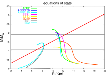
Figure 1: NS mass versus radius for the models of EOS described in the text. The two horizontal lines denote the boundaries of the region of observationally allowed NS masses, while the red straight line corresponds to the mass-radius relation extracted from the redshift measurement of Cottam et al. (2002)

In Table II we give the parameters of the stellar models for which we shall compute the frequencies of the QNM. For each EOS we tabulate the central density in $g/cm^{3}$, the stellar radius in km and the compactness $M/R$ ($M$ and $R$ in km), for assigned values of the gravitational mass, that range from $1.2~{}M_{\odot}$ to the maximum mass given in Table I. Empty slots correspond to values of the mass which exceed the maximum mass of the considered EOS.

III The quasi-normal mode frequencies

To find the frequencies and damping times of the quasi-normal modes we solve the equations describing the non radial perturbations of a non rotating star in general relativity. These equations are derived by expanding the perturbed tensors in tensorial spherical harmonics in an appropriate gauge, closing the system with the selected EOS. The perturbed equations split into two distinct sets, the axial and the polar which belong, respectively, to the harmonics that transform like  $(-1)^{(\ell+1)}$  and  $(-1)^{(\ell)}$  under the parity transformation  $\theta\rightarrow\pi-\theta$  and  $\varphi\rightarrow\pi+\varphi.$  A quasi-normal mode of the star is defined to be a solution of the perturbed equations belonging to complex eigenfrequency, which is regular at the center and continuous at the surface, and which behaves as a pure outgoing wave at infinity. The real part of the frequency is the pulsation frequency, the imaginary part is the inverse of the damping time of the mode due to gravitational wave emission. It is customary to classify the QNM according to the source of the restoring force which prevails in bringing the perturbed element of fluid back to the equilibrium position. Thus, we have a g-mode if the restoring force is mainly provided by buoyancy or a p-mode if it is due to a gradient of pressure. The frequencies of the g-modes are lower than those of the p-modes, the two sets being separated by the frequency of the fundamental mode, which is related to the global oscillations of the fluid. In general relativity there exist further modes that are purely gravitational since they do not induce fluid motion, named w-modes CF1991 ; KS1992 . The w-modes are both polar and axial, they are highly damped and, in general, their frequencies are higher than the p-mode frequencies, apart from a branch, named w_II, for which the frequencies are comparable to those of the p-modes.

We integrate the perturbed equations in the frequency domain. For the polar ones, we integrate the set of equations used in tutti4 ; for each assigned value of the harmonic index $~{}l~{}$ and of the frequency $~{}\nu~{}$, they admit only two linearly independent solutions regular at $~{}r=0$. The general solution is found as a linear combination of the two, such that the Lagrangian perturbation of the pressure vanishes at the surface. Outside the star, the solution is continued by integrating the Zerilli equation to which the polar equations reduce when the fluid perturbations vanish zerilli . For the axial perturbations we integrate the Schrödinger-like equation derived in CF1990 .

To explicitely compute the QNM eigenfrequencies we follow two different procedures: for the slowly damped modes i.e. those, as the f- and p-modes, for which the imaginary part of the frequency is much smaller than the real part we use the algorithm developed in CF1990 ; CFW1991 : the perturbed equations are integrated for real values of the frequency from $r=0$ to radial infinity, where the amplitude of the Zerilli function is computed; the frequency of a QNM can be shown to correspond to a local minimum of this function and the damping time is given in terms of the width of the parabola which fits the wave amplitude as a function of the frequency near the minimum. We shall indicate this method as the CF-algorithm.

For highly damped modes, when the imaginary part of the frequency is comparable to (or greather than) the real part, the CF-algorithm cannot be applied and we use the continued fractions method LNS , integrating the perturbed equations in the complex frequency domain. With this method we find the frequencies of the axial and polar w-modes. A clear account on continued fractions can be found in STM . However, it should be mentioned that this algorithm cannot be applied when $M/R\geq 0.25$, and therefore the w-mode frequencies cannot be computed for ultracompact stars.

The results of the numerical integration for $l=2$ are summarized in Table III and IV. Table III refers to the polar quasi-normal modes; the frequency and the damping time of the f-mode, of the first p-mode and of the first polar w- and w_II-mode are given for the stellar models of Table II. In Table IV we give the frequency and the damping time of the the first axial w- and w_II-mode for the same stellar models. In Table III and IV there are some empty slots for the w- and w_II-modes: they refer to stellar models having $M/R\geq 0.25$ for which neither the CF-algorithm nor the continued fractions method can be applied.

		$1.2~{}M_{\odot}$	$1.4~{}M_{\odot}$	$1.5~{}M_{\odot}$	$1.8~{}M_{\odot}$	$2~{}M_{\odot}$	$~{}M_{max}$
	$\rho_{c}/\rho_{0}$	0.735	0.815	0.859	1.016	1.163	2.357
APR1	R (km)	12.31	12.28	12.26	12.15	12.00	10.77
	M/R	0.144	0.168	0.181	0.219	0.246	0.326
	$\rho_{c}/\rho_{0}$	0.884	0.994	1.056	1.294	1.562	2.794
APR2	R (km)	11.66	11.58	11.53	11.31	11.03	10.03
	M/R	0.152	0.179	0.192	0.235	0.268	0.325
	$\rho_{c}/\rho_{0}$	0.890	0.996	1.056	1.285	1.795	2.457
APRB200	R (km)	11.50	11.45	11.42	11.24	10.92	10.73
	M/R	0.154	0.181	0.194	0.236	0.270	0.279
	$\rho_{c}/\rho_{0}$	0.890	0.997	1.080	1.540	–	2.516
APRB120	R (km)	11.50	11.45	11.42	11.08	–	10.60
	M/R	0.154	0.181	0.194	0.240	–	0.264
	$\rho_{c}/\rho_{0}$	0.766	0.888	0.960	1.289	2.061	2.509
BBS1	R (km)	12.39	12.96	12.19	11.80	11.03	10.70
	M/R	0.143	0.169	0.182	0.225	0.268	0.279
	$\rho_{c}/\rho_{0}$	1.811	–	–	–	–	2.666
BBS2	R (km)	11.18	–	–	–	–	10.43
	M/R	0.159	–	–	–	–	0.172
	$\rho_{c}/\rho_{0}$	0.712	1.070	1.525	–	–	2.565
G240	R (km)	13.55	12.92	12.20	–	–	11.00
	M/R	0.131	0.160	0.182	–	–	0.208
	$\rho_{c}/\rho_{0}$	1.638	2.448	–	–	–	3.771
SS1	R (km)	9.02	8.83	–	–	–	8.42
	M/R	0.197	0.234	–	–	–	0.255
	$\rho_{c}/\rho_{0}$	1.641	2.453	–	–	–	3.777
SS2	R (km)	8.17	8.20	–	–	–	7.91
	M/R	0.217	0.252	–	–	–	0.271

Table 2: Parameters of the considered stellar models: for each EOS and for each assigned value of the stellar mass, we give the central density $\rho_{c}$ in units of $\rho_{0}=10^{15}$ g/cm³, the radius $R$ in km and the compactness $M/R$ ($M$ and $R$ in km). Empty slots refer to masses that exceed the maximum mass.

M	EOS	$\nu_{f}$ (Hz)	$\tau_{f}$ (ms)	$\nu_{p_{1}}$ (Hz)	$\tau_{p_{1}}$ (s)	$\nu_{w_{1}}$ (Hz)	$\tau_{w_{1}}$ ($\mu$s)	$\nu_{w_{1}^{\!I\!I\!}}$ (Hz)	$\tau_{w_{1}^{\!I\!I\!}}$ ($\mu$s)
$1.2~{}M_{\odot}$	APR1	1737	278	5648	6.5	12023	19.3	5029	18.8
	APR2	1886	234	5825	4.9	12378	19.2	5493	18.3
	APRB200	1906	229	6076	5.5	12465	19.2	5565	18.3
	APRB120	1906	229	6079	5.5	12466	19.2	5566	18.3
	BBS1	1726	281	5648	5.6	11961	19.4	4983	18.9
	BBS2	2090	193	5626	1.0	12450	19.7	6002	17.6
	G240	1545	356	4897	4.7	11332	19.8	4398	19.6
	SS1	2526	134	10566	26.2	13747	19.7	7669	17.1
	SS2	2529	134	11247	21.2	13758	19.7	7682	17.1
$1.4~{}M_{\odot}$	APR1	1818	216	5922	5.8	11092	22.4	5366	18.8
	APR2	1983	184	6164	4.4	11360	22.5	5906	20.2
	APRB200	1997	181	6410	5.1	11407	22.6	5962	20.2
	APRB120	1998	181	6413	5.0	11405	22.6	5963	20.2
	BBS1	1832	213	5861	4.2	11066	22.5	5394	20.6
	G240	1763	231	5055	1.9	10737	22.8	5100	20.7
	SS1	2736	109	9428	4.2	11919	26.4	8594	18.8
	SS2	2739	109	9467	4.4	–	–	–	–
$1.5~{}M_{\odot}$	APR1	1856	195	6045	5.6	10635	24.2	5538	21.6
	APR2	2030	167	6320	4.3	10845	24.6	6125	21.2
	APRB200	2041	165	6557	4.9	10879	24.6	6172	21.1
	APRB120	2042	165	6501	4.9	10879	24.6	6174	21.1
	BBS1	1887	190	5953	3.7	10621	24.3	5618	21.5
	G240	1984	175	5176	1.0	10484	25.3	5831	20.8
$1.8~{}M_{\odot}$	APR1	1969	156	6355	5.8	9246	31.5	6213	24.56
	APR2	2171	137	6708	5.1	9240	34.3	6876	24.0
	APRB200	2174	136	6902	6.1	9248	34.3	6896	24.0
	APRB120	2229	132	6887	3.8	9223	35.8	7067	23.8
	BBS1	2076	145	6178	2.9	9205	33.2	6472	24.1
$2~{}M_{\odot}$	APR1	2047	144	6498	7.9	8303	40.5	6548	26.4
	APR2	2280	132	6876	12.0	–	–	–	–
	APRB200	2300	131	7031	11.3	–	–	–	–
	BBS1	2326	131	6286	2.6	–	–	–	–
$M_{max}$	APR1	2349	186	6384	0.36	–	–	–	–
	APR2	2537	172	6808	0.38	–	–	–	–
	APRB200	2361	132	7013	9.7	–	–	–	–
	APRB120	2401	125	6850	2.4	–	–	–	–
	BBS1	2423	131	6297	2.5	–	–	–	–
	BBS2	2365	153	5790	0.51	12639	20.7	6844	16.9
	G240	2357	133	5460	0.49	10425	30.0	7091	20.0
	SS1	2978	99	8644	1.5	–	–	–	–
	SS2	2990	99	8661	1.5	–	–	–	–

Table 3: The frequencies and the damping times of the polar QNM for $l=2$ are tabulated for assigned values of the stellar mass and for the considered EOS’s. For stellar models having $M/R\geq 0.25$ (cfr. Table II) the w-mode frequency can be computed neither using the CF-algorithm nor by the continued fraction method, and the corresponding slot is left empty.

M	EOS	$\nu_{w_{1}}$ (Hz)	$\tau_{w_{1}}$ ($\mu$s)	$\nu_{w_{1}^{\!I\!I\!}}$ (Hz)	$\tau_{w_{1}^{\!I\!I\!}}$ ($\mu$s)
$1.2~{}M_{\odot}$	APR1	8029	24.6	1626	12.7
	APR2	8437	24.6	2081	12.3
	APRB200	8496	24.6	2162	12.2
	APRB120	8496	24.6	2162	12.2
	BBS1	7989	24.5	1580	12.8
	BBS2	8925	24.4	2545	11.8
	G240	7442	24.6	1019	13.5
	SS1	9990	26.1	4498	10.9
	SS2	9997	26.1	4520	10.8
$1.4~{}M_{\odot}$	APR1	7757	29.0	2476	13.6
	APR2	8156	29.5	3040	13.1
	APRB200	8190	29.5	3110	13.1
	APRB120	8189	29.6	3110	13.1
	BBS1	7785	29.0	2495	13.6
	G240	7588	28.6	2157	13.9
	SS1	9655	34.5	6050	11.09
	SS2	–	–	–	–
$1.5~{}M_{\odot}$	APR1	7625	31.6	2875	14.0
	APR2	8016	32.4	3499	13.6
	APRB200	8040	32.5	3559	13.5
	APRB120	8042	32.5	3562	13.5
	BBS1	7691	31.7	2947	14.0
	G240	7910	31.7	3105	13.6
$1.8~{}M_{\odot}$	APR1	7236	41.9	4028	15.5
	APR2	7590	45.2	4865	15.2
	APRB200	7593	43.3	4894	15.2
	APRB120	7683	46.3	5096	15.1
	BBS1	7436	43.3	4399	15.3
$2~{}M_{\odot}$	APR1	6973	52.8	4896	16.9
	APR2	–	–	–	–
	APRB200	–	–	–	–
	BBS1	–	–	–	–
$M_{max}$	APR1	–	–	–	–
	APR2	–	–	–	–
	APRB200	–	–	–	–
	APRB120	–	–	–	–
	BBS1	–	–	–	–
	BBS2	–	–	–	–
	BBS2	9567	25.3	3436	11.4
	G240	8616	36.2	4562	13.3
	SS1	–	–	–	–
	SS2	–	–	–	–

Table 4: The frequencies and the damping times of the axial QNM for $l=2$ are tabulated for assigned values of the stellar mass and for the considered EOS’s. As in Table III, when the mode frequency cannot be computed the slot is left empty.

III.1 Fits and Plots

As done in ref.AK , the data of Tables III and IV can be fitted by suitable functions of the mass and of the radius of the NS. We exclude from the fit the data which refer to the equation of state APR1, since we include APR2 which is an improved version of APR1; we also exclude the data referring to strange stars, because there is a very large degree of arbitrariness in the choice of the bag model parameters; conversely, the EOS from which we derive the empirical relations fit at least some (or many) experimental data on nuclear properties and nucleon-nucleon scattering and/or some observational data on NSs. However, in all figures we shall also plot the data corresponding to APR1 and to strange stars for comparison.

In refs.AK and AK1 it was shown how the fits should be used to set stringent constraints on the mass and radius of the star provided the frequency and the damping times of some of the modes are detected in a gravitational signal, and we shall not repeat the analysis here. We shall rather focus on a different aspect of the problem showing that, if we know the mass of the star, the QNM frequencies can be used to gain direct information on the EOS of nuclear matter, and to this purpose we shall plot the mode frequencies as a function of the stellar mass.

Let us consider the fundamental mode firstly. Numerical simulations show that this is the mode which is mostly excited in many astrophysical processes and consequently the major contribution to gravitational wave emission should be expected at this frequency. Moreover, as for the p-modes, its damping time is quite long compared to that of the w-modes, therefore it should appear in the spectrum of the gravitational signal as a sharp peak and should be easily identifiable.

It is known from the Newtonian theory of stellar perturbations that the f-mode frequency scales as the square root of the average density; thus, the data given in Table III can be fitted by the following expression

$$\nu_{f}=a+b\sqrt{\frac{M}{R^{3}}},\quad a=0.79\pm 0.09,\quad b=33\pm 2,$$ (2)

where $a$ is given in kHz and $b$ in km $\cdot$ kHz. In this fit and hereafter in all fits, frequencies will be expressed in kHz, masses and radii in km, damping times in s and $c=3\cdot 10^{5}$km/s.

In a similar way, the damping time of the f-mode can be fitted as a function of the compactness $M/R$ as follows

$$\tau_{f}=\frac{R^{4}}{cM^{3}}\left[a+b\frac{M}{R}\right]^{-1}\,,$$ (3)

$$a=[8.7\pm 0.2]\cdot 10^{-2},\qquad b=-0.271\pm 0.009\,.$$

The data for the f-mode and the fits are shown in Fig. 2. In the upper panel we plot $\nu_{f}$ versus $M/R^{3}$, for all stellar models considered in Table III. The fit (2) is plotted as a dashed line, and the fit given in AK , which is based on the EOSs considered in that paper, is plotted as a continuous line labelled as ‘AK-fit’. In the lower panel we plot the damping time $\tau_{f}$ versus the compactness $M/R$, our fit and the corresponding AK-fit.

From Fig. 2 we see that our new fit for $\nu_{f}$ is sistematically lower than the AK fit by about 100 Hz; this basically shows that the new EOS are, on average, less compressible (i.e. stiffer) than the old ones. Conversely, eq. (3) is very similar to the fit found in AK .

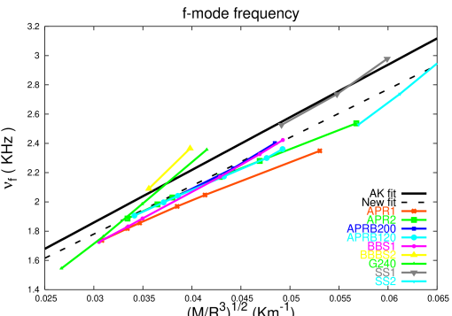
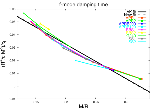
Figure 2: The frequency of the fundamental mode is plotted in the upper panel as a function of the square root of the average density for the different EOS considered in this paper. We also plot the fit given by Andersson and Kokkotas (AK-fit) and our fit (New fit). The new fit is systematically lower (about 100 Hz) than the old one. The damping time of the fundamental mode is plotted in the lower panel as a function of the compactness $M/R$. The AK-fit and our fit, plotted respectively as a continuous and a dashed line, do not show significant differences.

The frequency of the first p-mode can be fitted as a function of the compactness

$$\nu_{p_{1}}=\frac{1}{M}\left[a+b\frac{M}{R}\right],\qquad a=-1.5\pm 0.8,\quad b=79\pm 4,$$ (4)

where $a$ and $b$ are given in km$\cdot$kHz, whereas, as already noted in AK , the damping times are so spread out that a fit has no significance.

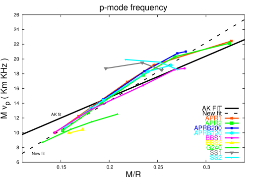
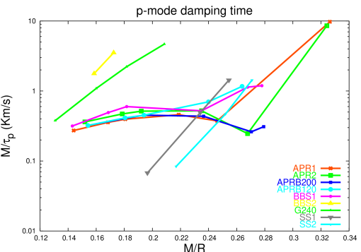
Figure 3: The frequency (upper panel) and the damping time (lower panel) of the first p-mode are plotted as a function of the compactness of the star. The AK-fit and the new fit for the frequency are plotted, in the upper panel, as a continuous and dashed line, respectively. As already noted in (AK) the data referring to the damping time are so spread that a fit has no significance.

The data for the mode ${p_{1}}$ are shown in Fig. 3. In the upper panel we plot $\nu_{p_{1}}$ multiplied by the stellar mass M, the new fit and the corresponding AK-fit, versus the star compactness; it can be noted that the two fits have a different slope. In the lower panel the inverse of the damping time multiplied by the mass ($M/\tau_{p}$) is plotted versus $M/R$: the spread of the data is apparent.

The frequencies and damping times of the first polar and the axial $w$-modes are very well fitted by suitable functions of the compactness as follows

$$\nu_{w_{1}}^{pol}=\frac{1}{R}\left[a+b\frac{M}{R}\right]\,,$$ (5)

$$a=215.5\pm 1.3\quad b=-474\pm 7,$$

where $a$ and $b$ are given in km $\cdot$ kHz,

$$\tau_{w_{1}}^{pol}=10^{-3}\cdot M\left[a+b\frac{M}{R}+d\left(\frac{M}{R}\right)^{2}\right]^{-1}\,,$$ (6)

$$a=36\pm 19\quad b=720\pm 200,\quad d=-2300\pm 500,$$

where $a$, $b$ and $d$ are given in km/s,

$$\nu_{w_{1}^{II}}^{pol}=\frac{1}{M}\left[a+b{\frac{M}{R}}\right]\,$$ (7)

$$a=-5.8\pm 0.4\quad b=102\pm 2\,,$$

where $a$ and $b$ are given in km $\cdot$ kHz,

$$\tau_{w_{1}^{II}}^{pol}=10^{-3}\cdot M\left[a+b\frac{M}{R}+d\left(\frac{M}{R}\right)^{2}\right]^{-1}\,,$$ (8)

$$a=21\pm 16\quad b=700\pm 170,\quad d=-1400\pm 500\,,$$

$a$, $b$ and $d$ are given in km/s;

$$\nu_{w_{1}}^{ax}=\frac{1}{R}\left[a+b{\frac{M}{R}}\right]\,,$$ (9)

$$a=121\pm 2\quad b=-146\pm 12\,,$$

where $a$ and $b$ are given in km $\cdot$ kHz,

$$\tau_{w_{1}}^{ax}=10^{-3}\cdot M\left[a+b\frac{M}{R}+d\left(\frac{M}{R}\right)^{2}\right]^{-1}\,,$$ (10)

$$a=48\pm 6\quad b=360\pm 70,\quad d=-1340\pm 170,$$

where $a$, $b$ and $d$ are given in km/s,

$$\nu_{w_{1}^{II}}^{ax}=\frac{1}{M}\left[a+b{\frac{M}{R}}\right]\,,$$ (11)

$$a=-13.1\pm 0.4\quad b=110\pm 2\,,$$

where $a$ and $b$ are given in km $\cdot$ kHz,

$$\tau_{w_{1}^{II}}^{ax}=10^{-3}\cdot M\left[a+b\frac{M}{R}+d\left(\frac{M}{R}\right)^{2}\right]^{-1}\,,$$ (12)

$$a=-7\pm 11\quad b=1400\pm 120,\quad d=-2700\pm 300,$$

where $a$, $b$ and $d$ are given in km/s. We do not plot all fits and data for the w-modes because the graphs would not add more relevant information.

The empirical relations derived above could be used, as described in AK ; AK1 , to determine the mass and the radius of the star from the knowledge of the frequency and damping time of the modes; but now we want to address a different question: we want to understand whether the knowledge of the mode frequencies and of the mass of the star, which is after all the only observable on which we might have reliable information, can help in discriminating among the different EOSs. To this purpose in Fig. 4 we plot $\nu_{f}$, as a function of the mass, for all EOS and all stellar models given in Table III.

Comparing the values of $\nu_{f}$ for APR1 and APR2 we immediately see that the relativistic corrections and the associated redefinition of the three-body potential, which improve the Hamiltonian of APR2 with respect to APR1 , play a relevant role, leading to a systematic difference of about 150 Hz in the mode frequency. Conversely, the presence of quark matter in the star inner core (EOS ${\rm APRB200~{}}$ and ${\rm APRB120~{}}$) does not seem to significantly affect the pulsation properties of the star. This is a generic feature, which we observe also in the p- and w- modes behavior.

From Fig. 4 we also see that the frequencies corresponding to the BBS1 and APR1 models, which are very close at $M\mathrel{\hbox to0.0pt{\lower 2.5pt\hbox{\hskip 1.0pt$\sim$}\hss}\raise 1.0pt\hbox{$<$}}1.4$, diverge for larger masses. This behavior is to be ascribed to the different treatments of three-nucleon interactions, whose role in shaping the EOS becomes more and more important as the star mass (and central density) increases: while the variational approach of ref. AP used to derive the EOS APR1 naturally allows for inclusion of the three-nucleon potential appearing in Eq.(1), in G-matrix perturbation theory used to derive the EOS BBS1 , $V_{ijk}$ has to be replaced with an effective two-nucleon potential ${\widetilde{V}}_{ij}$, obtained by averaging over the position of the third particle lejeune .

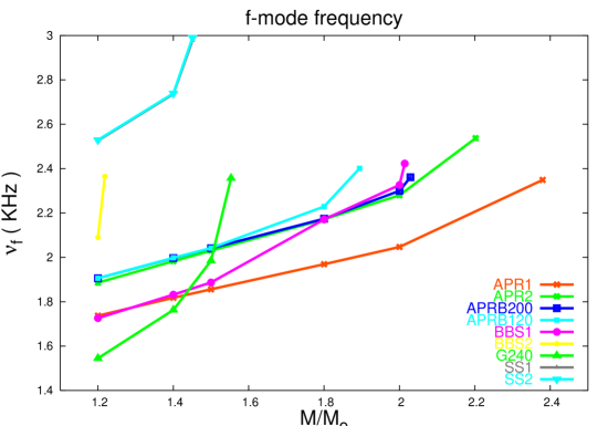
Figure 4: The frequency of the fundamental mode is plotted as a function of the mass of the star.

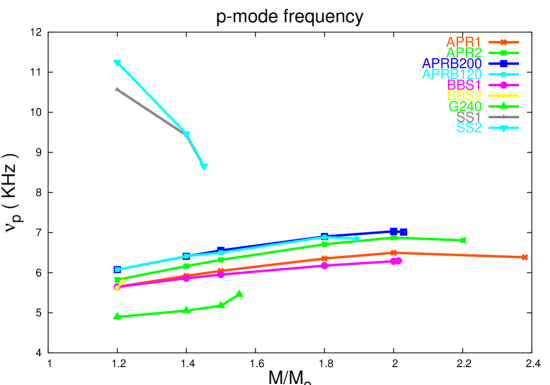
Figure 5: The frequency of the first p-mode is plotted as a function of the mass of the star.

The transition to hyperonic matter, predicted by the BBS2 model, produces a sizable softening of the EOS, thus leading to stable NS configurations of very low mass. As a consequence of the softening of the EOS, the corresponding f-mode frequency is significantly higher than those obtained with the other EOS. So much higher, in fact, that its detection would provide evidence of the presence of hyperons in the NS core.

It is also interesting to compare the f-mode frequencies corresponding to models BBS2 and G240 , as they both predict the occurrence of heavy strange baryons but are obtained from different theoretical approaches, based on different descriptions of the underlying dynamics. The behavior of $\nu_{f}$ displayed in Fig. 4 directly reflects the relations between mass and central density obtained from the two EOS, larger frequencies being always associated with larger densities. For example, the NS configurations of mass $\sim$ 1.2 $M_{\odot}$ obtained from the G240 and BBS2 have central densities $\sim$ 7$\cdot$10¹⁴ g/cm³ and $\sim$ 2.5$\cdot$10¹⁵ g/cm³, respectively. On the other hand, the G240 model requires a central density of $\sim$ 2.5$\cdot$10¹⁵ g/cm³ to reach a mass of $\sim$ 1.55 $M_{\odot}$ and a consequent $\nu_{f}$ equal to that of the BBS2 model.

Strange stars models, SS1 and SS2 also correspond to values of $\nu_{f}$ well above those obtained from the other models. The peculiar properties of these stars, which are also apparent from the mass-radius relation shown in Fig. 1 largely depend upon the self-bound nature of strange quark matter.

IV Concluding Remarks

Having shown how the internal structure affects the frequencies at which a neutron star oscillates and emit gravitational waves, it is interesting to ask whether the present generation of gravitational antennas may actually detect these signals. To this purpose, let us consider, as an example, a neutron star with an inner core composed of nuclear matter satisfying the EOS APR2 . Be $M=1.4~{}M_{\odot}$ its mass, and let us assume that its fundamental mode has been excited by some external or internal event ($\nu_{f}=1983~{}Hz$, $\tau_{f}=0.184~{}s$, see Table III). The signal emitted by the star can be modeled as a damped sinusoid Kyoto2002

$$h(t)={\cal{A}}e^{(t_{\rm arr}-t)/\tau_{f}}\sin\left[2\pi\nu_{f}\left(t-t_{\rm arr}\right)\right]\ ,$$ (13)

where $t_{\rm arr}$ is the arrival time and ${\cal A}$ is the mode amplitude; the energy stored into the mode can be estimated by integrating over the surface and over the frequency the expression of the energy flux

$$\frac{dE_{\rm{mode}}}{dSd\nu}=\frac{\pi}{2}\,\nu^{2}\,|\,\tilde{h}(\nu)\,|^{2},$$ (14)

where $h(\nu)$ is the Fourier-transorm of $h(t)$. Would we be able to detect this signal with, say, the ground based interferometric antenna VIRGO?

The VIRGO noise power spectral density can be modeled as DIS1

$$S_{n}(x)=10^{-46}\cdot\left\{3.24[(6.23x)^{-5}+2x^{-1}+1+x^{2}]\right\}~{}Hz^{-1},$$ (15)

where $x=\nu/\nu_{0}$, with $\nu_{0}=500~{}Hz$; at frequencies lower than the cutoff frequency $\nu_{s}=20~{}Hz$ the noise sharply increases. Assuming that we extract the signal from noise by using the optimal matched filtering technique, the signal to noise ratio (SNR) can easily be computed from the following expression

$$SNR=2\left[\int_{0}^{\infty}~{}d\nu~{}\frac{|\tilde{h}(\nu)|^{2}}{S_{n}(\nu)}\right]^{1/2}.$$ (16)

Using eqs. (13-16) we find that in order to reach SNR=5, which is good enough to garantee detection, the energy stored into the f-mode should be $E_{f-mode}\sim 6\cdot 10^{-7}~{}M_{\odot}c^{2}$ for a source in our Galaxy (distance from Earth $d\sim 10~{}kpc$) and $E_{f-mode}\sim 1.3~{}M_{\odot}c^{2}$ for a source in the VIRGO cluster ($d\sim 15~{}Mpc$). Similar estimates can be found for the detectors LIGO, GEO, TAMA.

These numbers indicate that it is unlikely that the first generation of interferometric antennas will detect the gravitational waves emitted by an oscillating neutron star. However, new detectors are under investigation that should be much more sensitive at frequencies above 1-2 kHz and that whould be more appropriate to detect these signals.

If the frequencies of the modes will be identified in a detected signal, the simultaneous knowledge of the mass of the emitting star will be crucial to understand its internal composition. Indeed, as shown in Figs. 4 and 5, we would be able for instance to infer, or exclude, the presence of barions in the inner core, and to see whether nature allows for the formation of bare strange stars. We remark that in particular the f-mode and the first p-modes, that numerical simulations indicate as those that are most likely to be excited allenetal ; tutti2 , have relatively long damping times, and therefore their excitation should appear in the spectrum as a sharp peak at the corresponding frequency, a feature that would facilitate their identification.

References

- (1) L. Lindblom, S. Detweiler, Ap. J. Suppl. 53, 73, (1983)
- (2) N. Andersson, K.D. Kokkotas, MNRAS 299, 1059, (1998)
- (3) R.B. Wiringa, V. Fiks, A. Fabrocini, Phys. Rev. C 38, 1010, (1988)
- (4) O. Benhar, E. Berti, V. Ferrari, MNRAS 310, 797, (1999).
- (5) G. Baym, C.J. Pethick, P. Sutherland, Ap. J. 170, 299, (1971)
- (6) C.J. Pethick, B.G. Ravenhall, C.P. Lorenz, Nucl. Phys. A584, 675, (1995)
- (7) R.B. Wiringa, V.G.J. Stoks, R. Schiavilla, Phys. Rev. C 51, 38, (1995)
- (8) B.S. Pudliner, V.R. Pandharipande, J. Carlson, S.C. Pieper, R.B. Wiringa, Phys. Rev. C 56, 1720, (1995)
- (9) S.C. Pieper and R.B. Wiringa, Ann. Rev. Nucl. Part. Sci. 51 (2001) 53
- (10) A. Akmal, V. R. Pandharipande, Phys. Rev. C 56, 2261 , (1997)
- (11) M. Baldo, G. Giansiracusa, U. Lombardo, H.Q. Song, Phys. Lett. B473, 1, (2000)
- (12) J.D. Walecka, Ann. Phys. 83, 491, (1974)
- (13) P.M.M. Maessen, T.A. Rijken, J.J. deSwart, Phys. Rev. C 40, 2226, (1989)
- (14) L.P. Kadanoff, G. Baym, Quantum Statistical Mechanics (Benjamin, New York, 1972)
- (15) A. Chodos, R.L. Jaffe, K. Johnson, C.B. Tohm, V.F. Weisskopf, Phys. Rev. D, 9, 3471, (1974)
- (16) A. Akmal, V. R. Pandharipande, D.G. Ravenhall Phys. Rev. C 58, 1804 , (1998)
- (17) R. Rubino, thesis, Università “La Sapienza”, Roma (unpublished); O. Benhar, R. Rubino, to be published.
- (18) M. Baldo, G.F. Burgio, H.J. Schulze, Phys. Rev. C, 61, 055801, (2000)
- (19) N.K. Glendenning, Compact Stars (Springer, New York, 2000)
- (20) A.R. Bodmer, Phys. Rev. D, 4, 1601, (1971)
- (21) E. Witten, Phys.Rev. 30, 272, (1984)
- (22) S.E. Thorsett, D. Chakrabarty, Ap. J. , 512, 288, (1999)
- (23) H. Quaintrell, et al., Astron. Astrophys., 401, 303, (2003)
- (24) J. Cottam et al, Nature, 420, 51, (2002)
- (25) M. Dey, I. Bombaci, J. Dey, R. Subharthi, B.C. Samanta, Phys. Lett. B438, 123, (1999)
- (26) S. Chandrasekhar, V. Ferrari, Proc. R. Soc. Lond. A434, 449, (1991)
- (27) K.D. Kokkotas, B.F. Schutz, MNRAS, 255, 119 (1992)
- (28) G. Miniutti, J.A. Pons, E. Berti, L. Gualtieri and V. Ferrari, MNRAS, 338, 389 , (2003)
- (29) J.F. Zerilli, Phys. Rev D 2, 2141 , (1970)
- (30) S. Chandrasekhar, V. Ferrari, Proc. R. Soc. Lond. A432, 247, (1990)
- (31) S. Chandrasekhar, V. Ferrari, R. Winston, Proc. R. Soc. Lond. A434, 635, (1990)
- (32) M. Leins, H.P. Nollert, M.H. Soffel, Phys.Rev. D 48, 3467, (1993)
- (33) H. Sotani, K. Tominaga, K.I. Maeda, Phys. Rev. D65, 024010, (2001)
- (34) N. Andersson, K.D. Kokkotas, MNRAS 320, 307, (1999)
- (35) A. Lejeune, P. Grangé, P. Martzoff and J. Cugnon, Nucl. Phys. A453, 189, (1986)
- (36) V. Ferrari, G. Miniutti, J. A. Pons, Class. Quant. Grav., 20, 8841, (2003).
- (37) T. Damour, B. R. Iyer, B. S. Sathyaprakash, Phys. Rev. D 57, 885, (1998).
- (38) G. Allen, N. Andersson, K.D. Kokkotas, B.F. Schutz, Phys. Rev. D58, 124012, (1998).
- (39) J.A. Pons, E. Berti, L. Gualtieri, G. Miniutti and V. Ferrari, Phys. Rev. D65, 104021, (2002).