Neutrinos from microquasars

Abstract

The jets of microquasars with high-mass stellar companions are exposed to the dense matter field of the stellar wind as well as to the photon densities found in the surrounding medium. Photopion and proton-proton interactions could then lead to copious production of neutrinos. In this work, we analyze the hadronic microquasar model, particularly in what concerns to the neutrino production. Limits to this kind of models using data from AMANDA-II are established. New constraints are also imposed upon specific microquasar models based on photopion processes. These are very restrictive particularly for the case of SS433, a microquasar for which the presence of accelerated hadrons has been already inferred from iron X-ray line observations.

1 Introduction

The presence of relativistic hadrons in microquasar jets like those of SS433 has been already inferred from iron X-ray line observations (e.g. Migliari et al. 2002). A significant content of relativistic hadrons in microquasar jets could open the possibility for a hadronically-generated emission of high energy radiation. Here, we discuss a new mechanism for the generation of high-energy gamma-rays in microquasars that is based on hadronic interactions occurring outside the coronal region (Romero et al. 2004). In this model the gamma-ray and neutrino emission arises from the decay of neutral pions created in the inelastic collisions between relativistic protons ejected by the compact object and ions in the stellar wind. The only requisites for the model to operate are a windy high-mass stellar companion and the presence of multi-TeV protons in the jet, both of which seem natural in microquasar environments. We pay particular attention to the possible neutrino signal of this kind of models, and impose constraints using the latest AMANDA-II data (Ahrens et al. 2004).

2 The hadronic microquasar model

2.1 The jet and the particle spectrum in the lab frame

For simplicity, we shall not make any specific assumption about the magnetic field or other parameters in the jet, but rather model it as a beam of energetic particles (i.e., in the spirit of, for instance, Purmohammad and Samimi 2001, and Bednarek et al. 1990). The jet axis, $z$, is assumed normal to the orbital radius $a$. We shall allow the jet to expand laterally, in such a way that its radius is given by $R(z)=\xi z^{\epsilon}$, with $\epsilon\leq 1$ and $z_{0}\leq z\leq z_{\rm max}$. For $\epsilon=1$ we have a conical beam. The jet starts to expand at a height $z_{0}\sim$ a few hundred km above the black hole, outside the coronal region. The particle spectrum of the relativistic $e-p$ flow is assumed to be a power law $N^{\prime}_{e,\;p}(E^{\prime}_{e,\;p})=K_{e,\;p}\;{E^{\prime}}_{e,\;p}^{-\alpha}$, valid for ${E^{\prime}_{e,\;p}}^{\rm min}\leq E^{\prime}_{e,\;p}\leq{E^{\prime}_{e,\;p}}^{\rm max}$, in the jet frame. The corresponding particle flux will be $J^{\prime}_{e,\;p}(E^{\prime}_{e,\;p})=(c/4\pi)N^{\prime}_{e,\;p}(E^{\prime}_{e,\;p})$. Since the jet expands, the proton flux can be written as:

$$J^{\prime}_{p}(E^{\prime}_{p})=\frac{c}{4\pi}K_{0}\left(\frac{z_{0}}{z}\right)^{\epsilon n}{E^{\prime}_{p}}^{-\alpha},$$ (1)

where $n>0$ (a value $n=2$ corresponds to the conservation of the number of particles, see Ghisellini et al. 1985), and a prime refers to the jet frame. Note that these expressions are valid in the jet frame. Using relativistic invariants, it can be proven that the proton flux, in the observer (or lab) frame, becomes (e.g. Purmohammmad & Samimi 2001)

$$J_{p}(E_{p},\theta)=\frac{cK_{0}}{4\pi}\left(\frac{z_{0}}{z}\right)^{\epsilon n}\frac{\Gamma^{-\alpha+1}\left(E_{p}-\beta_{\rm b}\sqrt{E_{p}^{2}-m_{p}^{2}c^{4}}\cos\theta\right)^{-\alpha}}{\left[\sin^{2}\theta+\Gamma^{2}\left(\cos\theta-\frac{\beta_{\rm b}E_{p}}{\sqrt{E_{p}^{2}-m_{p}^{2}c^{4}}}\right)\right]^{1/2}},$$ (2)

where $\Gamma$ is the jet Lorentz factor, $\theta$ is the angle subtended by the emerging photon direction (assumed to be similar to the initial proton direction) and the jet axis, $\beta_{\rm b}$ is the corresponding velocity in units of $c$. Note that only photons emitted with angles similar to that of the inclination angle of the jet will reach a distant observer, and thus $\theta$ can be approximated by the jet inclination angle.

In order to obtain Eq. (2) one has to consider conservation of particles. If $n$ is the number of protons per unit energy per unit solid angle per unit volume, so that in the frame comoving with the jet one has $n^{\prime}(E^{\prime},\Omega^{\prime})=(A/4\pi)E^{\prime-\alpha}dV^{\prime}$, the equality $n(E,\Omega)dVd\Omega dE=n^{\prime}(E^{\prime},\Omega^{\prime})dV^{\prime}d\Omega^{\prime}dE^{\prime}$ holds, what implies $n(E,\Omega)=n^{\prime}(E^{\prime},\Omega^{\prime})(d\Omega^{\prime}/d\Omega)(dE^{\prime}/dE)(dV^{\prime}/dV)$. From the invariance of $d^{3}p/E$, the invariance of $pd\Omega dE$ is also proved (Hayakawa 1969, p.715), so that $(d\Omega/d\Omega^{\prime})(dE^{\prime}/dE)=p/p^{\prime}$. Using relativistic Lorentz transformations, $p_{\|}^{\prime}=\Gamma(p_{\|}+\beta E)$, with $p_{\|}=p\cos\theta$ and $p_{\perp}^{\prime}=p_{\perp}=p\sin\theta$, what implies $p^{\prime 2}=p^{2}(\sin^{2}\theta+\Gamma^{2}(\cos\theta+\beta E/\sqrt{E^{2}-m^{2}})^{2})$. This defines $p/p^{\prime}$, which, together with the equalities $dV^{\prime}/dV=\Gamma$ and $E^{\prime}=\Gamma(E-\beta\sqrt{E^{2}-m^{2}}\cos\theta)$, yields to Eq. (2).

We will adopt the jet-disk coupling hypothesis proposed by Falcke & Biermann (1995) and applied with success to AGNs, i.e. the total jet power scales with the accreting rate as $Q_{\rm j}=q_{\rm j}\dot{M}_{\rm disk}c^{2}$, with $q_{\rm j}=10^{-1}-10^{-3}$. The number density ${n_{0}}^{\prime}$ of particles flowing in the jet at $R_{0}=R(z_{0})$ is then given by $c\pi R_{0}^{2}{n_{0}}^{\prime}=Q_{\rm j}/m_{p}c^{2}$, where $m_{p}$ is the proton rest mass. This implies:

$${n_{0}}^{\prime}=\frac{q_{\rm j}\dot{M}_{\rm disk}}{\pi cR_{0}^{2}m_{p}}$$ (3)

Additionally, $n_{0}^{\prime}=\int^{{E^{\prime}}_{p}^{\rm max}}_{{E^{\prime}}_{p}^{\rm min}}{N^{\prime}}_{p}({E^{\prime}}_{p},\;z_{0})\;d{E_{p}}^{\prime}$. Then, if ${E^{\prime}}_{p}^{\rm max}>>{E^{\prime}}_{p}^{\rm min}$, which is always the case, we have

$$K_{0}={n_{0}}^{\prime}(\alpha-1)({E^{\prime}}_{p}^{\rm min})^{\alpha-1},$$ (4)

which gives the constant in the power-law spectrum at $z_{0}$. This completely defines the proton spectrum.

2.2 Simple wind modelling

The structure of the matter field in the wind will be determined essentially by the stellar mass loss rate and the continuity equation: $\dot{M_{*}}=4\pi r^{2}\rho(r)v(r)$, where $\rho$ is the density of the wind and $v$ is its velocity. Hence,

$$\rho(r)=\frac{\dot{M_{*}}}{4\pi r^{2}v(r)}.$$ (5)

The radial dependence of the wind velocity is given by (Lamers & Cassinelli 1999):

$$v(r)=v_{\infty}\left(1-\frac{r_{*}}{r}\right)^{\beta},$$ (6)

where $v_{\infty}$ is the terminal wind velocity, $r_{*}$ is the stellar radius, and the parameter $\beta$ is $\sim 1$ for massive stars. Hence, using the fact that $r^{2}=z^{2}+a^{2}$ and assuming a gas dominated by protons, we get the particle density of the medium along the jet axis:

$$n(z)=\frac{\dot{M_{*}}}{4\pi m_{p}v_{\infty}(z^{2}+a^{2})}\left(1-\frac{r_{*}}{\sqrt{z^{2}+a^{2}}}\right)^{-\beta}.$$ (7)

Typical mass loss rates and terminal wind velocities for O stars are of the order of $10^{-5}$ $\dot{M_{\sun}}$ yr^-1 and 2500 km s^-1, respectively (Lamers & Cassinelli 1999). This simple modelling for the wind was also used when analyzing the possible TeV emission from stellar systems (Romero & Torres 2003, Torres et al. 2004).

It is important to note that we are considering not that the beam interacts with the wind in a face-on collision, but instead, that the wind diffuses into the jet from the side. The wind penetration into the jet outflow depends on the parameter $\varpi\sim vR(z)/D$, where $v$ is the corresponding velocity of wind/beam in the direction of diffusion, $R(z)$ is the radius of the jet at a height $z$ above the compact object, and $D$ is the diffusion coefficient. $\varpi$ measures the ratio between the diffusive and the convective timescale of the particles. In the Bohm limit, with typical magnetic fields $B_{0}\sim 1-10$ G, $\varpi\leq 1$, and the wind matter penetrates the jet.

2.3 Gamma-ray and neutrino emission

The dominant $\pi$-producing channels in the hadronic interactions of the jet with the wind are ($E_{\rm th}\sim m_{\pi}c^{2}$):

$$p+p \rightarrow p+\pi^{0}\rightarrow p+2\gamma$$ (8)

$$p+p \rightarrow n+\pi^{+}\rightarrow p+e^{-}+\bar{\nu}_{e}+e^{+}+\nu_{e}+\nu_{\mu}+\bar{\nu}_{\mu}$$ (9)

$$p+p \rightarrow p+\pi^{+}+\pi^{-}$$ (10)

$$\rightarrow p+e^{+}+\nu_{e}++2\bar{\nu}_{\mu}+e^{-}+\bar{\nu}_{e}+2\nu_{\mu},$$

where all symbols have their usual meaning in particle physics. Processes (9) and (10) lead to in situ pair creation and neutrino production. The differential gamma-ray emissivity from $\pi^{0}$-decays is:

$$q_{\gamma}(E_{\gamma})=4\pi\sigma_{pp}(E_{p})\frac{2Z^{(\alpha)}_{p\rightarrow\pi^{0}}}{\alpha}\;J_{p}(E_{\gamma},\theta)\eta_{\rm A}.$$ (11)

Here, the parameter $\eta_{\rm A}$ takes into account the contribution from different nuclei in the wind and in the jet (for standard composition of cosmic rays and interstellar medium $\eta_{\rm A}=1.4-1.5$, Dermer 1986). $J_{p}(E_{\gamma})$ is the proton flux distribution evaluated at $E=E_{\gamma}$. The cross section $\sigma_{pp}(E_{p})$ for inelastic $p-p$ interactions at energy $E_{p}\approx 10E_{\gamma}$ can be represented above $E_{p}\approx 10$ GeV by $\sigma_{pp}(E_{p})\approx 30\times[0.95+0.06\log(E_{p}/{\rm GeV})]$ mb. Finally, $Z^{(\alpha)}_{p\rightarrow\pi^{0}}$ is the so-called spectrum-weighted moment of the inclusive cross-section. Its value for different spectral indices $\alpha$ is given, for instance, in Table A1 of Drury et al. (1994). Notice that $q_{\gamma}$ is expressed in ph s^-1 erg^-1 when we adopt CGS units.

The spectral gamma-ray intensity (photons per unit of time per unit of energy-band) is:

$$I_{\gamma}(E_{\gamma},\theta)=\int_{V}n(\vec{r^{\prime}})q_{\gamma}(\vec{r^{\prime}})d^{3}\vec{r^{\prime}},$$ (12)

where $V$ is the interaction volume. The spectral energy distribution is $L^{\pi^{0}}_{\gamma}(E_{\gamma},\theta)=E_{\gamma}^{2}I_{\gamma}(E_{\gamma},\theta)$ and using eqs. (2), (3), (4), (7), (11) and (12), we get:

$$L^{\pi^{0}}_{\gamma}(E_{\gamma},\theta)\approx\;\frac{q_{\rm j}z_{0}^{\epsilon(n-2)}Z^{(\alpha)}_{p\rightarrow\pi^{0}}}{2\pi m_{p}^{2}v_{\infty}}\;\frac{\alpha-1}{\alpha}\;({E^{\prime}}_{p}^{\rm min})^{\alpha-1}\times$$

$$\dot{M}_{*}\dot{M}_{\rm disk}\;\sigma_{pp}(10\;E_{\gamma})\;\frac{\Gamma^{-\alpha+1}\left(E_{\gamma}-\beta_{\rm b}\sqrt{E_{\gamma}^{2}-m_{p}^{2}c^{4}}\cos\theta\right)^{-\alpha}}{\left[\sin^{2}\theta+\Gamma^{2}\left(\cos\theta-\frac{\beta_{\rm b}E_{\gamma}}{\sqrt{E_{\gamma}^{2}-m_{p}^{2}c^{4}}}\right)\right]^{1/2}}$$

$$\int_{z_{0}}^{\infty}\frac{z^{\epsilon(2-n)}}{(z^{2}+a^{2})}\left(1-\frac{r_{*}}{\sqrt{z^{2}+a^{2}}}\right)^{-\beta}dz.$$ (13)

This expression gives approximately the $\pi^{0}$-decay gamma-ray luminosity for a windy microquasar at energies $E_{\gamma}>1$ GeV, in a given direction $\theta$ with respect to the jet axis. The neutrino spectrum roughly satisfies (e.g., Dar & Laor 1997): ${dF_{\nu}}/{dE_{\nu}}\simeq 0.7{dF_{\gamma}}/{dE_{\gamma}}.$

3 Discussion on neutrino upper limits

Upper limits imposed by AMANDA II (Ahrens et al. 2003) in known microquasars are typically $F<4\times 10^{-7}(E/{\rm GeV})^{-2}{\rm GeV}^{-1}{\rm cm}^{-2}{\rm s}^{-1}$. This upper limit and the theoretical expectation for the neutrino production, given assumptions on the free parameters of the system, allows already to put some constraints on the most favorable hadronic models. For instance, the model in which the distance is $D=5$ kpc or less, $q_{j}$=10^-2 or higher, the stellar mass loss rate is 10^-5 M_⊙ yr^-1 or higher, and the jet is inclined only 10 degrees or less, is already ruled out by neutrino astronomy. Note that this model maximizes the gamma-ray and neutrino emission, by enhancing the target matter density for proton interactions, by locating the microquasar at roughly half the distance to the Galactic Center, and by assuming a matter content in the jet with a significant dose of hadrons. In any case, this is a strong result in the sense that there is no need for any pointing of any telescope (the only assumption is that the microquasar is in the northern hemisphere, in the field of view of the AMANDA-II experiment). Note, however, that still there are plenty of models (different choices of system parameters) between the atmospheric neutrino background and the typically imposed upper limits; these have improved observational expectations for ICECUBE (as an example, models with proton slope 2.2 are shown in Figure 1).

Note that alternative hadronic microquasar models make use of photopion production of neutrinos (Levinson & Waxman 2001). The underlying idea in this kind of scenarios is that neutrinos are the result of photopion processes with synchrotron photons and external target fields surrounding the microquasar jet. Distefano et al. (2002), have presented the expectations for the neutrino fluxes from known microquasars under the assumed validity of this model, and focused on their scrutiny with the forthcoming ICECUBE neutrino telescope. Apart from a technical point –ICECUBE search bin is most likely going to be 1 degree, not 0.3, what would enhance the background significantly from Distefano et al. estimates, making detection more difficult– the strong claim in their study is that they predict in some cases even hundreds of events per year in a km-scale detector like ICECUBE. These would make of microquasars the most notable neutrino sources in the sky. For instance, in the case of SS433, the prediction is 252 muons events/yr above 1 TeV. But this implies around 20 or more events per year in AMANDA-II, what is ruled out already by data. Table 1 shows a comparison between the predictions of Distefano et al. (2002) and the measured upper limits extracted from the work of Ahrens et al. (2004), assuming a $E^{-2}$ spectrum, for some of the cases that appear to be already ruled out, or are on the verge of being ruled out, by AMANDA-II data. Note that the case of SS433 is especially significant: in this case it is known for sure that in the microquasar’s jets there are protons and heavy nuclei accelerated to relativistic speeds. For SS433, the estimations of Distefano et al. are ruled out by about one order of magnitude. Further analysis of neutrino upper limits will be presented elsewhere.

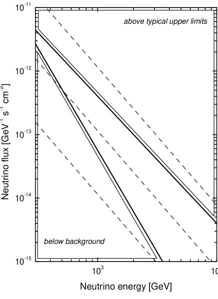
Figure 1: Fluxes of neutrinos produced in the framework of different models of hadronic microquasars as compared with the atmospheric neutrino background and the upper limits for typical sources obtained by AMANDA-II.

Table 1: Comparison between upper limits and predictions of the photopion model for some microquasars.

Microquasar	Prediction	Upper limit
	(Distefano et al. 2002)	(data from Ahrens et al. 2003)
	erg cm-2 s-1	erg cm-2 s-1
SS433	1.7E-9	2.6E-10
Cyg X-3	4.0E-9	1.3E-9
Ci Cam	2.2E-10	2.9E-10

4 Concluding remarks

It is clear that, with the appearance of km-scale detectors, neutrino astronomy will soon become an interesting aid in the study of microquasars and other stellar objects. Here we have focused on showing that the current state of the art in neutrino observations can also be used to establish useful constraints on some of the hadronic models presented in the literature.

Acknowledgements

We thank D. Purmohammad for insightful comments regarding the proton flux treatment. D.F.T. research is done under the auspices of the US Department of Energy (NNSA), by the UC’s LLNL under contract W-7405-Eng-48. G.E.R. is supported by Fundación Antorchas, ANPCyT (PICT 03-04881), and CONICET (PIP 0438/98). This research benefited from the ECOS French-Argentinian cooperation agreement.

References

- [1] Ahrens J., et al. 2004, Phys. Rev. Lett. 92, 071102
- [2] Bednarek W., Giovannelli F., Karakula S., et al. 1990, A&A, 236, 268
- [3] Dar, A., & Laor, A. 1997, ApJ, 478, L5
- [4] Dermer C. D. 1986, A&A, 157, 223
- [5] Distefano, C., Guetta, D., Waxman, E., & Levinson, A. 2002, ApJ, 575, 378
- [6] Drury, L.O’C., Aharonian, F.A., Völk, H.J. 1994, A&A, 287, 959
- [7] Falcke, H. & Biermann, P. L. 1995, A&A, 293, 665
- [8] Ghisellini, G., Maraschi, L., & Treves, A. 1985, A&A, 146, 204
- [9] Hayakawa S. 1969, “Cosmic ray physics: nuclear and astrophysical aspects”, New York, Wiley-Interscience
- [10] Lamers, H. J. G. L. M. & Cassinelli, J. P. 1999, Introduction to Stellar Winds, Cambridge University Press, Cambridge
- [11] Levinson, A., & Waxman E. 2001, Phys. Rev. Lett., 87, 171101
- [12] Migliari, S., Fender, R. & Méndez, M. 2002, Science, 297, 1673
- [13] Purmohammad, D. & Samimi, J. 2001, A&A 371, 61
- [14] Romero G. E. & Torres D. F. 2003, ApJ 586, L33
- [15] Romero, G. E., Torres, D. F., Kaufman-Bernadó, M. M. & Mirabel, I. F. 2003, A&A, 410, L1
- [16] Torres D. F., Domingo-Santamaría E., & Romero G. E. 2004, ApJ 601, L75