The IC 133 Water Vapor Maser in the Galaxy M33:
A Geometric Distance

Abstract

We report on the results of a 14 year long VLBI study of proper motions in the IC 133 H₂O maser source in the galaxy M33. The method of Ordered Motion Parallax was used to model the 3-dimensional structure and dynamics of IC 133 and obtain a distance estimate, 800 $\pm$ 180 kpc. Our technique for determining the distance to M33 is independent of calibrations common to other distance indicators, such as Cepheid Period-Luminosity relations, and therefore provides an important check for previous distance determinations.

1 Introduction

Calibration of the extragalactic distance scale (EDS) is of crucial importance to modern (precision) cosmology. Robust estimates of the local expansion rate of the universe, H_∘, bear on calculation of cosmological parameters such as flatness, the Cosmological constant, and the equation of state of dark energy (e.g., Freedman et al., 2001; Spergel et al., 2003). However, estimation of the EDS involves layers of calibration and a variety of techniques, objects, and effects, which makes assessment of systematic error difficult.

The best estimate of H_∘ to date has been provided by the Hubble Space Telescope (HST) Key Project (hereafter referred to as the Key Project; Freedman et al., 2001). Key Project researchers first calibrated Period-Luminosity (PL) relations for Cepheid variable stars in the Large Magellanic Cloud (LMC) and applied them to hundreds of variables observed with the HST in 31 relatively nearby ($<$ 30 Mpc) galaxies. They then used the resulting distance estimates to bootstrap calibration of other distance indicators (e.g., Tully-Fisher) in the range 60$-$400 Mpc. H_∘ was estimated from the entire sample of galaxies.

Conceptually, the weakest link in determination of the EDS is that it depends on the distance to a single galaxy, the LMC, which remains controversial. So-called short and long distances have been obtained from analyses of a variety of datasets for distance indicators such as detached eclipsing binaries and red clump stars. The uncertainty in the distance to the LMC may be as small as 5% (Key Project), but the spread in distance estimates is larger than the formal errors, which suggests an uncertainty a few times larger than this (e.g., Feast & Catchpole, 1997; Fitzpatrick et al., 2003; Guinan et al., 1998; Kanbur et al., 2003; Stanek et al., 2000; Udalski, 2000). Other problems arise from the poorly understood structure of the LMC (van der Marel, 2004, and references therein) and uncertainty in the effect of metalicity on PL relations (Groenewegen et al., 2004, and references therein), the latter being important in as much as the LMC is relatively metal poor compared to galaxies targeted by the Key Project.

Prior to the work reported here, NGC 4258 was the only galaxy for which a distance had been estimated from the analysis of H₂O maser source structure and dynamics. For NGC 4258, proper motions and accelerations of maser components were measured and fit to a model of a thin disk with circular orbits in Keplerian rotation. A distance estimate of 7.3 $\pm$ 0.3 $\pm$ 0.4 Mpc was obtained (Herrnstein et al., 1999). The two errors are statistical and systematic, respectively, with the latter being due in large part to a relatively weak constraint on orbital eccentricity. The maser distance estimate is very important, since it provides a check of the supporting calibrations in Cepheid and other non-maser distance estimates. The NGC 4258 maser distance was found to agree reasonably well with the Key Project distance (7.8 $\pm$ 0.3 $\pm$ 0.5 Mpc), after adoption of PL relations derived from Optical Gravitational Lensing Experiment (OGLE) data (Newman et al., 2001; Freedman et al., 2001). However, the Cepheid data for NGC 4258 is rather poor (e.g., only 15 comparatively metal rich stars with a limited range of periods), and it remains possible that some terms in the Key Project error budget are larger than originally believed.

Cepheid and maser distances to NGC 4258 and other nearby galaxies would permit robust quantification of the EDS. Detectable H₂O maser emission within Local Group galaxies is comparatively rare; it is known in M33, IC 10, and the Magellanic Clouds. Because it is relatively nearby, M33 is an important target for such study. The IC 133 maser in a star forming region of M33 is only of moderate strength ($\sim$ 1$-$2 Jy), but it exhibits numerous Doppler components spread over $\approx$ 50 km s^-1, which is important for the construction of accurate dynamical models.

M33 has been the target of many previous non-maser distance studies. Table 1 gives a representative sampling of recent distance estimates to this Local Group galaxy. Many of the quoted errors appear to be small, $\approx$ 5%, but none of the techniques employed were independent of the assumptions and calibrations that plague all primary and secondary distance indicators. In this paper we report on the results of a VLBI study of H₂O masers in IC 133. As with the NGC 4258 maser distance, the method employed here is independent of the calibrations implicit in previous optical distance determinations.

Spectral line VLBI observations of H₂O maser proper motions have been used successfully to find distances to a number of high mass star-forming regions in our own Galaxy. These include the Orion Kleinmann-Low (KL) nebula (Genzel et al., 1981a), W51 Main (Genzel et al., 1981b), W51 North (Schneps et al., 1981), Sgr B2 North (Reid et al., 1988), and W49 N (Gwinn et al., 1992). In some of the Galactic star-forming regions maser motions appeared random, so a simple statistical comparison of the spread in radial velocities to the spread in transverse velocities (derived from proper motions) was made to obtain a distance. In other sources maser motions appeared ordered and a dynamical model was fit to the observed proper motions and radial velocity distribution, giving distance as a parameter of the fit. The techniques are called Statistical Parallax and Ordered Motion Parallax, respectively.

Because IC 133 is much weaker (due to its far greater distance) than any Galactic H₂O maser source, its observation requires a much longer time baseline. At the distance of IC 133 a typical transverse velocity of 30 km s^-1 corresponds to a proper motion of $\approx$ 10 $\mu$as yr^-1. Since the motions of the weaker maser spots are expected to have errors of this magnitude, many years are required for a successful observation. We, therefore, undertook a 14 year long VLBI study to track proper motions and determine a distance using techniques that have been successfully applied to Galactic H₂O maser sources. In $\S$2 we present the details of the VLBI observations, calibrations, and results; in $\S$3 we present separate millimeter wave observations of the IC 133 maser region that provide independent parameter constraints for our modeling; in $\S$4 we outline the proper motion modeling and present results; and in $\S$5 we draw conclusions about the importance of our geometrical technique for determining extragalactic distances.

2 22 GHz VLBI Investigations

2.1 Observations

Observations of the H₂O maser in IC 133 were made using the US VLBI network and its successor the VLBA, operated by the National Radio Astronomy Observatory (NRAO) The maser was observed on eight different occasions between 1987 and 2001 (Table 2). Approximately 9 hours was spent on-source during Epoch 1, 14 hours during each of Epochs 2$-$7, and 1.5 hours during Epoch 8. In order to minimize systematic errors, we kept the arrangement of proper motion measurements, the array, the sequence of scans, the source lists, and the LO tuning as fixed as possible from epoch to epoch. Two epochs, Epoch 8 and the second day of Epoch 1, i.e., June 7, required slightly different observational setups, since a second maser, M33.19 (Huchtmeier et al., 1978; Israel & van der Kruit, 1974), was also observed. In particular, during Epoch 8 and the second half of Epoch 1, we switched rapidly between IC 133, one or more calibrators, and M33.19, while in Epochs 2$-$7 we observed 1.75 hour blocks of IC 133, bracketed by calibrators. Rapidly switched observations were made so that the relative angular motions of IC 133 and M33.19 could be measured and an independent distance to M33 obtained. The results of the rapid switching observations of Epoch 8 will be reported by Brunthaler, Reid, & Falcke (in preparation). The data were correlated at the Mark III Haystack correlator (epochs 1$-$5) and at the VLBA correlator (Epochs 6$-$8).

The Mark III video converters (VCs) or VLBA Baseband converters (BBCs) were set so that the full range of emission from IC 133, as observed in 1987 April, could be covered (Greenhill et al., 1990). In most cases, we used three slightly overlapping 2 MHz ($\approx$ 27 km s^-1) bands set at center frequencies corresponding to the velocities $-$216.28, $-$240.35, and $-$264.43 km s^-1, with respect to the local standard of rest (LSR). (See Table 3 for details.) In the first two epochs, three of the other VCs were set redundantly to protect against recording faults and in Epochs 3$-$7 four of the VCs or BBCs were set in a manner so that a multi-band delay analysis could be performed (see $\S$2.2.1$-$2 below). In Epoch 8, a single 8 MHz wide band was employed for IC 133 observations. We observed left circular polarization throughout.

2.2 Calibration

We employed different calibration schemes for epochs 1$-$5 than we did for epochs 6$-$8 because we 1) used different arrays for the two groups of epochs and 2) took advantage of more sophisticated implementations of various processing tools for the latter group of epochs.

2.2.1 Epochs 1$-$5

After correlation, the data from Epochs 1$-$5 were translated to the NRAO Mark II data format and processed with the spectral-line VLBI software package at the Center for Astrophysics (CfA) in Cambridge, MA. Post-correlation data reduction included amplitude, delay, and phase calibrations. Amplitude calibration involved correcting cross power spectra for bandpass response and variations in station gain and atmospheric opacity. Delay calibration refined station clocks and drift rates and was based on observations of a few strong quasars, including 3C 345, 3C 454.3, 0234$+$285, and NRAO150. Phase calibration corrected for variations induced by atmospheric and frequency standard fluctuations and was based on a technique called spectral “phase referencing”, whereby the phase of one spectral channel (the “reference feature”) was subtracted from the phases of all other spectral channels. See Reid et al. (1980) for details. A small part of the processing was accomplished in a non-standard fashion with Haystack Observatory spectral-line software and is described below.

In an effort to reduce delay errors and hence relative position errors of maser “spots” in synthesis maps, we employed a non-standard method of delay calibration for Epochs 3$-$5. Having set the non-maser VCs in these epochs to appropriate values, a multi-band analysis was performed by first running the Haystack FRNGE program (in manual phase cal as opposed to extracted phase cal mode) on all calibrator scans to determine multi-band delay residuals. These residuals were then used to correct Haystack a priori single-band clocks, which had different values since they referred to different points in the signal path. After correcting the Haystack a priori clocks, we solved for a single linear drift rate for each station and a possible clock jump between the “two days” of each epoch. (Each of the three epochs consisted of 17 hours of observations, a 7 hour break, and another 17 hours of observations.) The clock drift rates obtained were then applied to CfA single-band data to determine actual clocks.

Clock drift rate errors averaged 0.7, 4.3, and 3.2 ns day^-1, while clock errors averaged 0.4, 2.4, and 1.8 ns, for Epochs 3, 4, and 5, respectively. We attribute the higher errors in Epoch 4 to poor weather at NRAO and the fact that Haystack did not observe and in Epoch 5 to poor weather at both NRAO and Haystack. In contrast, Epoch 2 drift rate and clock errors were $<$ 8.6 ns day^-1 and $<$4 ns, respectively and Epoch 1 clock errors were as high as 22 ns.

2.2.2 Epochs 6$-$7

After correlation, the data from Epochs 6$-$7 were imported directly into NRAO’s Astronomical Image Processing System (AIPS) software package. Amplitude, multi-band delay, and phase calibrations were carried out in the standard fashion for spectral line VLBI data. Spectral “phase referencing” was accomplished by extracting a “reference feature” from the main band (the $-$216.28 km s^-1 band), self calibrating to remove residual phase and amplitude errors, and applying the solutions to the entire data set.

2.2.3 Epoch 8

Epoch 8 data were reduced in the standard fashion until the “phase referencing” step. In this epoch absolute phases were determined, in contrast to the relative phases (relative to a given feature, called the “reference feature”) that were determined for the seven previous epochs. The quasar, J0137$+$312, was used to accomplish this. Further details will be reported in a future paper (Brunthaler et al., in preparation).

2.3 Imaging

In agreement with Greenhill et al. (1990, 1993), we have identified three centers of maser emission: 1) an area near the reference feature, which was typically located at an LSR velocity of about $-$210 km s^-1, 2) an area 25 mas east and 15 mas south of the reference feature, and 3) an area 290 mas west and 45 mas south of the reference feature. In Greenhill et al. (1990), regions 1), 2), and 3) were called IC 133 Main, IC 133 Southeast, and IC 133 West, respectively. We now refer to 1) and 2) together as IC 133 Main (since the two regions are separated by $\sim$ 0.1 pc and are probably associated with the same star-forming region) and 3) as IC 133 West.

Having detected no new areas of emission in any of the epochs, we made three small, high resolution maps in each band. In particular, we imaged (with natural weighting) and CLEANed each spectral channel map in $256\times 256$ pixel boxes centered on: (0.000,0.000), (0.024,$-$0.015), and ($-$0.288,$-$0.044) mas. Because the restoring beams varied by up to a factor of two in each direction among the epochs (Table 2), the pixel sizes and hence box sizes varied too. The average box size was $16.4\times 16.4$ mas. Epochs 1$-$5 were imaged and CLEANed with the NRAO AIPS task MX and Epochs 6$-$8 were imaged and CLEANed with the AIPS task IMAGR. The (u,v)-data were variance weighted to maximize the sensitivity of maps.

After imaging, selected peaks were fit with a two dimensional Gaussian to determine their flux density and x and y offsets from the reference feature. Most spurious maser spots were rejected by requiring that the following three constraints be met:

1) Peaks have a flux density of at least 5 times the channel rms (Table 2).

2) Peaks have a flux density of at least 1.3 times the absolute value of the largest negative peak in the channel map.

3) Peaks persist over two or more adjacent channels at approximately the same position ($<$ beam).

The last constraint was relaxed slightly when groupings of related peaks, called “features”, were found to persist over many epochs. In particular, when features persisted over three or more epochs, we accepted single channels that met the other two constraints.

Maps from individual epochs were then referred to a common origin by selecting a strong and relatively isolated feature that was present during all eight epochs (Fig. 1). The accuracy of the registration varies from epoch to epoch and depends on factors such as the reference feature’s peak intensity, the number of channels that compose the feature, and the presence or absence of significant systematic error during the epoch. See $\S$2.4.1 for details of the error model.

2.4 Results

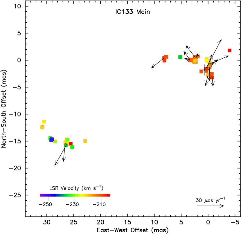
Figure 2: Map of features and proper motions in IC 133 Main. A constant vector has been subtracted from all proper motions such that their weighted mean is zero. Radial velocities are indicated by color. Note that features cluster along two arcs, one on either side of an ellipse with position angle $-65^{\circ}$. Redshifted features tend to lie near the origin, while blueshifted features tend to lie to the southeast. Note that the absence of arrows for many features does not imply that there is no motion in the underlying gas. The cross near the origin marks the location of the center of expansion.

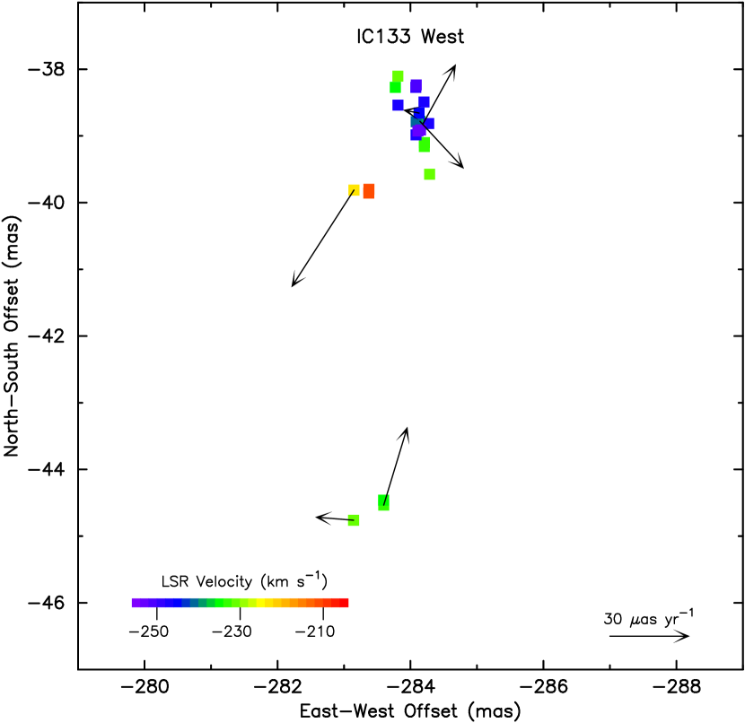
Figure 3: Map of features and proper motions in IC 133 West. See the Fig. 2 caption for details.

The maser features in IC 133 Main (Fig. 2) appear to trace out two short arcs, one on each edge of an ellipse with major axis $\sim$ 30 mas, minor axis $\sim$ 10 mas, and position angle $\sim$ $-$65^∘, measured east of north. The redshifted spots tend to be clustered on one side of the ellipse and the blueshifted spots on the other side. Most of the proper motions are directed outwards from the center of the ellipse. In IC 133 West (Fig. 3), features are clustered in two regions: the more densely populated region is centered at an offset of $\sim$ ($-$284,$-$39) mas and the less densely populated region, consisting of just three spots, is centered at an offset of $\sim$ ($-$283.5, $-$45) mas. The proper motions in IC 133 West are few and appear to be random.

Table 4 shows the peak flux denisty, right ascension and declination offsets, and uncertainties for all 81 features in IC 133 Main and 25 features in IC 133 West. Proper motions were determined for 16 of the features in IC 133 Main and 6 of the features in IC 133 West. Four additional features, even though they persisted over three or more epochs (as did the 22 features for which proper motions were determined), were deemed too spectrally blended for an accurate proper motion determination.

2.4.1 Position Errors

The formal uncertainty in fitted position for unblended maser spots is given by $\Delta\theta_{fit}\sim 0.5\theta_{b}\Delta S/S$, where $\theta_{b}$, $\Delta S$, and $S$ are the synthesized beam size, image rms, and peak intensity, respectively (Reid et al., 1988). Since the position angles of the restoring beams are all close to zero (Table 2), we substituted the restoring beam major and minor axes to obtain uncertainties in right ascension and declination, respectively. As an example, the peak channel of the reference feature in Epoch 7 has formal uncertainties of 0.7 $\mu$as and 2.5 $\mu$as in right ascension and declination offsets, respectively. Since the reference feature is an average of a number of channels, however, its formal uncertainty is somewhat smaller.

The uncertainty in the absolute position of the reference feature gives rise to one of the largest sources of known systematic error in synthesis maps. The position error of a maser spot in synthesis maps, $\Delta\theta_{spot}$, is related to the position error of the reference feature, $\Delta\theta_{ref}$, by $\Delta\theta_{spot}=(\Delta\nu/\nu)\Delta\theta_{ref}$, where $\nu$ is the frequency of the maser spot and $\Delta\nu$ its frequency offset from the reference feature (Thompson, Moran, & Swenson, 2001). Since the reference feature is known to an accuracy of $\sim 0{\hbox to0.0pt{.\hss}}^{{}^{\prime\prime}}\!1$ in each coordinate, maser spots offset by 1 MHz (13.5 km s^-1) from the reference feature will be subject to systematic position offset errors of $\sim$ 5 $\mu$as. For most epochs, systematic errors arising from the reference feature’s absolute positional uncertainty are roughly the same for a given feature and hence do not strongly affect proper motions. This is because the reference features in those epochs lie within $\sim$ 2 km s^-1 of one another (all close to $-$210 km s^-1). In two epochs, however, blending near $-$210 km s^-1 forced us to choose reference features at $-$216.28 km s^-1 (Epoch 3) and $-$220.49 km s^-1 (Epoch 7). The total spread in reference feature LSR velocities is 12.4 km s^-1, which could lead to errors that differ by as much as 4 $\mu$as from one epoch to another for a given feature.

Clock offset errors are another source of systematic error. In Epoch 1 delay errors were found to be 22 ns on VLA baselines and 7 ns on non-VLA baselines. Since VLA baselines are among the most sensitive baselines in the experiment, systematic errors in synthesis maps will be quite significant for this epoch. Greenhill et al. (1993) did a Monte Carlo simulation to assess the impact of delay and other systematic errors on synthesis maps in Epochs 1 and 2 as a function of frequency or LSR velocity. They found $\sim$0.13 and 0.57 $\mu$as (km s^-1)^-1 for right ascension and declination errors, respectively (Epoch 2) and $\sim$0.59 and 2.5 $\mu$as (km s^-1)^-1 for right ascension and declination errors, respectively (Epoch 1). These refer to errors within the reference band. In Epochs 3$-$7, we employed a multi-band analysis to correct clock offsets and drift rates and do not believe residual errors in these quantities to be significant.

When maser spots are weak the root-sum-square of the individual errors described above is a good estimate of the total error. This is because weak spots are signal-to-noise limited and the effects of unknown systematic errors do not significantly change the error estimate. When spots are strong, however, the root-sum-square above is almost certainly an underestimate of the real error. Strong spots are dynamic range limited, not signal-to-noise limited, which means that unknown systematic errors play a much larger role. Because of this unknown and unaccounted for error, we assign a minimum position error of 10 $\mu$as in each coordinate. Note that this refers to individual channels and not to features, which are typically composed of many channels.

2.4.2 Proper Motions

There are two ways to determine proper motions:

1) The feature method where related channels in a given epoch are grouped into features and proper motions are found from the best fit to feature positions as a function of time.

2) The channel method where individual channels are analyzed for motion and a weighted average of all motions among related channels is calculated.

Since many of our features appear to be spectrally blended, possibly due to the amplification of different hyperfine components (see $\S$2.4.3 below), we prefer the “channel method” to determine proper motions.

Table 5 shows the results of the “channel method” in both IC 133 Main and IC 133 West. We note that our channel-by-channel analysis was complicated by the fact that the eight epochs had three different spectral resolutions or channel widths: epochs 1$-$5 had a resolution of 0.4808 km s^-1, epochs 6$-$7 had a resolution of 0.2106 km s^-1, and epoch 8 had a resolution of 0.843 km s^-1. In order to get channel motions, we assumed that channels were separated by 0.4808 km s^-1 (because an epoch 1$-$5 data point was present for all motions) and if a feature persisted into epochs 6$-$8, we paired up all smaller (or larger) resolution channels that fell within $\pm$0.24 km s^-1 of the 0.4808 km s^-1 channel. This meant, for example, that a single epoch 1$-$5 channel could be paired up with two (and sometimes three) epoch 6$-$7 channels. We fit all pairings but because they were not all independent we adjusted the weighted averages and error estimates accordingly. For example, the right ascension proper motion error for Feature 4 in IC 133 West is given by $[0.5/(5.91)^{2}+0.5/(5.86)^{2}+1/(6.40)^{2}]^{-1/2}$, since the first and second channel motions are not independent.

Table 6 shows a comparison between the “channel” and “feature” methods of determining proper motions in IC 133 Main. In the “channel method”, we required that two criteria be met for a motion to be retained: 1) a channel had to persist over at least three epochs and 2) there had to be at least two such channels to average. In the “feature method”, we asked that individual position errors (i.e., for a feature in a particular epoch) not deviate by more than 3-$\sigma$ from the least squares fit to all the epochs. This was accomplished by either using the error model as is or by doubling all errors in the error model. Seven of the sixteen motions determined by the “feature method” required a doubling of all position errors and one feature could not be fit even then. Thus, even though the two methods give compatible results, the “channel method” appears to be better suited to spectral blends, since it does not require that we artificially inflate errors in order to obtain motions.

2.4.3 Spectra

We constructed IC 133 spectra, total imaged flux density (Jy) as a function of LSR velocity, from the fitted peaks in synthesis maps (Fig. 4). When a channel had no peaks that fit the three criteria above, the flux density was set to the 5-$\sigma$ noise level for that epoch. In the first epoch we plotted results from the main band (the $-$216.2 km s^-1 band) only, since there were no fitted peaks in the remote bands. In the other epochs we do not display the $-$264.43 band because there were only two believable (and weak) fitted maser spots in this band.

Figure 5 shows the time evolution of a spectrally blended feature in IC 133 Main. There are at least two explanations for such blending. First, it could be due to the simple superposition of features. Second, it could be due to amplification of different hyperfine components at different times. The $6_{16}-5_{23}$ transition of H₂O is split into six hyperfine components that span $\sim$ 6 km s^-1 in LSR velocity (Walker, 1984). Under the extreme non-LTE conditions of a typical H₂O maser region, the relative intensities of the hyperfine components might be expected to vary a great deal over time and bear little resemblance to LTE ratios. Walker (1984) did a statistical study of 386 H₂O maser features in W49N and found that all six hyperfine components were present, not just the three strongest ones. The complicated spectral blend located near ($-$0.2,$-$1.0) mas (Fig. 5) spans $\sim$ 6 km s^-1 in LSR velocity and varies quite a bit from epoch to epoch. This variation might be caused by different hyperfine components being more strongly amplified in different epochs.

3 Owens Valley MM Array Investigations

We observed four transitions, CO J=1$\rightarrow$0, CO J=2$\rightarrow$1, HCN J=1$\rightarrow$0 and HCO$+$ J=1$\rightarrow$0 with the Owens Valley Radio Observatory’s Millimeter Array between 1998 April and 1999 February (Table 7). The CO J=1$\rightarrow$0 observing band consisted of 128 spectral channels at a velocity resolution of 0.65 km s^-1, the CO J=2$\rightarrow$1 observing band consisted of 64 spectral channels at a velocity resolution of 0.65 km s^-1, and the HCN J=1$\rightarrow$0 and HCO$+$ J=1$\rightarrow$0 observing bands consisted of 32 spectral channels at velocity resolutions of 0.85 and 0.84 km s^-1, respectively. The CO J=1$\rightarrow$0 band was centered at $-$230 km s^-1 and the others were centered at $-$222 km s^-1.

Calibration consisted of the following: a flux calibration (using a primary calibrator such as Neptune), a passband calibration (using observations of a strong quasar such as 2145$+$067), and a gain calibration. After calibration, we combined the (u,v)-data sets from the seven CO J=1$\rightarrow$0 tracks (low, high, and ultrahigh resolution configurations) and mapped and CLEANed all 128 channels with the AIPS task IMAGR using a restoring beam of $2{\hbox to0.0pt{.\hss}}^{{}^{\prime\prime}}\!2\times 1{\hbox to0.0pt{.\hss}}^{{}^{\prime\prime}}\!8$. Similarly, we combined the (u,v)-data from the two CO J=2$\rightarrow$1 tracks and mapped and CLEANed all 64 channels using a restoring beam of $1{\hbox to0.0pt{.\hss}}^{{}^{\prime\prime}}\!0\times 0{\hbox to0.0pt{.\hss}}^{{}^{\prime\prime}}\!8$. After mapping, we found the moments in the two images using the AIPS task XMOM. Figure 6 shows the zeroeth moment of the two transitions, superimposed on the same map, and Fig. 7 shows spectra, constructed by plotting the total imaged flux density within a small area as a function of LSR velocity.

4 Discussion

There are two techniques to estimate distances from H₂O proper motion measurements. The first, Ordered Motion Parallax, is appropriate for sources that can be described by simple models where distance is a parameter, e.g., spherically symmetric outflow or symmetrical rotation. In this technique, a dynamical model is fit to observed proper motion and LSR velocity distributions. The distance is one of the parameters of the fit that is necessary to couple proper angular motions and linear line of sight velocities. This technique has been used successfully to estimate the distance to a number of Galactic star-forming regions including Sgr B2N (Reid et al., 1988). A second and simpler technique, Statistical Parallax, is appropriate for sources with isotropic random motions (Trumpler & Weaver, 1953). The distance is given by $D$ = $\sigma_{R}/\sigma_{T}$, where $\sigma_{R}$ and $\sigma_{T}$ are the dispersions in radial Doppler motions and in transverse angular motions, respectively. This method has also been used successfully to find the distance to a number of Galactic star-forming regions including W51 M (Genzel et al., 1981b), W51 N (Schneps et al., 1981), and Orion-KL (Genzel et al., 1981a). We also used it in a preliminary distance estimate to M33 (Greenhill et al., 1993).

4.1 IC 133 Main

4.1.1 The Model

The structure and velocities of IC 133 Main (Fig. 2) suggest that it can be modelled as uniform outflow from a central source. For each maser feature we have measured a radial velocity, $v_{z}$, and the position offsets, $x$ and $y$. In addition, we measured two components of proper motion, $v_{x}$ and $v_{y}$, for all maser features that persisted over three or more epochs. Seven global parameters are unknown: distance to the source, $D$; the velocity of expansion, $V_{exp}$; the velocity in the plane of the sky of the center of expansion with respect to the reference feature, $v_{x_{0}}$ and $v_{y_{0}}$; the radial velocity of the center of expansion, $v_{z_{0}}$; and the sky position of the center of expansion, $x_{0}$ and $y_{0}$. In addition, the positions of the masers along the line of sight, $z$, are unknown. These parameters are related by the equations (Reid et al., 1988):

$$v_{x}={V_{exp}\over d}{(x-x_{0})\over R}+v_{x_{0}},$$

$$v_{y}={V_{exp}\over d}{(y-y_{0})\over R}+v_{y_{0}},$$

$$v_{z}=V_{exp}{z\over R}+v_{z_{0}},$$

where $R=[(x-x_{0})^{2}+(y-y_{0})^{2}+z^{2}]^{1/2}$ and $d=D/D_{0}$, with $D_{0}$ being an a priori distance.

Initial estimates of the global parameters and the radial offsets provide a starting point to the fitting procedure. We assume that:

1) $D_{0}$ is 700 kpc. This number is used solely to convert the units of observed proper motion from $\mu$as yr^-1 to km s^-1. Our choice does not affect the outcome.

2) $V_{exp}$ and $v_{z_{0}}$ are constrained as outlined below.

3) $v_{x_{0}}$ and $v_{y_{0}}$ are the weighted averages of $v_{x}$ and $v_{y}$, respectively.

4) ($x_{0},y_{0}$) is (0,0).

5) the radial offsets, $z$, are estimated from Eq. (3) and 2) above.

One additional point deserves special mention. Our experience with other H₂O masers such as Sgr B2N (Reid et al., 1988), as well as residuals to initial fits of the IC 133 velocity field, lead us to expect significant turbulent motions intrinsic to the source. In Sgr B2N, these motions are $\sim$ 15 km s^-1. We adopt this value for IC 133, which is reasonable given a resulting reduced $\chi^{2}\sim$ 1 for fits. Following Reid et al. (1988), we assigned weights to the velocity data by combining this turbulent velocity in quadrature with the measurement uncertainties.

4.1.2 Observations Used to Constrain the Solution

Because of substantial correlations between the expansion velocity ($V_{exp}$), the systemic velocity ($v_{z_{0}}$), and the distance (D), we seek independent estimates for $V_{exp}$ and $v_{z_{0}}$ in IC 133 Main.

The range of likely expansion velocities in IC 133 Main can be estimated by comparison with the most powerful Galactic H₂O masers. IC 133 Main resembles these sources in a number of ways. First, it is comparable in scaled flux density to the four most luminous H₂O maser sources in our Galaxy. Scaled flux density is the flux density that would be observed if all sources were moved to the distance of IC 133. Table 8 shows the peak flux densities of the four most luminous Galactic H₂O masers, scaled to a distance of 850 kpc, an unweighted average of the 13 M33 distance estimates in Table 1.

Second, the radial velocity span in IC 133 Main is similar to what one would expect to see in the strongest Galactic masers, were they moved to the distance of M33. For example, the range in detectable features for W49 N at 850 kpc is only $\sim$ 14 km s^-1 (Walker, Matsakis, & Garcia-Barreto, 1982). It is therefore likely that IC 133 has many weak high velocity features spanning decades or more in radial velocity that are simply below our detection limit.

Third, IC 133 resembles the most powerful Galactic H₂O masers both spatially and spectrally. Fig. 6 of Greenhill et al. (1990) shows a spot map of W49 N, were it at the distance of M33. The spatial extent and distribution of W49 N at this distance is very similar to the spatial extent and distribution of maser spots in IC 133 Main. Spectrally, IC 133 is skewed, with most of its strong features to one side of its peak. Three of the four Galactic masers in Table 8 (including W49 N) have simliarly skewed spectral distributions.

Not only does the H₂O maser in IC 133 Main resemble the most powerful Galactic H₂O masers, but the compact continuum emission associated with it does as well. In particular, (Greenhill et al., 1990) fit their 15 GHz IC 133 continuum data to a model of an optically thin homogeneous spherical H II region. For an observed flux density of 5.5 $\pm$ 0.5 mJy, they calculated the number of Lyman continuum photons in the H II region to be 2.8 $\times$ 10⁵⁰ s^-1. This, they point out, is consistent with the presence of several O4 stars. (Genzel et al., 1978) present VLBI observations of 12 Galactic H₂O sources in regions of star formation. They suggest that each “center of H₂O activity” in a source be identified with a young, massive star. W49 N, for example, with the largest number of centers of H₂O maser activity (10), might then be associated with 10 OB stars.

The four most powerful Galactic H₂O masers have relatively high velocity flows, i.e., expansion speeds in the range 40-55 km s^-1. It is reasonable to assume that IC 133 does as well, and that its narrow range of observed radial velocities is simply a selection effect due to its great distance. Taking an average of the expansion speeds in Table 8 and an error equal to the standard deviation, we adopt an expansion velocity for IC 133 of 46$\pm$6 km s^-1.

The range of likely systemic velocities in IC 133 Main comes from independent CO observations. CO, which is an excellent tracer of compact regions of star formation including H₂O masers, consistently gives a systemic velocity of $-$222 km s^-1 for the giant molecular cloud associated with the IC 133 maser in M33 (Fig. 7). The systemic velocity error was taken to be the half width half maximum of the two spectra discussed in $\S$3. We note that even though the CO J=2$\rightarrow$1 emission is offset by $\sim 1^{\prime\prime}$ from the maser position, it is well within the contours of the CO J=1$\rightarrow$0 emission (Fig. 6). We suggest that the CO J=2$\rightarrow$1 image emphasizes a local “hot spot” in the giant molecular cloud that either 1) the much larger beam of the CO J=1$\rightarrow$0 observation ($2{\hbox to0.0pt{.\hss}}^{{}^{\prime\prime}}\!2\times 1{\hbox to0.0pt{.\hss}}^{{}^{\prime\prime}}\!8$) is unable to resolve or 2) is obscured owing to high optical depth in the CO J=1$\rightarrow$0 transition. Finally, internal motions within the cloud are expected to be small, meaning that the systemic velocity of the maser should not differ significantly from the measured CO velocities. A BIMA study of 148 giant molecular clouds in M33 (Engargiola et al., 2003), for example, shows that the average full width half maximum in velocity within a cloud is only 5 km s^-1. Thus we adopt the systemic velocity of the IC 133 Main H₂O masers to be $-$222 $\pm$ 5 km s^-1.

4.1.3 Fits to the Velocity Field

Initial fits to the IC 133 velocity data show that the center of expansion is not well determined. We have found two well defined local minima in the $\chi^{2}$-plane, one at (0.6,-1.8) mas and the other at (26.0,-13.4) mas, which lie near the northwest and southeast edges of the maser distribution, respectively. Reduced $\chi^{2}$ values for the two centers are $\approx$ 0.5 and 0.8, respectively. Fitted distances are comparable at the two centers and are $\approx$ 740 kpc. A third less robust local minimum lies near the center of the distribution and gives distances in the range 630$-$875 kpc. Reduced $\chi^{2}$ values for this region are $\approx$ 0.9. Since the northwest local minimum is stable and has the lowest reduced $\chi^{2}$, we did all subsequent fits at this position, but allowed for a 16% uncertainty in distance due to the uncertainty in the location of the center of expansion. We note that it is not unusual for H₂O maser sources to have centers of expansion that are not in the middle of the maser distributions. The four best-fitting models for the maser velocity field in W49 N (Gwinn et al., 1992) all give centers of expansion significantly offset from the center of the distribution. An even more asymmetric maser lies in Sgr B2N (Reid et al., 1988), whose center of expansion lies outside of the maser distribution. For the case of IC 133, we suggest a physical model in which the young star that drives the observed outflow is located near the front of a dense cloud core. The redshifted maser emission, which is tightly clustered in the sky, represents (constrained) flow into dense ambient material. The ralatively distant blueshifted emission represents flow that has “broken out” into lower density material.

Due to the substantial correlations between the expansion velocity, the systemic velocity, and the distance, we adopted the following analysis strategy. We solved for distances for a grid of fixed expansion and systemic velocities. We then fit a second order polynomial to distance as a function of systemic velocity for each value of expansion velocity in the grid (Fig. 8). The center grid value, $V_{exp}$ = 46 km s^-1 and $v_{z_{0}}$ = $-$222 km s^-1, gives us our distance estimate, and its fitting error, the random error due to “noise” in the proper motions. One component of systematic error arises from the 16% “center of expansion error” mentioned above. Further systematic errors come from the variation in distance of grid values corresponding to the error bars on $V_{exp}$ and $v_{z_{0}}$, also discussed above.

We find a distance to IC 133 (and M33) of

$$D(kpc)=800\pm 12\%\pm 16\%\pm 9\%\pm 4\%.$$

The quoted errors are due to random error, the systematic error arising from the uncertainty in the center of expansion, and the systematic errors due to lack of knowledge of $V_{exp}$ and $v_{z_{0}}$, respectively. Adding the four sources of error in quadrature, we obtain

$$D(kpc)=800\pm 22\%=800\pm 180,$$

Note that the method of Statistical Parallax can not be used to estimate the distance to IC 133 Main, due to the poor apparent distribution of masers. Even a constrained Statistical Parallax, i.e., a radial velocity distribution centered on an observed systemic velocity of $-$222 km s^-1, gives the unrealistically low distance of $\sim$ 200 kpc.

4.2 IC 133 West

The motions in IC 133 West appear to be random but are too few for a meaningful application of the method of Statistical Parallax.

5 Conclusions

We have mapped H₂O maser emission in IC 133 over 8 epochs, spanning 14 years. We detected 106 features and measured motions in two centers of activity, Main and West. The structure and dynamics of IC 133 Main suggest radial outflow from a central source; the motions in IC 133 West appear to be random. We have modelled the dynamics of IC 133 Main to estimate a distance to M33. In order to constrain parameters that are correlated, we independently estimated expansion speed from comparison to the strongest Galactic sources and systemic velocity from CO J=2$\rightarrow$1 and CO J=1$\rightarrow$0 observations. We obtained a distance of 800 $\pm$ 180 kpc.

Although our results with this data set do not give small enough errors for comparison with other distances to M33, the technique is potentially powerful. As mentioned above, a variant of Ordered Motion Parallax has been used to obtain a distance to the galaxy NGC 4258 with a 7% uncertainty. The “maser method” employed in this paper and for NGC 4258 is independent of the calibrations implicit in the distance indicators used in Table 1. The large scatter and small error bars in this table, even for very recent estimates, suggest that uncontrolled systematic errors still exist despite the application of much effort, which reinforces the need for independent, geometric techniques.

Figure 1: Spectra of the maser feature used to register maps for each epoch to a common origin.

Figure 4: Spectra of total imaged power in synthesis maps for each epoch. Measured peak flux densities were corrected by the multiplicative factor $\theta^{2}_{meas}/\theta^{2}_{beam}$, where $\theta^{2}_{meas}$ is the measured peak area and $\theta^{2}_{beam}$ is the beam area. No features were found in the second band (v${}_{LSR}<-230$ km s^-1) during Epoch 1 (1987 June) and only two weak features in the third band (v${}_{LSR}<-254$ km s^-1) for any epoch. We do not display the third band. For channels in which no maser emission was detected, the noise level is plotted (5-$\sigma$)

Figure 5: Time evolution of a spectrally blended feature in IC 133 Main. The blending could be due to either the superposition of features or the amplification of different hyperfine components. The filled squares in the 2001 March 27 panel indicate detection of flux in isolated channels.

Figure 6: Zeroeth moment of the CO J=1$\rightarrow$0 image (light contours) and the CO J=2$\rightarrow$1 image (heavy contours). The zeroeth moment is the flux density summed over all channels. The restoring beams were $2{\hbox to0.0pt{.\hss}}^{{}^{\prime\prime}}\!2\times 1{\hbox to0.0pt{.\hss}}^{{}^{\prime\prime}}\!8$ and $1{\hbox to0.0pt{.\hss}}^{{}^{\prime\prime}}\!0\times 0{\hbox to0.0pt{.\hss}}^{{}^{\prime\prime}}\!8$ for the CO J=1$\rightarrow$0 and CO J=2$\rightarrow$1 transitions, respectively. Contours are displayed at 10, 30, 50, 70, and 90% of the CO J=2$\rightarrow$1 maximum, $6.9587\times 10^{3}$ Jy beam${}^{-1}\times$ m s^-1. We assume a distance of 850 kpc in fixing the scale bar. The cross at the center marks the position of the maser.

Figure 7: Spectra for the CO J=1$\rightarrow$0 (upper) and CO J=2$\rightarrow$1 (lower) transitions. Spectra were constructed by plotting the total flux density within a small area as a function of channel. For CO J=1$\rightarrow$0 we summed flux density in a $5{\hbox to0.0pt{.\hss}}^{{}^{\prime\prime}}\!25\times 5{\hbox to0.0pt{.\hss}}^{{}^{\prime\prime}}\!45$ area centered on ($0{\hbox to0.0pt{.\hss}}^{{}^{\prime\prime}}\!525,0{\hbox to0.0pt{.\hss}}^{{}^{\prime\prime}}\!275$) and for CO J=2$\rightarrow$1 in a $1{\hbox to0.0pt{.\hss}}^{{}^{\prime\prime}}\!75\times 1{\hbox to0.0pt{.\hss}}^{{}^{\prime\prime}}\!5$ area centered on ($-0{\hbox to0.0pt{.\hss}}^{{}^{\prime\prime}}\!475,0{\hbox to0.0pt{.\hss}}^{{}^{\prime\prime}}\!55$). These areas correspond to the edges of the 10% contours of Figure 6.

Figure 8: Distance ($D$) as a function of systemic velocity ($v_{z_{0}}$) for each of five expansion velocities ($V_{exp}$) in IC 133 Main. Error bars indicate random fitting errors. The solid lines are weighted fits, assuming a second order polynomial.

Table 1: Previous Distance Estimates to M33

Study	Method Employed	Distance
		(kpc)
Kim et al. (2002)	TRGB	916$\pm$17
	RC	912$\pm$17
Lee et al. (2002)	Cepheids	802${}^{+73}_{-67}$
Freedman et al. (2001)	Cepheids	817${}^{+38}_{-37}$
Magrini et al. (2000)	Planetary Nebulae	840$\pm$90
Pierce, Jurcevic, & Crabtree (2000)	LPVs	933${}^{+58}_{-54}$
Sarajedini et al. (2000)	HB	929${}^{+71}_{-66}$
Lee, Freedman, & Madore (1993)	TRGB	871${}^{+41}_{-39}$
Freedman, Wilson, & Madore (1991)	Cepheids	847${}^{+36}_{-34}$
Christian & Schommer (1987)	Cepheids	692${}^{+49}_{-46}$
Mould (1987)	LPVs	890$\pm$135
Mould & Kristian (1986)	TRGB	912${}^{+135}_{-118}$
de Vaucouleurs (1978)	Cepheids	720$\pm$70

Table 2: VLBI Observations

Date	Epoch	Antennas	Notes	Major	Minor	P.A.	Noise Level
				(mas)	(mas)	(∘)	(mJy)
1987 June 5, 7	1	BKGYON	no data from N;	1.25	0.25	,173	60
			poor weather at K
1988 September 25$-$26	2	BKGYON		0.95	0.26	,166	25
1990 November 11$-$13	3	BKGYON	no data from N	0.75	0.16	$-$15	40
1991 May 29$-$30	4	BGY VLBA(1) N	poor weather at G	0.64	0.12	1$-$7	25
1991 November 9$-$11	5	BKGY VLBA(1) N	no data from N;	0.84	0.12	$-$13	35
			poor weather at K,G
1993 February 17$-$19	6	BY VLBA(9)	poor weather at	0.65	0.21	$-$11	35
			N. Liberty, Hancock
1993 September 21$-$23	7	BY VLBA(9)		0.85	0.24	$-$21	35
2001 March 27	8	VLBA		0.68	0.33	1$-$2	40

Table 3: Observed Bandpasses

Date	Epoch	Band center VLSR	Channel separation	Bandwidth
		(km s-1)	(km s-1)	(km s-1)
1987 June 5$-$7	1	$-$216.28, $-$240.25, $-$277.83	0.4808	$-$201 to $-$256, $-$262 to $-$293
1988 September 25$-$26	2	$-$216.28, $-$240.35, $-$264.43	0.4808	$-$201 to $-$280
1990 November 11$-$13	3	$-$216.28, $-$240.35, $-$264.43	0.4808	$-$201 to $-$280
1991 May 29$-$30	4	$-$216.28, $-$240.35, $-$264.43	0.4808	$-$201 to $-$280
1991 November 9$-$11	5	$-$216.28, $-$240.35, $-$264.43	0.4808	$-$201 to $-$280
1993 February 17$-$19	6	$-$216.28, $-$240.35, $-$264.43	0.2106	$-$203 to $-$278
1993 September 21$-$23	7	$-$216.28, $-$240.35, $-$264.43	0.2106	$-$203 to $-$278
2001 March 27	8	$-$233.93	0.8436	$-$180 to $-$288

Table 4: Maser Feature Positions

VLSR	Peak Fν	$\Delta x$	$\sigma_{x}$	$\Delta y$	$\sigma_{y}$	Epochs
(km s-1)	(Jy)	(mas)	(mas)	(mas)	(mas)	Observed
IC 133 Main:
$-$204.38	0.04	$-$3.984	0.017	1.799	0.053	6
$-$204.49	0.29	25.538	0.010	$-$15.480	0.049	5
$-$206.17	0.17	3.332	0.005	0.048	0.010	1234
$-$207.62	0.58	3.329	0.002	0.043	0.003	234567
$-$207.80	0.16	2.331	0.013	$-$0.171	0.027	8
$-$207.83	0.09	2.522	0.010	0.374	0.043	3
$-$207.86	0.05	2.437	0.011	0.488	0.041	2
$-$208.18	0.12	0.211	0.008	$-$1.559	0.019	678
$-$208.20	0.06	$-$0.730	0.011	$-$3.211	0.042	2
$-$208.22	0.05	3.309	0.026	0.033	0.054	8
$-$208.70	0.09	8.164	0.005	0.412	0.014	45678
$-$208.82	0.06	$-$0.300	0.006	$-$1.223	0.019	267
$-$208.82	0.25	2.384	0.004	0.518	0.013	12367
$-$208.86	0.06	$-$0.574	0.020	$-$3.057	0.070	7
$-$208.91	0.05	$-$0.590	0.017	$-$3.065	0.053	6
$-$209.30	0.13	0.462	0.004	$-$1.643	0.010	13456
$-$209.49	0.07	2.299	0.028	$-$0.288	0.139	1
$-$209.52	0.07	8.131	0.026	$-$0.080	0.127	1
$-$210.01	0.08	7.832	0.010	0.616	0.027	6
$-$210.01	0.10	7.769	0.010	0.622	0.032	7
$-$210.11	0.10	2.257	0.010	0.597	0.027	6
$-$210.20	0.27	1.259	0.019	$-$2.100	0.039	8
$-$210.22	0.16	3.091	0.010	$-$0.057	0.027	5
$-$210.51	0.15	3.030	0.010	0.008	0.027	6
$-$210.75	1.16	2.560	0.002	$-$0.257	0.002	12345678
$-$210.99	0.40	0.311	0.006	$-$1.982	0.009	345
$-$211.23	0.04	3.052	0.011	$-$0.059	0.074	5
$-$211.70	0.06	3.140	0.022	$-$0.016	0.108	1
$-$211.95	0.12	$-$0.699	0.003	$-$2.508	0.010	123678
$-$212.24	0.10	2.978	0.016	0.065	0.056	7
$-$212.32	0.07	2.357	0.033	0.487	0.068	8
$-$212.34	0.15	2.638	0.013	$-$0.262	0.060	3
$-$212.61	0.10	2.599	0.010	$-$0.234	0.027	4
$-$212.66	0.24	2.478	0.010	$-$0.236	0.013	7
$-$212.84	0.14	2.506	0.011	$-$0.272	0.035	6
$-$213.21	0.05	3.045	0.017	0.126	0.053	6
$-$213.39	0.12	1.923	0.005	0.710	0.014	3567
$-$213.40	0.46	$-$0.276	0.002	$-$1.285	0.003	12345678
$-$213.49	0.22	2.558	0.013	$-$0.178	0.047	7
$-$213.64	0.08	2.672	0.014	$-$0.107	0.042	6
$-$213.69	0.09	2.364	0.020	$-$0.087	0.070	7
$-$213.71	0.07	26.204	0.023	$-$15.572	0.071	6
$-$215.42	0.05	2.349	0.020	$-$0.198	0.070	7
$-$216.46	0.07	2.499	0.020	$-$0.364	0.073	2
$-$216.52	0.74	$-$0.330	0.002	$-$0.957	0.003	12345678
$-$217.24	0.05	2.528	0.017	$-$0.310	0.053	6
$-$217.73	0.33	26.235	0.003	$-$15.523	0.007	123456
$-$218.05	0.04	$-$0.250	0.023	$-$0.966	0.071	6
$-$218.44	0.04	22.846	0.011	$-$14.983	0.074	5
$-$218.45	0.11	0.002	0.004	$-$2.737	0.015	234567
$-$219.10	0.10	$-$0.203	0.013	$-$0.130	0.047	7
$-$219.65	0.09	$-$0.450	0.007	$-$0.631	0.026	1367
$-$219.78	0.13	2.522	0.012	$-$0.236	0.036	6
$-$219.81	0.04	30.804	0.015	$-$12.306	0.080	4
$-$219.89	0.22	26.548	0.005	$-$15.322	0.012	2346
$-$220.11	0.14	0.298	0.017	$-$0.064	0.053	6
$-$220.44	0.05	22.832	0.026	$-$14.985	0.054	8
$-$220.57	0.03	0.302	0.025	0.184	0.092	2
$-$220.58	0.04	26.229	0.023	$-$15.595	0.071	6
$-$220.61	0.20	26.271	0.013	$-$14.662	0.026	567
$-$220.86	0.04	30.850	0.033	$-$12.472	0.068	8
$-$221.34	0.06	2.431	0.026	$-$0.041	0.054	8
$-$222.45	0.06	30.499	0.022	$-$11.371	0.080	2
$-$222.79	0.02	26.192	0.023	$-$15.505	0.083	2
$-$222.81	0.03	26.487	0.022	$-$15.177	0.081	2
$-$224.86	0.04	0.222	0.025	$-$0.014	0.088	2
$-$229.24	0.04	28.440	0.022	$-$15.037	0.079	2
$-$230.20	0.08	25.326	0.016	$-$16.092	0.034	8
$-$231.03	0.09	26.150	0.015	$-$14.739	0.030	8
$-$234.61	0.11	5.170	0.010	0.613	0.032	7
$-$235.48	0.06	29.358	0.027	$-$14.427	0.093	7
$-$235.66	0.09	25.248	0.026	$-$16.107	0.054	8
$-$236.10	0.06	26.453	0.026	$-$15.771	0.054	8
$-$236.13	0.13	5.177	0.017	0.607	0.056	7
$-$236.98	0.05	5.196	0.019	0.541	0.054	6
$-$238.61	0.05	29.217	0.014	$-$14.775	0.054	4
$-$243.48	0.03	29.085	0.019	$-$14.649	0.061	2
$-$245.81	0.09	29.131	0.016	$-$14.743	0.055	4
$-$246.01	0.05	29.056	0.021	$-$14.642	0.071	7
$-$246.35	0.04	29.045	0.020	$-$14.685	0.054	6
$-$251.45	0.08	29.001	0.021	$-$14.678	0.054	6
IC 133 West:
$-$210.92	0.09	$-$283.375	0.015	$-$39.800	0.037	6
$-$211.13	0.19	$-$283.374	0.016	$-$39.856	0.048	7
$-$222.30	0.14	$-$283.149	0.010	$-$39.812	0.027	123
$-$230.97	0.17	$-$283.145	0.003	$-$44.761	0.008	2367
$-$230.97	0.16	$-$284.288	0.006	$-$39.573	0.011	245
$-$231.46	0.03	$-$283.810	0.018	$-$38.104	0.066	2
$-$231.69	0.11	$-$284.129	0.005	$-$38.694	0.013	3456
$-$232.21	0.06	$-$284.207	0.020	$-$39.158	0.070	7
$-$232.33	0.05	$-$284.209	0.023	$-$39.099	0.071	6
$-$233.37	0.10	$-$283.597	0.005	$-$44.535	0.013	24567
$-$234.35	0.03	$-$283.771	0.019	$-$38.272	0.070	2
$-$235.30	0.10	$-$284.184	0.007	$-$38.826	0.025	467
$-$235.81	0.03	$-$283.596	0.020	$-$44.461	0.073	2
$-$237.47	0.11	$-$284.142	0.003	$-$38.781	0.011	346
$-$241.37	0.07	$-$284.085	0.010	$-$38.786	0.043	3
$-$241.51	0.09	$-$284.114	0.011	$-$38.873	0.041	2
$-$244.44	0.20	$-$284.129	0.002	$-$38.657	0.005	234567
$-$246.86	0.06	$-$284.203	0.017	$-$38.491	0.053	6
$-$246.87	0.02	$-$283.811	0.022	$-$38.538	0.080	2
$-$247.15	0.03	$-$284.083	0.018	$-$38.983	0.065	2
$-$247.94	0.05	$-$284.274	0.016	$-$38.814	0.056	7
$-$249.89	0.09	$-$284.080	0.020	$-$38.271	0.070	7
$-$251.90	0.09	$-$284.087	0.014	$-$38.235	0.043	6
$-$252.01	0.07	$-$284.152	0.010	$-$38.911	0.027	4
$-$253.45	0.07	$-$284.112	0.029	$-$38.926	0.103	2

Table 5: Maser spot positions and proper motions

VLSR	Epochs	Position Offsets				Proper Motions
(km s-1)
		$\Delta x$	$\sigma_{x}$	$\Delta y$	$\sigma_{y}$	$\Delta v_{x}$	$\sigma_{v_{x}}$	$\Delta v_{y}$	$\sigma_{v_{y}}$
		(mas)				($\mu$as yr-1)
IC 133IC 133 Main:
Feature 1
$-$205.69	1234	3.339	0.008	0.030	0.021	$-$0.53	3.40	10.67	11.37
$-$206.17	1234	3.329	0.008	0.051	0.028	$-$2.61	3.17	14.55	11.51
$-$206.66	124	3.326	0.010	0.054	0.012	1.68	3.91	7.99	10.22
Weighted average		3.332	0.005	0.048	0.010	$-$0.78	1.99	10.82	6.34
Feature 2
$-$206.66, $-$206.60	35, 7	3.344	0.007	0.007	0.021	$-$32.04	8.96	56.28	29.22
$-$206.66, $-$206.81	35, 67	3.345	0.007	0.002	0.019	$-$25.32	6.08	40.51	18.19
$-$207.14, $-$207.02	2345, 67	3.341	0.005	0.045	0.011	10.83	3.25	$-$14.06	9.94
$-$207.14, $-$207.23	2345, 67	3.331	0.004	0.048	0.010	1.36	2.71	$-$7.67	8.36
$-$207.62, $-$207.44	2345, 67	3.323	0.004	0.050	0.006	$-$1.67	2.52	6.39	4.80
$-$207.62, $-$207.65	2345, 67	3.326	0.004	0.047	0.005	0.52	2.52	2.08	4.02
$-$207.62, $-$207.86	2345, 67	3.326	0.004	0.047	0.005	0.16	2.52	1.51	3.70
$-$208.10, $-$207.86	2345, 67	3.327	0.004	0.040	0.005	$-$1.59	2.52	4.50	3.84
$-$208.10, $-$208.07	2345, 67	3.325	0.004	0.040	0.005	$-$3.59	2.52	4.22	3.73
$-$208.10, $-$208.28	2345, 67	3.322	0.004	0.039	0.005	$-$5.83	2.52	3.85	3.66
$-$208.58, $-$208.49	45, 67	3.327	0.008	0.053	0.024	$-$9.48	5.34	$-$3.75	13.73
$-$208.58, $-$208.70	45, 67	3.329	0.008	0.046	0.026	$-$5.98	6.60	$-$35.35	20.80
Weighted average		3.329	0.002	0.043	0.003	$-$1.67	1.44	2.60	2.59
Feature 3
$-$207.86, $-$207.80	67, 8	0.210	0.013	$-$1.519	0.041	$-$16.02	2.00	14.67	5.22
$-$208.49, $-$208.64	67, 8	0.211	0.010	$-$1.569	0.021	$-$11.46	2.17	19.08	4.45
Weighted average		0.211	0.008	$-$1.559	0.019	$-$13.93	1.47	17.22	3.39
Feature 4
$-$207.86, $-$207.80	67, 8	8.211	0.013	0.458	0.036	4.24	4.29	$-$13.61	9.20
$-$209.06, $-$208.91	45, 7	8.166	0.008	0.382	0.018	12.86	9.59	41.01	30.63
$-$209.06, $-$209.12	45, 67	8.165	0.008	0.384	0.018	12.97	6.60	$-$2.68	18.36
$-$209.54, $-$209.48	467, 8	8.144	0.008	0.465	0.031	6.46	2.23	$-$10.37	5.61
Weighted average		8.164	0.005	0.412	0.014	6.42	1.92	$-$10.36	4.68
Feature 5
$-$208.58, $-$208.70	2, 67	$-$0.307	0.009	$-$1.216	0.030	$-$12.76	3.97	4.32	13.91
$-$209.06, $-$208.91	2, 67	$-$0.291	0.007	$-$1.242	0.025	$-$18.72	3.26	8.39	11.50
$-$209.06, $-$209.12	2, 67	$-$0.299	0.008	$-$1.213	0.026	$-$21.52	3.50	17.86	12.17
Weighted average		$-$0.300	0.006	$-$1.223	0.019	$-$16.98	2.57	9.28	9.01
Feature 6
$-$208.58, $-$208.70	123, 6	2.401	0.009	0.512	0.030	3.92	3.25	12.72	12.28
$-$209.06, $-$208.91	123, 67	2.387	0.005	0.507	0.016	5.21	1.93	10.28	6.11
$-$209.06, $-$209.12	123, 67	2.371	0.005	0.530	0.014	$-$0.99	1.84	18.59	5.61
Weighted average		2.384	0.004	0.518	0.013	2.45	1.63	14.41	5.28
Feature 7
$-$209.06	345	0.474	0.006	$-$1.641	0.012	$-$63.65	14.13	99.73	37.88
$-$209.54	1346	0.451	0.006	$-$1.649	0.019	$-$22.79	3.98	21.42	16.61
Weighted average		0.462	0.004	$-$1.643	0.010	$-$25.79	3.83	34.05	15.21
Feature 8
$-$209.06, $-$209.12	2, 67	2.532	0.007	$-$0.233	0.010	$-$18.59	2.72	5.45	3.97
$-$209.54, $-$209.33, $-$209.48	1234, 67, 8	2.552	0.004	$-$0.247	0.006	$-$23.57	1.12	4.17	2.08
$-$209.54, $-$209.48	123467, 8	2.554	0.004	$-$0.257	0.005	$-$23.21	1.12	1.61	1.98
$-$209.54, $-$209.75, $-$209.48	1234, 67, 8	2.552	0.004	$-$0.252	0.005	$-$23.57	1.12	3.08	1.94
$-$210.02, $-$209.96	12345, 67	2.558	0.004	$-$0.274	0.004	$-$25.12	1.80	1.88	2.37
$-$210.02, $-$210.18	12345, 67	2.558	0.004	$-$0.276	0.004	$-$25.12	1.80	0.65	2.37
$-$210.51, $-$210.39, $-$210.33	12345, 67, 8	2.562	0.004	$-$0.254	0.005	$-$33.00	0.91	6.05	1.21
$-$210.51, $-$210.60, $-$210.33	12345, 67, 8	2.564	0.004	$-$0.252	0.005	$-$32.79	0.91	6.23	1.21
$-$210.99, $-$210.81, $-$211.17	123, 67, 8	2.575	0.004	$-$0.247	0.006	$-$32.91	0.91	4.77	1.52
$-$210.99, $-$211.02, $-$211.17	123, 67, 8	2.576	0.004	$-$0.249	0.006	$-$32.88	0.91	4.55	1.52
$-$210.99, $-$211.23, $-$211.17	123, 67, 8	2.576	0.004	$-$0.247	0.006	$-$32.83	0.91	4.73	1.52
$-$211.47, $-$211.23	12, 67	2.576	0.005	$-$0.247	0.006	$-$37.15	1.84	$-$3.66	2.61
$-$211.47, $-$211.44	12, 67	2.578	0.005	$-$0.247	0.006	$-$36.44	1.84	$-$4.15	2.70
$-$211.47, $-$211.65	12, 67	2.577	0.005	$-$0.251	0.007	$-$36.81	1.84	$-$6.02	2.91
$-$211.95, $-$211.86	12, 67	2.547	0.005	$-$0.245	0.009	$-$43.10	1.84	$-$1.98	4.28
$-$211.95, $-$212.07	12, 67	2.552	0.005	$-$0.243	0.010	$-$41.57	1.85	$-$2.92	4.58
$-$212.43, $-$212.28	12, 6	2.546	0.008	$-$0.235	0.023	$-$29.41	3.50	$-$17.42	12.27
Weighted average		2.560	0.002	$-$0.257	0.002	$-$30.99	0.48	3.71	0.75
Feature 9
$-$211.47, $-$211.65	23, 67	$-$0.720	0.006	$-$2.522	0.019	$-$15.73	2.87	1.40	9.95
$-$211.95, $-$211.86, $-$212.01	123, 67, 8	$-$0.693	0.005	$-$2.517	0.014	$-$8.64	1.72	$-$15.68	4.57
$-$211.95, $-$212.07, $-$212.01	123, 67, 8	$-$0.690	0.005	$-$2.510	0.014	$-$7.86	1.69	$-$14.19	4.49
$-$212.43, $-$212.28	12, 67	$-$0.684	0.007	$-$2.475	0.022	$-$5.71	2.78	$-$24.40	10.65
$-$212.43, $-$212.49	12, 67	$-$0.687	0.008	$-$2.458	0.027	$-$7.36	3.07	$-$17.10	11.95
Weighted average		$-$0.699	0.003	$-$2.508	0.010	$-$9.44	1.31	$-$13.19	3.87
Feature 10
$-$212.91, $-$213.12	35, 6	1.984	0.008	0.709	0.038	$-$20.50	9.41	60.47	34.96
$-$213.39, $-$213.33	3, 67	1.902	0.008	0.714	0.021	$-$5.33	4.74	$-$6.01	13.80
$-$213.87, $-$213.75	3, 67	1.883	0.008	0.709	0.020	$-$4.05	4.86	11.92	13.40
$-$213.87, $-$213.96	3, 67	1.882	0.008	0.701	0.022	$-$7.48	6.05	$-$1.40	18.18
Weighted average		1.923	0.005	0.710	0.014	$-$7.25	3.32	4.73	9.82
Feature 11
$-$211.95, $-$211.86	234, 67	$-$0.280	0.004	$-$1.320	0.013	$-$11.51	2.53	$-$20.28	7.76
$-$211.95, $-$212.07	234, 67	$-$0.275	0.004	$-$1.316	0.012	$-$7.30	2.53	$-$19.95	6.93
$-$212.43, $-$212.28	234, 67	$-$0.273	0.004	$-$1.335	0.009	$-$5.94	2.53	$-$19.54	5.51
$-$212.43, $-$212.49	234, 67	$-$0.270	0.005	$-$1.336	0.009	$-$3.44	2.54	$-$20.72	5.63
$-$212.91, $-$212.70, $-$212.85	12345, 67, 8	$-$0.264	0.004	$-$1.327	0.008	$-$6.10	1.80	$-$20.18	4.27
$-$212.91	1234567	$-$0.270	0.004	$-$1.325	0.008	$-$12.01	2.12	$-$26.61	5.21
$-$212.91, $-$213.12	12345, 67	$-$0.261	0.004	$-$1.323	0.008	$-$6.65	2.12	$-$25.41	5.22
$-$213.39, $-$213.33	12345, 67	$-$0.271	0.004	$-$1.302	0.007	$-$8.97	2.14	$-$25.58	5.26
$-$213.39, $-$213.54	12345, 67	$-$0.275	0.004	$-$1.305	0.007	$-$11.52	2.14	$-$27.97	4.78
$-$213.87, $-$213.75, $-$213.70	12345, 67, 8	$-$0.275	0.004	$-$1.274	0.006	$-$4.00	1.71	$-$3.96	3.72
$-$213.87, $-$213.96, $-$213.70	12345, 67, 8	$-$0.280	0.004	$-$1.271	0.006	$-$5.57	1.71	$-$1.67	3.51
$-$214.36, $-$214.18, $-$214.54	2345, 6, 8	$-$0.286	0.004	$-$1.233	0.007	$-$10.66	2.28	$-$11.90	4.34
$-$214.84	245	$-$0.291	0.007	$-$1.200	0.014	$-$8.61	4.18	$-$4.47	11.99
Weighted average		$-$0.276	0.002	$-$1.285	0.003	$-$7.74	0.85	$-$14.71	1.92
Feature 12
$-$214.84, $-$214.60	13, 67	$-$0.327	0.006	$-$1.059	0.016	$-$24.88	2.85	12.85	8.05
$-$214.84, $-$214.81	13, 67	$-$0.330	0.006	$-$1.030	0.016	$-$25.37	2.85	13.02	8.05
$-$214.84, $-$215.02	13, 67	$-$0.328	0.006	$-$1.037	0.016	$-$24.55	2.85	12.05	8.08
$-$215.32, $-$215.23, $-$215.38	1345, 67, 8	$-$0.341	0.005	$-$1.041	0.015	$-$14.25	1.83	16.99	4.78
$-$215.32, $-$215.44, $-$215.38	1345, 67, 8	$-$0.330	0.005	$-$1.025	0.017	$-$11.78	1.86	19.12	4.81
$-$215.80, $-$215.65	12345, 67	$-$0.348	0.004	$-$0.913	0.008	$-$8.40	2.41	$-$35.56	8.67
$-$215.80, $-$215.86	12345, 67	$-$0.347	0.004	$-$0.910	0.008	$-$7.99	2.28	$-$31.00	8.01
$-$216.28, $-$216.07	12345, 67	$-$0.350	0.004	$-$0.925	0.007	$-$7.53	2.29	$-$29.73	6.28
$-$216.28	1234567	$-$0.351	0.004	$-$0.921	0.007	$-$8.51	2.29	$-$21.35	5.17
$-$216.28, $-$216.49	12345, 67	$-$0.354	0.004	$-$0.917	0.007	$-$10.47	2.29	$-$16.78	5.06
$-$216.76, $-$216.70	1234, 67	$-$0.338	0.005	$-$0.930	0.007	$-$14.27	2.51	$-$4.57	5.54
$-$216.76, $-$216.91	1234, 67	$-$0.332	0.005	$-$0.932	0.007	$-$10.92	2.61	$-$8.59	6.74
$-$217.24, $-$217.12	1234, 67	$-$0.315	0.005	$-$0.977	0.008	$-$15.86	2.84	$-$7.36	8.29
$-$217.24, $-$217.33	1234, 7	$-$0.312	0.005	$-$0.975	0.008	$-$13.11	2.95	$-$0.98	10.47
$-$217.72, $-$217.54, $-$217.91	1234, 7, 8	$-$0.299	0.005	$-$1.007	0.009	$-$11.83	2.05	35.08	4.96
$-$217.72, $-$217.75, $-$217.91	1234, 7, 8	$-$0.301	0.006	$-$1.006	0.009	$-$12.58	2.13	35.88	5.13
$-$217.72, $-$217.96, $-$217.91	1234, 7, 8	$-$0.291	0.006	$-$1.010	0.009	$-$9.13	2.17	33.46	5.18
$-$218.20, $-$217.96	34, 7	$-$0.278	0.007	$-$1.034	0.014	$-$22.59	6.43	3.98	21.88
Weighted average		$-$0.330	0.002	$-$0.957	0.003	$-$12.83	0.87	4.77	2.31
Feature 13
$-$216.76, $-$216.70	1234, 6	26.236	0.006	$-$15.531	0.025	10.02	3.55	$-$12.61	13.60
$-$216.76, $-$216.91	1234, 6	26.226	0.006	$-$15.534	0.025	4.46	3.55	$-$14.03	13.60
$-$217.24, $-$217.12	1234, 6	26.222	0.006	$-$15.523	0.021	4.56	2.88	$-$18.84	10.30
$-$217.24, $-$217.33	1234, 6	26.229	0.006	$-$15.541	0.019	7.50	2.70	$-$27.22	9.59
$-$217.72, $-$217.54	1245, 6	26.226	0.005	$-$15.527	0.016	1.24	2.34	$-$32.19	7.41
$-$217.72, $-$217.75	1245, 6	26.235	0.005	$-$15.528	0.016	4.85	2.34	$-$32.35	7.42
$-$217.72, $-$217.96	1245, 6	26.246	0.005	$-$15.531	0.019	9.50	2.56	$-$33.53	8.45
$-$218.20, $-$217.96	125, 6	26.230	0.008	$-$15.521	0.025	5.54	2.84	$-$26.62	9.60
$-$218.20, $-$218.17	125, 6	26.225	0.006	$-$15.505	0.017	3.94	2.44	$-$20.75	6.89
$-$218.20, $-$218.38	125, 6	26.227	0.006	$-$15.510	0.013	4.76	2.44	$-$22.49	5.45
$-$218.69, $-$218.60	1234, 6	26.249	0.005	$-$15.517	0.009	6.19	2.71	$-$19.41	4.65
$-$218.69, $-$218.81	1234, 6	26.252	0.005	$-$15.526	0.009	7.58	2.71	$-$22.94	4.56
Weighted average		26.235	0.003	$-$15.523	0.007	5.78	1.22	$-$23.19	3.14
Feature 14
$-$218.20, $-$218.38	245, 67	$-$0.005	0.006	$-$2.722	0.026	$-$0.34	4.01	$-$13.81	14.35
$-$218.69, $-$218.60	2345, 67	0.008	0.005	$-$2.742	0.018	$-$7.82	3.31	$-$8.35	10.78
$-$218.69, $-$218.81	2345, 67	0.007	0.005	$-$2.745	0.017	$-$8.87	3.20	$-$10.84	10.21
Weighted average		0.002	0.004	$-$2.737	0.015	$-$5.18	2.53	$-$11.11	8.47
Feature 15
$-$219.65	136	$-$0.447	0.008	$-$0.656	0.027	$-$27.69	3.71	$-$3.69	14.80
$-$219.65, $-$219.44	13, 67	$-$0.452	0.006	$-$0.596	0.024	$-$29.55	3.15	28.29	12.85
$-$219.65, $-$219.86	13, 6	$-$0.448	0.008	$-$0.655	0.029	$-$27.94	4.02	$-$3.36	16.17
Weighted average		$-$0.450	0.007	$-$0.631	0.026	$-$28.55	3.57	9.80	14.41
Feature 16
$-$219.65	2346	26.558	0.006	$-$15.322	0.018	3.15	6.11	$-$16.78	19.79
$-$219.65, $-$219.86	234, 6	26.557	0.007	$-$15.347	0.020	1.79	6.88	$-$53.06	23.05
$-$220.13, $-$220.28	34, 6	26.537	0.007	$-$15.314	0.016	$-$29.65	10.93	2.50	29.03
Weighted average		26.548	0.005	$-$15.322	0.012	$-$5.79	5.56	$-$20.09	17.14
IC 133IC 133 West:
Feature 1
$-$222.05	123	$-$283.137	0.016	$-$39.804	0.068	$-$8.90	6.41	$-$15.01	25.72
$-$222.54	123	$-$283.155	0.012	$-$39.813	0.029	$-$15.72	5.31	$-$8.34	13.94
Weighted average		$-$283.149	0.010	$-$39.812	0.027	$-$12.94	4.09	$-$9.85	12.26
Feature 2
$-$230.24, $-$230.04	23, 7	$-$283.196	0.010	$-$44.740	0.039	$-$49.21	5.10	43.86	18.24
$-$230.24, $-$230.25	23, 7	$-$283.136	0.011	$-$44.799	0.042	$-$13.08	5.71	13.06	20.36
$-$230.73, $-$230.88	23, 67	$-$283.133	0.006	$-$44.763	0.019	$-$10.39	3.05	15.17	8.88
$-$231.21, $-$231.09	23, 67	$-$283.146	0.005	$-$44.786	0.011	$-$25.12	2.53	20.55	5.68
$-$231.21, $-$231.30	23, 67	$-$283.143	0.005	$-$44.754	0.010	$-$23.02	2.53	34.31	5.11
$-$231.69, $-$231.51	23, 67	$-$283.148	0.005	$-$44.742	0.014	$-$26.27	2.56	36.23	7.61
$-$231.69, $-$231.72	23, 67	$-$283.147	0.006	$-$44.744	0.016	$-$25.59	2.98	38.23	8.83
Weighted average		$-$283.145	0.003	$-$44.761	0.008	$-$21.98	1.52	27.77	3.92
Feature 3
$-$233.13, $-$232.98	245, 67	$-$283.599	0.007	$-$44.542	0.016	$-$48.41	4.71	51.07	14.45
$-$233.13, $-$233.19	245, 67	$-$283.600	0.007	$-$44.537	0.016	$-$46.06	4.68	52.18	13.78
$-$233.61, $-$233.40	245, 67	$-$283.597	0.006	$-$44.526	0.023	$-$49.00	5.03	63.57	16.95
$-$233.61	2456	$-$283.594	0.006	$-$44.526	0.023	$-$40.14	5.65	62.39	18.87
$-$233.61, $-$233.82	245, 6	$-$283.592	0.006	$-$44.524	0.023	$-$35.68	6.50	65.99	22.19
Weighted average		$-$283.597	0.005	$-$44.535	0.013	$-$45.38	3.61	55.96	11.32
Feature 4
$-$235.06, $-$234.88	4, 67	$-$284.191	0.010	$-$38.836	0.032	$-$42.40	5.91	39.63	18.96
$-$235.06, $-$235.09	4, 67	$-$284.191	0.010	$-$38.814	0.032	$-$42.19	5.86	12.64	18.18
$-$235.54, $-$235.30	4, 67	$-$284.176	0.010	$-$38.828	0.039	$-$56.78	6.40	88.74	24.04
Weighted average		$-$284.184	0.007	$-$38.826	0.025	$-$48.93	4.33	49.16	14.69
Feature 5
$-$236.50, $-$236.56	34, 6	$-$284.134	0.007	$-$38.738	0.022	$-$41.98	8.78	$-$60.70	27.66
$-$236.98, $-$236.77	34, 6	$-$284.113	0.006	$-$38.815	0.021	$-$32.68	6.60	$-$83.46	20.31
$-$236.98	346	$-$284.111	0.006	$-$38.814	0.021	$-$27.53	6.60	$-$79.32	20.31
$-$236.98, $-$237.19	34, 6	$-$284.117	0.006	$-$38.801	0.022	$-$46.71	7.46	$-$44.30	22.94
$-$237.94, $-$238.03	34, 6	$-$284.162	0.006	$-$38.754	0.019	$-$77.21	7.46	86.42	22.35
$-$238.43, $-$238.25	34, 6	$-$284.159	0.007	$-$38.837	0.024	$-$56.80	9.34	80.95	31.10
$-$238.43, $-$238.46	34, 6	$-$284.158	0.007	$-$38.836	0.024	$-$54.52	7.07	90.25	23.38
$-$238.43, $-$238.67	34, 6	$-$284.161	0.007	$-$38.836	0.024	$-$66.51	7.97	94.15	26.41
Weighted average		$-$284.142	0.003	$-$38.781	0.011	$-$52.99	3.84	8.87	11.96
Feature 6
$-$243.24, $-$243.30	234, 6	$-$284.125	0.007	$-$38.663	0.027	$-$16.59	4.51	13.99	15.25
$-$243.72, $-$243.51	234, 6	$-$284.133	0.006	$-$38.648	0.022	$-$20.41	4.15	6.09	13.95
$-$243.72	2346	$-$284.141	0.006	$-$38.605	0.020	$-$26.38	3.85	35.54	12.88
$-$243.72, $-$243.93	234, 67	$-$284.146	0.005	$-$38.631	0.020	$-$31.47	3.61	18.40	12.25
$-$244.20, $-$244.14	234, 67	$-$284.133	0.005	$-$38.660	0.018	$-$32.06	3.56	45.64	12.20
$-$244.20, $-$244.35	234, 67	$-$284.138	0.005	$-$38.673	0.018	$-$36.55	3.56	29.62	12.20
$-$244.68, $-$244.56	2345, 67	$-$284.130	0.005	$-$38.657	0.009	$-$32.85	3.67	27.75	12.23
$-$244.68, $-$244.77	2345, 67	$-$284.134	0.005	$-$38.654	0.009	$-$37.01	3.72	42.90	12.18
$-$245.16, $-$244.98	345, 7	$-$284.114	0.006	$-$38.667	0.010	$-$37.46	5.63	$-$28.25	19.44
$-$245.16, $-$245.19	345, 6	$-$284.118	0.006	$-$38.664	0.010	$-$56.75	7.36	56.59	23.24
$-$245.16, $-$245.40	345, 6	$-$284.115	0.006	$-$38.666	0.010	$-$32.37	8.43	10.94	27.81
$-$245.64, $-$245.40	345, 6	$-$284.117	0.006	$-$38.657	0.012	$-$39.21	8.55	10.63	28.63
$-$245.64, $-$245.61	345, 6	$-$284.116	0.006	$-$38.652	0.012	$-$33.97	10.21	111.42	35.90
Weighted average		$-$284.129	0.002	$-$38.657	0.005	$-$30.48	1.82	27.72	6.13

Table 6: Channel versus Feature Proper Motions in IC 133 Main

Feature	Channel Proper Motions				Feature Proper Motions
	$\Delta v_{x}$	$\sigma v_{x}$	$\Delta v_{y}$	$\sigma v_{y}$	$\Delta v_{x}$	$\sigma v_{x}$	$\Delta v_{y}$	$\sigma v_{y}$
	($\mu$as yr-1)				($\mu$as yr-1)
11	$-$0.78	1.99	10.82	6.34	1.38	3.11	10.21	5.58
12	$-$1.67	1.44	2.60	2.59	$-$2.08	2.52	1.03	2.96
13	$-$13.93	1.47	17.22	3.39	$-$15.72	1.57	20.32	2.26
14	6.42	1.92	$-$10.36	4.68	0.48	1.29	$-$0.75	2.65
15	$-$16.98	2.57	9.28	9.01	$-$17.05	2.59	6.77	8.21
16	2.45	1.63	14.41	5.28	0.45	3.67	19.48	7.65
17	$-$25.79	3.83	34.05	15.21	$-$17.26	2.62	19.77	9.12
18	$-$30.99	0.48	3.71	0.75	$-$31.33	1.81	6.93	1.84
19	$-$9.44	1.31	$-$13.19	3.87	$-$2.28	1.95	$-$5.78	4.42
10	$-$7.25	3.32	4.73	9.82	$-$23.34	9.00	0.98	15.57
11	$-$7.74	0.85	$-$14.71	1.92	$-$7.20	2.53	$-$12.97	4.13
12	$-$12.83	0.87	4.77	2.31	$-$	$-$	$-$	$-$
13	5.78	1.22	$-$23.19	3.14	10.39	4.24	$-$23.42	6.02
14	$-$5.18	2.53	$-$11.11	8.47	$-$3.31	5.47	$-$12.87	14.67
15	$-$28.55	3.57	9.80	14.41	$-$27.07	2.59	15.20	9.28
16	$-$5.79	5.56	$-$20.09	17.14	3.46	3.43	$-$33.17	8.43

Note. — Computation of proper motions by averaging the motions in individual channels should be more robust against the effects of blending than computation of proper motions by fitting to mean feature positions at each epoch. When fitting “features”: If the position offset for any epoch deviated by more than 3-$\sigma$ from the least squares fit to the data for all epochs, we doubled all position offset errors for that feature. If deviations of more than 3-$\sigma$ remained, we rejected the feature as being too spectrally blended to fit. There were seven features that required we double the errors and one feature that was rejected completely. It should be emphasized that the results from “feature” fits are for comparison purposes only.

Table 7: OVRO MM Array Observations

Date	Transition	Frequency	Array	Major	Minor	P.A.
		(GHz)	Configuration	(arcsec)	(arcsec)	(∘)
1998 April 28; May 24, 28	CO 1$\to$0	,115GHz	L	5.8	4.0	$-$20.7
1998 December 18	CO 1$\to$0	,115GHz	H	2.5	2.0	$-$16.4
1999 January 6, 7	HCN 1$\to$0	89 GHz	H	3.3	2.3	$-$89.2
	HCO$+$ 1$\to$0	89 GHz	H	3.3	2.0	$-$89.9
	CO 2$\to$1	,231GHz	H	1.0	0.8	$-$73.0
1999 February 2, 3	CO 1$\to$0	,115GHz	UH	1.1	0.8	$-$75.5

Table 8: Comparison with Galactic Water Vapor Maser Sources

Source	VLSR spread	Peak Fν	Distance	Peak Fν at 850 kpc	Expansion Velocity
	(km s-1)	(Jy)	(kpc)	(Jy)	(km s-1)
W49 N	$\approx$ 500	10000 (June 1978)	11.4$\pm$1.2	1.80	55
W51 M	$\approx$ 100	12000 (Nov. 1977)	17.0$\pm$1.5	0.14	40
W51 N	$\approx$ 100	11000 (Dec. 1977,,	18.3$\pm$2.5	0.10	43
		10000 (Nov. 1979)
SgrB2 N	$\approx$ 100	10400 (Dec. 1980 )	17.1$\pm$1.5	0.03	45