The Globular Cluster Systems of Five Nearby Spiral Galaxies: New Insights from Hubble Space Telescope Imaging

Abstract

We use available multifilter Hubble Space Telescope (HST) WFPC2 imaging of five (M81, M83, NGC 6946, M101, and M51, in order of distance) low inclination, nearby spiral galaxies to study ancient star cluster populations. Combining rigorous selection criteria to reject contaminants (individual stars, background galaxies, and blends) with optical photometry including the U bandpass, we unambiguously detect ancient globular cluster (GC) systems in each galaxy. We present luminosities, colors, and size (effective radius) measurements for our candidate GCs. These are used to estimate specific frequencies, assess whether intrinsic color distributions are consistent with the presence of both metal-poor and metal-rich GCs, and to compare relative sizes of ancient clusters between different galaxy systems.

M81 globulars have intrinsic color distributions which are very similar to those in the Milky Way and M31, with $\sim 40$% of sample clusters having colors expected for a metal-rich population. The GC system in M51 meanwhile, appears almost exclusively blue and metal poor. This lack of metal-rich GCs associated with the M51 bulge indicates that the bulge formation history of this Sbc galaxy may have differed significantly from that of our own. Ancient clusters in M101 and possibly in NGC 6946, two of the three later-type spirals in our sample, appear to have luminosity distributions which continue to rise to our detection limit ($M_{V}\sim-6.0$), well beyond the expected turnover ($M_{V}\sim-7.4$) in the luminosity function. This is reminiscent of the situation in M33, a Local Group galaxy of similar Hubble type. The faint ancient cluster candidates in M101 and NGC 6946 have properties (colors and $r_{eff}$) similar to their more luminous counterparts, and we suggest that these are either intermediate age ($3-9$ Gyr) disk clusters or the low mass end of the original GC population. Potentially, these lower mass clusters weren’t destroyed due to different dynamical conditions relative to those present in earlier-type galaxies. If the faint, excess GC candidates are excluded, we find that the specific frequency ($S_{N}$) of ancient clusters formed in later-type spirals is roughly constant, with $S_{N}=0.5\pm 0.2$. If we consider only the blue, metal-poor clusters in the early-type spiral M81, this galaxy is also consistent with having formed a “universal” specific frequency of halo GC population, with a value of $S_{N}\sim 0.6$. By combining the results of this study with literature values for other systems, we find that the total GC specific frequencies in spirals appear to correlate best with Hubble type and bulge/total ratio, rather than with galaxy luminosity or galaxy mass.

1. INTRODUCTION

Old stellar populations, both old stars and star clusters, provide unique insight into the early assembly history of their parent galaxies. For example, in the Milky Way, ages, abundances, and kinematics of these two stellar populations portray a relatively quiescent early evolution, with no significant merging since the formation of the Galactic thick disk $\sim 12$ Gyr ago (see e.g., Wyse 2000 and references therein). Subpopulations of globular clusters (GCs), as luminous tracers of mass, are found in the halo (metal poor, little rotation), associated with the bulge (metal rich, centrally concentrated), and also with the thick disk (metal rich, rotationally supported) (e.g., Zinn 1985; Armandroff 1989; Minniti 1995; Cote 1999).

Old clusters in Andromeda show both similarities to and differences with their Galactic counterparts. The luminosity, metallicity, and size distributions of GCs in M31 and the Milky Way appear extremely similar (e.g., Crampton et al.  1985; Perrett et al.  2002; Barmby, Holland, & Huchra 2002). However, recent kinematic studies suggest that a “cold” rotating thin disk of ancient GCs (covering the entire range of metallicities) exists in M31, which implies that M31 could not have undergone any significant accretion events since the formation of these objects (Morrison et al.  2003). Any theory for the formation of Andromeda will have to simultaneously explain this result for the GC system, and the recent discovery of intermediate age ($\sim 6-8$ Gyr), metal-rich stars (from main sequence fitting) in the halo of M31 (Brown et al.  2003). A number of works in different portions of the M31 halo have established that the metallicity distribution of the field stars differs substantially from that of the GC distribution (e.g., Durrell, Harris, & Pritchet 2001; Reitzel & Guhathakurta 2002). With their additional age constraints, Brown et al. (2003) suggest that a late merging event is the most likely scenario for the presence of these halo stars.

M33 is the final and latest-type spiral galaxy in the Local Group. The early work of Mould & Kristian (1986) suggested that M33 halo stars have a very low mean metallicity, $\sim-2$ dex, with a small spread. However, more recent analysis of the same field indicates that this location is still dominated by (metal-rich) M33 disk stars, although there may be a very small contribution from a (metal-poor) stellar halo (Tiede, Sarajedini, & Barker 2004). Surprisingly, despite its low luminosity (mass), M33 has a relatively large GC population, with the majority of these having halo kinematics (Christian & Schommer 1988; Schommer et al.  1991; Chandar et al. 2002). The M33 GC system appears quite different from those in the Galaxy and M31 in at least three ways: i) there is evidence from horizontal branch morphology (Sarajedini et al.  1998) and spectroscopic line indices (Chandar et al.  2002) that the halo clusters have a much larger age spread than those found in the Galaxy and M31 (although see Larsen et al.  2002 for a different viewpoint); ii) the luminosity function of ancient M33 clusters appears to continue to rise beyond the $M_{V}\sim-7.4$ cutoff seen in the Galactic and M31 GC systems; and iii) the estimated total population of $75\pm 14$ GCs (Chandar, Bianchi, & Ford 2001) gives this galaxy a higher mass normalized GC population ($T=3.8\pm 0.7$) than the two earlier-type spirals ($T=1.3\pm 0.2$ and $1.6\pm 0.4$ for the Milky Way and M31 respectively) in the Local Group.

As one moves beyond the Local Group, it becomes much more difficult to access individual stars, and GCs become the ancient stellar population tracer of choice. However, ground based studies of late-type galaxies beyond the Local Group, even of galaxies at high inclination, have shown mixed results. Contamination by foreground stars and background galaxies can be a major problem. For example, using follow-up spectroscopy, Beasley & Sharples (2000) confirmed only 14/64 and 1/55 GC candidates in NGC 253 and NGC 55 respectively.

The depth and resolution of imaging possible with the Hubble Space Telescope (HST) has transformed the field of extragalactic GC research over the last decade, and motivated significant progress in understanding the formation and evolution of GC systems, particularly in elliptical and lenticular galaxies. One very interesting result is widespread evidence for bimodal color distributions in early-type galaxy GC systems over a large range of luminosity, indicative of multiple episodes of cluster formation even in lower mass ellipticals (e.g., Kundu & Whitmore 2001; Gebhardt & Kissler-Patig 1999). Despite evidence that GCs exist in all massive galaxies, as well as in a number of lower mass systems, our understanding of the formation of spiral galaxy GC systems remains much poorer than for early-type galaxies.

A recent HST study of seven edge-on spirals (out to the distance of Virgo) has made important progess in this direction. Goudfrooij et al. (2003) studied the GC systems of seven edge-on spirals, from Sa to Sc, using V and I band HST WFPC2 imaging. They find that the specific frequency ($S_{N}$) of GCs in spirals with Hubble types later than Sb are all consistent with a value of $0.55\pm 0.25$, supporting the concept of a “universal” old halo population in later-type spirals. Because a few earlier-type spirals are known to have larger specific frequencies than this value, Goudfrooij et al.  (2003) suggest that a second, metal rich “bulge” population in galaxies with large bulge/total (B/T) ratios could explain current observations of spiral GC systems. This fits into the Forbes, Brodie, & Larsen (2001) scenario, where a “universal” metal-rich GC population forms in association with both spiral bulges and elliptical spheroids. One goal of this paper is to look for further evidence supporting or dismissing these concepts of “universal” halo and bulge GC systems.

In order to expand the number of spirals which have detailed GC system information, additional samples of these ancient objects are needed which can be followed up with ground based spectroscopy (to measure ages, abundances, and velocities). Due to the need for eventual spectroscopy, in this work we study spirals within 10 Mpc. Furthermore, because it appears that GCs may sometimes reside in thin disks, we restrict target selection to include galaxies with relatively low inclinations ($\mathrel{<\kern-10.00002pt\lower 3.87495pt\hbox{$\sim$}}65^{\circ}$). One potential difficulty in studying ancient star clusters in late-type galaxies, is the fact that these systems usually have on-going cluster formation in the disk. In terms of numbers, clusters with ages younger than several Gyr often completely overwhelm their older counterparts. For example, in M33 there are currently $\sim 50$ known ancient GCs, but several hundred known younger clusters (e.g., Christian & Schommer 1988; Chandar, Bianchi, & Ford 1999a, 2001). With access only to optical photometry, there are degeneracies in broadband colors among age, reddening, and metallicity, which can lead to significant contamination of an old cluster sample by reddened young clusters. However, with an appropriate filter combination, these degeneracies can be sorted out. In particular, the U bandpass in combination with redder filters provides crucial information to differentiate among ancient and (reddened) young objects.

In this work we attempt to broadly characterize GC systems in five nearby spirals: M81, M83, NGC 6946, M101, and M51. These target galaxies were chosen because they are nearby, and they have multifilter HST WFPC2 imaging observations available; in particular there is at least some U band information. We are interested in fundamental parameters, such as the total number of GCs in each galaxy, their specific frequencies, the luminosity and color distributions, and finally the size distribution of GCs. Global properties of the target galaxies are given in Table 1. This paper is organized as follows: $\S 2$ gives background information regarding the current status of our knowledge of the GC systems in the target galaxies. We explicitly describe the advantages of this work over previous studies; $\S 3$ describes the data and reduction; $\S 4$ presents luminosity, color, and size distributions, as well as GC specific frequencies; and $\S 5$ discusses the global properties of the GC systems, and their consistency within the framework of “universal” ancient cluster subsystems. In $\S 6$ we summarize the main results of this work.

Table 1GLOBAL PROPERTIES OF SAMPLE GALAXIES

Galaxy	RA(J2000)	DEC (J2000)	Type (RSA)	$A_{V}$	$m-M$
M81	08:23:56	+71:01:45	Sab (2)	0.266	$27.8\pm 0.2$
M83	13:37:01	$-$29:51:57	0Sc (5)	0.218	$28.25\pm 0.15$
NGC6946	20:34:52	+60:09:14	Scd (6)	1.133	$28.85\pm 0.15$
M101	14:03:12	+54:20:55	Scd (6)	0.028	$29.21\pm 0.17$
M51	13:29:53	+47:11:43	Sbc (4)	0.115	$29.62\pm 0.15$

2. Past Results on Selected Galaxies

M81: To date, the globular cluster population in M81 has been studied in a handful of works. Using BVR colors and magnitudes, Perelmuter & Racine (1995) found an excess of $\sim 70$ objects within 11 kpc of the center of M81. After completeness corrections, they estimated the total GC population of this early-type spiral to be $210\pm 30$. Followup spectroscopy of cluster candidates chosen from color and magnitude cuts (plus proper motion information) confirmed 25 of these objects to be bona fide GCs (another 19 are listed as probable GCs and 29 were found to be either background galaxies or foreground stars; Perelmuter, Brodie, & Huchra 1995). The mean derived metallicity for the GCs in the Perelmuter et al. (1995) study is [Fe/H]$=-1.48\pm 0.19$. Schroder et al.  (2001) have recently obtained individual metallicity measurements for 16 GC candidates in M81 (with target selection from the Perelmuter works). Fifteen of these have spectra consistent with bona fide globulars. They find evidence from a sample of 44 total GCs that red (metal-rich) objects rotate in the same sense as the gas in the M81 disk, and that the blue (metal-poor) clusters have halo-like kinematics, with little evidence for rotation.

We previously studied the cluster system in M81 using BVI HST WFPC2 imaging (Chandar, Ford, & Tsvetanov 2001; Chandar, Tsvetanov, & Ford 2001). We found that in addition to an ancient GC system, M81 (despite being an early type spiral) has formed compact young clusters, although these tend to be lower in mass than older GCs. Here, we re-analyse the eight HST fields used in our previous study, and add three more which are now available. However the biggest advantage of this work over our previous effort is the inclusion of available U band observations, allowing us to make a more detailed study of the M81 GC system (the focus of our previous work was on the young cluster properties).

M101: Bresolin et al.  (1996) studied HST WFPC2 imaging of a single field near the center of M101, and detected 41 compact clusters. Most of these have colors which are too blue to be ancient GCs. There are however, five clusters which have (B-V) and (V-I) colors consistent with those of ancient GCs in the Milky Way. Because Bresolin et al.  (1996) have published $(U-B)$ photometry for only one of these objects, it is unclear whether the others are reddened young clusters, or really ancient cluster candidates. In this work, we revisit the field studied by Bresolin et al. (1996), but create a deep, drizzled image from all available observations. Our deep image of a central field pointing in M101 reveals over 400 compact but resolved clusters. Properties of the entire cluster population will be presented in a separate work (Chandar et al.  2004, in prep.). Here we include U band photometry to confirm the existence of a GC system in this late-type spiral.

M51: There have been several recent studies of the cluster system in M51 (e.g., Bik et al.  2003; Lamers et al.  2002; Larsen 2000). However, these have concentrated primarily on the large number of young (massive) clusters, with little mention of the ancient cluster system in this Milky Way-like galaxy (Sbc).

M83 and NGC 6946: To date, there has been little published on the ancient cluster systems of these galaxies. Larsen (2002) noted the existence of three clusters with colors consistent with those of GCs in a single WFPC2 pointing in NGC 6946.

3. DATA REDUCTION, CLUSTER SELECTION, AND PHOTOMETRY

3.1. Data and Reduction

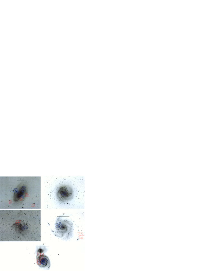
Available HST WFPC2 observations for each galaxy were downloaded from the archive using the “on-the-fly” calibration system, which automatically uses the best reference files for calibration. The WFPC2 pipeline steps include: bad pixel masking, A/D correction, bias and dark subtraction, and flat field correction. The locations of the fields are shown in Figure 1 for each target galaxy. Because we rely on what is available (taken for a host of different projects with a variety of filters, exposure times, etc.), we first briefly summarize basic information for each target galaxy, and then give a general recipe for reduction. Information for the fields used in this work, such as the proposal identification, specific filters and exposure times are compiled in Table 2.

M81 HST WFPC2 observations include seven fields imaged in $UBVI$, three fields imaged in $BVI$, and an 11th outer field with $VI$ imaging (see Table 2 for details). We include this outer field because its large projected distance ($\sim 12.5$ arcmin) along the semi-minor axis makes it unlikely that reddened young clusters reside here, and its location provides a glimpse further out into the halo of this bulge-dominated galaxy than other available multi-filter HST fields. While HST imaging does not provide large coverage in M81, it does allow us to probe deeper than previous ground-based surveys.

For M83, we use a single HST WFPC2 field pointing taken in $UVI$ filters. While this does not provide much coverage beyond the central portions in this galaxy, evidence for an ancient cluster system would be interesting and potentially important for followup observations. NGC6946 has one WFPC2 field imaged in $UBVI$ and a second imaged in $BVI$.

The observations used for M101 were taken between 1994 and 2000 with the WFPC2, and will be described in detail, along with basic data reduction and cluster selection, in an upcoming paper. Here we provide a brief summary. Field 1 was observed in UBVI bands, and field 2 in BVI. Both pointings were taken for the Cepheid Key Distance Project, and hence had enough observations with small, random offsets that we were able to drizzle these images in order to recover resolution from the undersampled WF CCDs.

Observations of M51 and its nearby companion (NGC 5195) were taken for a variety of projects. Field 1 is imaged in UBVI, Field 2 in BVRI with some overlapping U band, and fields 3 and 4 in BVI. NGC 5195 is covered in VI filters; results from this field are discussed in Lee, Chandar, & Whitmore (2004, in prep). Taken together, the five fields cover $\sim 50$% of the two-galaxy system. Details of the reduction will be presented in our upcoming paper, which focuses on the age distribution and other properties of the numerous young massive clusters detected in this interacting system.

In general, for each field and filter combination, available observations were combined in pairs to eliminate cosmic rays, after first checking the alignment. Combined images were corrected for geometric distortion, as described in Holtzman et al.  (1995). For field 7 in M81 the three stepped observations in each of the BVI filters were shifted and combined.

Table 2SUMMARY OF HST WFPC2 FIELD OBSERVATIONS

FIELD	proposid	Filters and Total Exposure Times [sec]
		U	B	V	R	I
M81–1	6139	F336W, 1160	F439W, 1200	F555W, 900	F675W, 900	F814W, 900
M81–2	5480	F336W, 1200	F439W, 600	F555W, 300	F675W, 300	F814W, 300
M81–3	7909	F300W, 3200	F450W, 3100	F606W, 800	$\cdots$	F814W, 800
M81–4	7909	F300W, 7300	F450W, 4300	F606W, 2000	$\cdots$	F814W, 2200
M81–5	9073	$\cdots$	F450W, 2000	F555W, 2000	$\cdots$	F814W, 2000
M81–6	5397	F336W, 1800	F439W, 1200	F555W, 800	$\cdots$	F814W, 800
M81–7	7351	$\cdots$	F439W, 2200	F555W, 1300	$\cdots$	F814W, 1300
M81–8	5397	F336W, 1800	F439W, 1200	F555W, 800	$\cdots$	F814W, 800
M81–9	9634	$\cdots$	F450W, 2000	F606W, 1000	$\cdots$	F814W, 800
M81–10	9086	$\cdots$	$\cdots$	F606W, 5200	$\cdots$	F814W, 5500
M81–11	8061	F300W, 1500	F450W, 5800	F606W, 8700	$\cdots$	F814W, 3000
M83–1	8238	F300W, 2100	$\cdots$	F547M, 930	$\cdots$	F814W, 710
NGC 6946–1	8715	F336W, 3000	F439W, 2200	F555W, 600	$\cdots$	F814W, 1400
NGC 6946–2	9073	$\cdots$	F450W, 2000	F555W, 2000	$\cdots$	F814W, 2000
M101–1	5397	F336W, 1200	F439W, 1100	F555W, 13200	$\cdots$	F814W, 4600
M101–2	5397	$\cdots$	F439W, 1050	F555W, 4200	$\cdots$	F814W, 4800
M51–1	7375	F336W, 1200	F439W, 1100	F555W, 1200	$\cdots$	F814W, 1000
M51–2	5777	F336, 1200	F439W, 1400	F555W, 600	F675W, 600	F814W, 600
M51–3	9073	$\cdots$	F450W, 2000	F555W, 2000	$\cdots$	F814W, 2000
M51–4	9073	$\cdots$	F450W, 2000	F555W, 2000	$\cdots$	F814W, 2000

3.2. Object Detection, Star Cluster Selection, and Photometry

3.2.1 Detection

To identify star clusters, we use morphological information provided by SEXTRACTOR (Bertin & Arnouts 1996), to separate true clusters from contaminants such as individual stars, background galaxies, and blends. SEXTRACTOR performed well in our moderately crowded stellar fields. Detection was run on the V band images (either drizzled or combined) for each field, since in all cases these were the deepest and/or had the best resolution. We used a threshold of $4\sigma$ above the local background level, in order to avoid large numbers of detections of very faint objects in our variable, moderately crowded fields. In addition to the output from SEXTRACTOR, point spread function (PSF) fitting was performed on each object, using the IRAF task ALLSTAR (Stetson 1987). The PSF was created by automatically choosing bright, isolated stars using size, shape, and neighbor information.

3.2.2 Cluster Selection

Cluster candidates were selected to be more extended than the PSF and have low ellipticity values. This eliminated the majority of individual stars, background galaxies, and blends. The primary remaining source of contamination in our cluster catalogs is from blends of a few superposed stars (although a number of these were eliminated from the ellipticity cut). Finally, each object was visually inspected, and blends (which are defined as objects which have large scatter in the central portions relative to the best fit Moffat profile) were eliminated. This pipeline provided final star cluster catalogs in each galaxy. Independent checks by BW and RC in M101 showed that very few ($\sim 8$ out of $\sim 400$) extended objects which appear to be star clusters were missed by this algorithm, particularly at the brighter end. We therefore make the assumption that we are missing a small percentage of clusters to $V\sim 23.0$ in M101, and that our algorithm is similarly successful for the other sample galaxies down to comparable completeness limits (discussed in $\S 3.5.2$).

3.2.3 Photometry

Because how extended clusters appear in HST images depends on both their intrinsic size and galaxy distance, we used somewhat different techniques to select clusters in M81 (the closest galaxy in our sample) from those used on M83, NGC 6946, M101, and M51. For M81, photometry (using the PHOT task in IRAF) was performed on clusters using a 10 pixel radius aperture. For the more distant galaxies, we used a 3 pixel (non-drizzled) radius, in order to minimize the contamination from nearby objects. While this technique provides robust cluster colors (which are negligibly affected by aperture corrections; Holtzman et al.  1995), there is a significant fraction of light outside this radius, which must be corrected for when studying the distribution of total cluster luminosities.

Here, we describe our general technique for deriving approximate aperture corrections, by using M51 as a (representative) example. In order to measure aperture corrections from 3 to 5 pixels (hereafter $\Delta m_{3->5}$) for our extended sources, we identified relatively isolated clusters on the PC CCD and WF CCDs. In general, these objects were typically young star clusters, since young massive clusters tend to be more numerous than ancient clusters in later type spirals. An average, empirical aperture correction was then obtained by measuring the mean magnitude differences in 5 and 3 pixel aperture radii. For M51, we find mean $\Delta m_{3->5}$ values of $-0.290$ and $-0.245$ for the PC and WF CCDs respectively. These values were compared with table 1 of Larsen & Brodie (2000), where they have tabulated aperture corrections based on synthetic King model profiles. We find that our values are slightly smaller than their KING30 profiles (concentration parameter 30), for a synthetic cluster with a typical FWHM value of 1.0 pixels. Overall, we find that M51 clusters have a FWHM of $\sim 0.8$ pixels (Lee, Chandar, & Whitmore, 2004). (The description and results of cluster size measurements is presented in $\S 4.4$.) This gives further confidence in the empirically derived aperture corrections, since our smaller intrinsic cluster size would result in a smaller simulated aperture correction, bringing the two values into excellent agreement. Because very few of the clusters in our M51 GC sample are isolated within a 30 pixel radius, we use table 1 in Larsen & Brodie (2000) to complete the aperture correction to an infinite radius for the WF CCDs, and use 2 isolated sources in our PC images. The final aperture corrections in the PC and WF CCDs for M51 are $-0.39$ and $-0.31$ respectively. However, we note that aperture corrections are strongly dependent on intrinsic object size, and for clusters with sizes as large as 2.0 pixels ($R_{eff}=12~{}\mbox{pc}$) the total V magnitude error will be $\sim 0.7$ magnitudes. Hence it should be kept in mind that our aperture corrections are for a typically sized cluster; individual clusters will vary. We note that this will have a negligible effect on our color estimates, since the same size aperture is used for each bandpass.

The following steps were used to transform measured broadband WFPC2 instrumental magnitudes to Johnson-Cousins $U$, $B$, $V$, $R$ and $I$ magnitudes: (i) the instrumental magnitudes were corrected for the charge-transfer efficiency (CTE) loss, using the prescription given by A. Dolphin (2000; see http://www.noao.edu/staff/dolphin/wfpc2_calib/ for updated calibrated information); (ii) the corrected instrumental magnitudes were converted to standard Johnson-Cousins $U$, $B$, $V$, and $I$ magnitudes. Using Equation 8 and Table 7 of Holtzman et al.  (1995), the magnitudes were derived iteratively using WFPC2 observations in two filters, with all zeropoints substituted from Dolphin (2000), except for the F300W filter (zeropoint for this filter comes from the WFPC2 Handbook). $U$ band magnitudes are taken from the coupling of the $U$ and $B$ filters, $B$ magnitudes from the $B$ and $V$ filter combination, and $V$ and $I$ magnitudes from the $V$ and $I$ filter solution.

We made explicit comparison of the photometry for individual objects presented here with that from previous works in upcoming papers on the young cluster systems of M51 and M101. For M51, a photometric comparison with clusters studied in Larsen (2000) are in good agreement – the mean difference in the V band magnitudes is 0.002, and the mean difference in color $\Delta~{}(B-V)$ is $0.048$, in the sense that our $(B-V)$ color is slightly redder than that given in Larsen (2000). For M101, our comparison with the work of Bresolin et al. (1996) shows larger differences. The mean difference in both V magnitude and color of $\Delta~{}(B-V)$ is $0.066$.

3.3. Cluster Reddening Distribution

3.3.1 Deriving Ages and Reddening for Clusters

The final step is to separate ancient globular cluster candidates from the more numerous young massive clusters found in these galaxies (M81 is the exception, with a higher fraction of luminous, ancient clusters than comparably bright young clusters). Because morphologically young and old clusters are indistinguishable, at this point we used colors to separate them. However, there remains the ambiguity of separating truly ancient, red clusters from young, highly reddened objects. This task becomes much easier when there are a minimum of three broadband filters, particularly including the U bandpass. Here we briefly describe using UBVI observations of field 1 in both M51 and M101 to study the statistics of the $E(B-V)$ distribution of stellar clusters, which provides information on the contamination of our ancient cluster sample from reddened young clusters. The cluster system of NGC 6946 has been studied previously by Larsen (2002). M83 only has UVI filters, making the derived extinction distribution less robust than in M51 and M101.

In order to determine the age and reddening for each cluster, we use a modification of the technique described in detail in Bik et al.  (2003) (the Bik et al.  version of the fitting routine was kindly made available to us by H. Lamers). We compared the observed magnitudes with spectral energy distributions derived from the theoretical evolutionary synthesis models of Bruzual & Charlot (2000; hereafter BC00). These spectral synthesis models are available for a number of metallicities; however, due to the well known age-metallicity-reddening degeneracy in integrated cluster colors, we initially assumed the solar model for comparison with the M51 and M101 clusters, in order to best match the young cluster population. Observations of HII regions in these galaxies establish that the current metallicity of the gas is approximately solar (e.g., Diaz et al. 1991; Hill et al.  1997). Tests establish that this assumption has a negligible effect on the derived ages and extinction values for younger stellar populations ($\leq 1$ Gyr), but preferentially effects the ages estimated for older clusters, where metallicity influences become more pronounced than age influences in the integrated colors. However, since we are only interested in selecting the ancient cluster populations and not in their precise ages (which have to wait for integrated spectroscopy), the integrated colors are sufficient to separate young and old single stellar populations.

Details of the BC00 themselves can be found in (Bruzual & Charlot 1993). Our choice of models assumes that the stars have a Salpeter (1955) initial-mass function (IMF) slope $\frac{d(logN)}{d(logM)}=-2.35$. The lower mass cutoff is $0.1M_{\odot}$ and the upper mass cutoff is $125M_{\odot}$; these limits (particularly the lower mass cutoff) affect the associated $M/L_{V}$ ratios, and thus the cluster mass estimates. For each metallicity, the models span ages from 1 Myr to 15 Gyr.

In order to fit the observed spectral energy distribution of the clusters with the models, we use a standard $\chi^{2}$ minimization technique, where we fit the age and reddening of the cluster simultaneously. For each BC00 model age, we compare the SED to the model reddened by $E(B-V)$ values between 0.0 and 2.0 in steps of 0.02. For every combination of age/extinction, we fit the model to the observed cluster SED, where observations in each filter are weighted by the photometric uncertainty for that particular measurement. Each model/reddening combination results in a $\chi^{2}$ measurement. The fit with a minimum value of $\chi^{2}$ is adopted as the best fit age/$E_{B-V}$ combination. The procedure described above was implemented for all clusters with $UBVI$ imaging.

3.3.2 Cluster Extinction Distributions

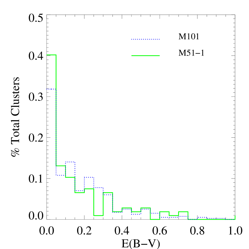
In Figure 2, we show the derived extinction distributions for all M101-1 and M51-1 clusters, regardless of age. We will distinguish between our catalogs containing “all” clusters (regardless of age), and GC candidates, which are a subset of the entire cluster catalog based on color selections. The M101 and M51 $E_{B-V}$ distributions from the age fitting technique described above is (surprisingly) peaked towards low extinction values ($\sim 70$% have less than 0.1), confirming the result found by Bik et al.  (2003) for M51 clusters. This is in sharp contrast to the situation in the Antennae, where we find that the youngest clusters have a mean $E_{B-V}$ value of 0.9. Because young clusters dominate our samples and are most likely to have large reddening, they provide some guidance for typical (upper limits) for the older clusters in each galaxy. Thus it appears unlikely that our ancient cluster samples have significant contamination from highly reddened young clusters.

3.4. Final Globular Cluster Selection

Table 3GLOBULAR CLUSTER CANDIDATES IN M81

#	V	(V$-$I)	(B$-$V)	(U$-$B)	$r_{\mathrm{eff}}$
	(mag)	(mag)	(mag)	(mag)	(pc)
1	$20.649\pm 0.052$	$1.337\pm 0.030$	$1.020\pm 0.098$	$0.117\pm 0.395$	1.5
2	$19.824\pm 0.011$	$1.286\pm 0.012$	$0.957\pm 0.032$	$0.035\pm 0.093$	4.0
3	$21.336\pm 0.061$	$1.250\pm 0.050$	$0.847\pm 0.084$	$0.073\pm 0.309$	2.7
4	$21.377\pm 0.052$	$1.530\pm 0.026$	$1.200\pm 0.076$	$0.399\pm 0.450$	1.5
5	$20.504\pm 0.023$	$1.125\pm 0.019$	$1.018\pm 0.044$	$0.105\pm 0.152$	1.0
6	$19.980\pm 0.016$	$1.197\pm 0.023$	$0.955\pm 0.050$	$0.118\pm 0.175$	14.2
7	$22.073\pm 0.086$	$1.226\pm 0.060$	$0.963\pm 0.123$	$0.268\pm 0.694$	4.4
8	$21.045\pm 0.029$	$1.175\pm 0.026$	$0.920\pm 0.061$	$0.082\pm 0.233$	2.6
9	$20.163\pm 0.014$	$1.376\pm 0.014$	$1.104\pm 0.050$	$0.317\pm 0.137$	2.1
10	$19.694\pm 0.011$	$1.057\pm 0.017$	$0.854\pm 0.044$	$-$$0.149\pm 0.074$	0.9
11	$19.716\pm 0.008$	$1.185\pm 0.015$	$0.905\pm 0.017$	$0.119\pm 0.136$	2.6
12	$20.057\pm 0.018$	$1.089\pm 0.014$	$1.029\pm 0.016$	$\cdots$	1.0
13	$20.432\pm 0.023$	$1.175\pm 0.019$	$0.884\pm 0.019$	$0.097\pm 0.124$	1.3
14	$20.371\pm 0.018$	$1.287\pm 0.018$	$1.021\pm 0.021$	$0.009\pm 0.142$	1.4
15	$19.751\pm 0.012$	$1.325\pm 0.018$	$1.083\pm 0.022$	$0.460\pm 0.246$	11.5
16	$19.347\pm 0.005$	$1.116\pm 0.008$	$0.843\pm 0.012$	$-$$0.160\pm 0.073$	1.8
17	$19.469\pm 0.005$	$1.402\pm 0.011$	$1.003\pm 0.018$	$0.440\pm 0.204$	9.6
18	$18.553\pm 0.005$	$1.396\pm 0.005$	$1.139\pm 0.008$	$0.390\pm 0.051$	2.0
19	$17.580\pm 0.002$	$1.195\pm 0.003$	$0.766\pm 0.004$	$-$$0.127\pm 0.020$	7.2
20	$19.003\pm 0.005$	$1.142\pm 0.006$	$0.927\pm 0.010$	$-$$0.123\pm 0.050$	3.7
21	$19.281\pm 0.009$	$1.343\pm 0.008$	$0.992\pm 0.010$	$0.320\pm 0.064$	1.1
22	$19.805\pm 0.013$	$1.200\pm 0.011$	$1.002\pm 0.015$	$0.085\pm 0.085$	2.3
23	$20.536\pm 0.025$	$1.447\pm 0.035$	$0.965\pm 0.040$	$0.587\pm 0.365$	3.6
24	$22.164\pm 0.029$	$1.397\pm 0.034$	$1.017\pm 0.060$	$\cdots$	1.1
25	$20.942\pm 0.012$	$1.305\pm 0.020$	$1.013\pm 0.033$	$\cdots$	2.7
26	$20.145\pm 0.008$	$1.301\pm 0.011$	$1.132\pm 0.017$	$\cdots$	2.2
27	$21.013\pm 0.023$	$1.188\pm 0.024$	$0.961\pm 0.030$	$\cdots$	3.5
28	$20.684\pm 0.016$	$1.414\pm 0.016$	$1.086\pm 0.024$	$\cdots$	1.4
29	$19.321\pm 0.005$	$1.151\pm 0.008$	$0.882\pm 0.019$	$0.075\pm 0.041$	1.3
30	$19.826\pm 0.008$	$1.521\pm 0.010$	$1.176\pm 0.027$	$0.344\pm 0.077$	0.9
31	$20.247\pm 0.010$	$1.089\pm 0.016$	$0.794\pm 0.035$	$0.083\pm 0.082$	6.5
32	$18.763\pm 0.004$	$1.234\pm 0.006$	$0.986\pm 0.014$	$0.237\pm 0.031$	0.8
33	$20.790\pm 0.011$	$1.324\pm 0.036$	$1.245\pm 0.252$	$\cdots$	19.8
34	$19.997\pm 0.007$	$1.138\pm 0.009$	$0.849\pm 0.024$	$\cdots$	2.2
35	$21.903\pm 0.031$	$1.267\pm 0.038$	$1.258\pm 0.210$	$\cdots$	9.7
36	$21.277\pm 0.019$	$1.307\pm 0.044$	$0.811\pm 0.139$	$\cdots$	8.7
37	$22.389\pm 0.045$	$1.193\pm 0.053$	$0.893\pm 0.176$	$-0.123\pm 0.417$	1.1
38	$20.672\pm 0.016$	$1.302\pm 0.020$	$1.054\pm 0.053$	$0.210\pm 0.149$	7.5
39	$22.230\pm 0.060$	$1.294\pm 0.052$	$1.164\pm 0.171$	$0.694\pm 1.315$	3.0
40	$20.560\pm 0.021$	$1.795\pm 0.021$	$1.527\pm 0.095$	$0.005\pm 0.168$	3.4
41	$21.006\pm 0.022$	$1.179\pm 0.033$	$0.808\pm 0.073$	$1.056\pm 1.306$	23.4
42	$20.894\pm 0.022$	$1.502\pm 0.026$	$1.130\pm 0.076$	$0.349\pm 0.283$	7.7
43	$22.452\pm 0.048$	$1.397\pm 0.054$	$0.912\pm 0.086$	$\cdots$	4.3
44	$20.360\pm 0.010$	$1.932\pm 0.014$	$2.047\pm 0.041$	$\cdots$	1.6
45	$21.941\pm 0.016$	$1.679\pm 0.024$	$\cdots$	$\cdots$	4.6
46	$22.922\pm 0.058$	$1.318\pm 0.054$	$\cdots$	$\cdots$	3.1
47	$22.031\pm 0.029$	$1.306\pm 0.035$	$0.820\pm 0.065$	$\cdots$	5.7

For the final globular cluster selection, we reran our age fitting routine using two additional (lower metallicity) BC00 models: 1/5 solar and 1/50 solar metallicity. Clusters which were best fit by ages $\sim 9.4$ (log) yrs and older in any of these models were selected as globular cluster candidates. Based on the results of the SED fitting technique, we find that the following colors can be used as a reasonable selection criterion for globular clusters when UBVI photometry is available: $V-I\geq 0.7$, $B-V\geq 0.55$, and $U-B\geq-0.15$, although there is some variation in the exact values, depending upon the actual metallicity of the cluster. If only $BVI$ photometry is available, we use a slightly more stringent color combination $V-I\geq 0.8$, and $B-V\geq 0.55$, and if only $VI$ is available (this is the case for only one field in the halo of M81), we use $V-I\geq 0.8$. Many of the fields used in this study revealed almost no background galaxies, suggesting that these spiral disks are relatively opaque (M81 is an exception). Because we were able to eliminate the few observed galaxies on the basis of their morphology, we did not make a color cut at the red end.

In the next section we quantify the expected contamination from inclusion of reddened young clusters in fields with only $BVI$ photometry. Note that for the objects discussed here to actually be reddened young clusters rather than ancient star clusters, their $E(B-V)$ values would have to be between $\sim 0.4-0.8$, which is found for extremely few resolved objects in our “all cluster” catalogs. Finally, the location of the GC candidates were visually inspected to make sure they did not fall in the center of a spiral arm, which would significantly increase the probability that a given object could be a reddened YMC rather than ancient GCs. Three such candidates (with BVI photometry) were removed from our ancient cluster catalog in M51. Our final GC catalogs, along with photometric measurements are presented in Tables $3-7$.

Table 4GLOBULAR CLUSTER CANDIDATES IN M83

#	V	(V$-$I)	(U$-$V)	$r_{\mathrm{eff}}$
	(mag)	(mag)	(mag)	(pc)
1	$20.833\pm 0.034$	$1.157\pm 0.048$	$0.738\pm 0.121$	1.2
2	$19.666\pm 0.016$	$1.135\pm 0.027$	$0.937\pm 0.059$	2.8
3	$18.266\pm 0.007$	$1.140\pm 0.010$	$1.236\pm 0.031$	1.0
4	$17.258\pm 0.004$	$1.065\pm 0.006$	$0.943\pm 0.016$	1.1
5	$19.217\pm 0.010$	$1.800\pm 0.012$	$2.583\pm 0.128$	1.1
6	$16.383\pm 0.005$	$1.441\pm 0.006$	$1.363\pm 0.016$	2.1
7	$21.094\pm 0.031$	$1.436\pm 0.038$	$1.633\pm 0.328$	2.3
8	$21.798\pm 0.050$	$1.441\pm 0.062$	$1.854\pm 0.793$	6.4
9	$21.005\pm 0.037$	$1.785\pm 0.044$	$2.947\pm 0.801$	2.4
10	$22.069\pm 0.067$	$1.167\pm 0.093$	$1.674\pm 0.703$	1.9
11	$21.653\pm 0.050$	$1.748\pm 0.059$	$2.063\pm 0.662$	1.9
12	$21.042\pm 0.032$	$1.148\pm 0.043$	$0.861\pm 0.164$	4.8
13	$20.410\pm 0.029$	$1.019\pm 0.043$	$1.215\pm 0.149$	11.4
14	$20.956\pm 0.034$	$1.265\pm 0.044$	$1.312\pm 0.221$	6.6
15	$20.717\pm 0.034$	$1.152\pm 0.047$	$1.284\pm 0.168$	4.3
16	$20.247\pm 0.026$	$1.419\pm 0.033$	$2.430\pm 0.284$	4.3
17	$20.772\pm 0.042$	$1.400\pm 0.053$	$1.076\pm 0.149$	4.6
18	$21.033\pm 0.034$	$1.359\pm 0.047$	$1.348\pm 0.206$	1.8
19	$21.535\pm 0.046$	$1.062\pm 0.060$	$1.092\pm 0.341$	5.0
20	$19.295\pm 0.011$	$1.335\pm 0.014$	$0.978\pm 0.051$	1.7
21	$20.704\pm 0.025$	$1.318\pm 0.031$	$1.316\pm 0.161$	8.1

HST studies of GC systems in ellipticals, lenticulars, and edge-on spiral galaxies suggest possible variation in the intrinsic GC color beyond that seen in the M31 and MW systems. For example, Goudfrooij et al.  (2003) detected cluster candidates in the halos of edge-on spirals with significantly bluer colors. They find that NGC 4517 has a relatively large number of GC candidates with $0.3\leq V-I\leq 0.6$; spectroscopy is needed to confirm whether these are actually ancient clusters associated with the host galaxy. Such objects would not be retained as cluster candidates in our study, as their colors imply a significantly younger age.

Table 5GLOBULAR CLUSTER CANDIDATES IN NGC 6946

#	V	(V$-$I)	(B$-$V)	(U$-$B)	$r_{\mathrm{eff}}$
	(mag)	(mag)	(mag)	(mag)	(pc)
1	$20.854\pm 0.019$	$1.556\pm 0.024$	$0.951\pm 0.045$	$0.119\pm 0.130$	2.3
2	$22.245\pm 0.045$	$1.768\pm 0.056$	$1.063\pm 0.140$	$0.360\pm 0.674$	2.6
3	$21.104\pm 0.0204$	$1.895\pm 0.023$	$1.391\pm 0.074$	$0.199\pm 0.243$	3.1
4	$21.771\pm 0.029$	$1.717\pm 0.034$	$1.265\pm 0.116$	$\cdots$	1.3
5	$21.367\pm 0.023$	$1.777\pm 0.028$	$1.337\pm 0.092$	$\cdots$	3.9
6	$22.000\pm 0.020$	$1.524\pm 0.025$	$1.237\pm 0.050$	$\cdots$	2.4
7	$17.688\pm 0.003$	$1.562\pm 0.004$	$1.170\pm 0.006$	$\cdots$	1.4
8	$23.136\pm 0.044$	$1.442\pm 0.054$	$1.149\pm 0.107$	$\cdots$	2.0
9	$22.162\pm 0.022$	$1.330\pm 0.028$	$1.023\pm 0.048$	$\cdots$	2.6
10	$23.452\pm 0.053$	$1.575\pm 0.065$	$1.004\pm 0.123$	$\cdots$	2.9
11	$23.150\pm 0.038$	$1.509\pm 0.047$	$1.367\pm 0.108$	$\cdots$	7.3
12	$23.183\pm 0.040$	$1.338\pm 0.051$	$0.978\pm 0.092$	$\cdots$	8.9
13	$22.196\pm 0.028$	$1.559\pm 0.034$	$1.268\pm 0.067$	$\cdots$	8.0
14	$22.770\pm 0.057$	$1.725\pm 0.065$	$1.263\pm 0.131$	$\cdots$	3.5
15	$23.141\pm 0.069$	$1.383\pm 0.088$	$1.027\pm 0.141$	$\cdots$	1.0
16	$21.687\pm 0.027$	$1.546\pm 0.033$	$1.252\pm 0.057$	$\cdots$	1.3
17	$23.394\pm 0.082$	$1.471\pm 0.101$	$0.979\pm 0.159$	$\cdots$	1.9
18	$23.009\pm 0.041$	$1.494\pm 0.051$	$1.025\pm 0.090$	$\cdots$	8.6
19	$21.151\pm 0.013$	$1.290\pm 0.017$	$1.027\pm 0.028$	$\cdots$	3.0

3.5. Completeness and Contamination Estimates

3.5.1 Contamination

Potential contaminants to our globular cluster catalogs are: individual stars, background galaxies, blends, and reddened young massive clusters. We have eliminated individual stars by requiring that GC candidates be resolved. Background galaxies have been mostly eliminated based on morphology, which is possible with the excellent resolution provided by HST imaging. There are two additional reasons we believe that our cluster samples are essentially free of faint background galaxies. The first reason applies to the later-type spirals in our sample. In the central portions of these galaxies, where the density of GCs is expected to be highest, the disks appear to be nearly opaque. For example, two of us (BCW and RC) attempted to locate background galaxies in field M101$-$1, and discovered that almost no such objects were visible in the entire WFPC2 field of view. This contrasts with the situation for the earliest-type spiral, M81, where background galaxies are clearly visible in all fields used in this work. However, because few background elliptical galaxies are expected to be as luminous as the majority of GCs at the distance of M81, we expect little to no contamination. This conclusion is supported by ground-based spectra of M81 GCs selected from these HST fields (from the Chandar, Ford, & Tsvetanov 2001 catalog), where we find no background galaxies to $V\sim 20$. Blends and reddened YMCs may be a more significant problem. We have eliminated all obvious blends based on a final visual inspection; however a few closely blended objects may still remain.

Table 6GLOBULAR CLUSTER CANDIDATES IN M101

#	V	(V$-$I)	(B$-$V)	(U$-$B)	$r_{\mathrm{eff}}$
	(mag)	(mag)	(mag)	(mag)	(pc)
1	$22.562\pm 0.013$	$1.070\pm 0.060$	$0.989\pm 0.056$	$0.535\pm 0.392$	3.5
2	$23.350\pm 0.028$	$1.120\pm 0.040$	$0.919\pm 0.114$	$0.377\pm 0.649$	5.0
3	$23.249\pm 0.044$	$1.148\pm 0.056$	$1.051\pm 0.151$	$0.065\pm 0.430$	3.5
4	$21.540\pm 0.009$	$1.087\pm 0.0130$	$0.823\pm 0.037$	$0.0350\pm 0.086$	3.4
5	$23.271\pm 0.046$	$0.955\pm 0.064$	$0.518\pm 0.102$	$0.303\pm 0.408$	4.4
6	$23.205\pm 0.023$	$1.319\pm 0.031$	$0.927\pm 0.107$	$0.330\pm 1.210$	8.3
7	$23.478\pm 0.028$	$1.309\pm 0.038$	$0.726\pm 0.113$	$\cdots$	5.0
8	$20.821\pm 0.003$	$1.895\pm 0.004$	$1.494\pm 0.037$	$0.374\pm 0.123$	9.4
9	$22.206\pm 0.011$	$1.271\pm 0.014$	$0.889\pm 0.055$	$\cdots$	3.3
10	$22.587\pm 0.014$	$1.501\pm 0.018$	$1.103\pm 0.087$	$\cdots$	7.5
11	$22.132\pm 0.013$	$1.260\pm 0.017$	$0.686\pm 0.050$	$0.026\pm 0.129$	4.8
12	$23.084\pm 0.023$	$1.010\pm 0.033$	$0.602\pm 0.083$	$0.115\pm 0.347$	9.2
13	$22.368\pm 0.011$	$0.994\pm 0.017$	$0.549\pm 0.046$	$0.353\pm 0.190$	5.9
14	$20.027\pm 0.002$	$1.225\pm 0.003$	$0.859\pm 0.016$	$0.140\pm 0.040$	4.1
15	$20.983\pm 0.004$	$1.288\pm 0.006$	$0.894\pm 0.027$	$0.241\pm 0.083$	2.5
16	$23.096\pm 0.015$	$0.774\pm 0.030$	$0.622\pm 0.070$	$0.598\pm 0.556$	3.6
17	$22.081\pm 0.010$	$1.13\pm 0.013$	$0.665\pm 0.042$	$0.228\pm 0.142$	3.8
18	$22.456\pm 0.008$	$0.893\pm 0.015$	$0.647\pm 0.050$	$0.156\pm 0.164$	9.1
19	$23.642\pm 0.027$	$0.834\pm 0.046$	$0.510\pm 0.097$	$-0.042\pm 0.287$	2.7
20	$23.893\pm 0.028$	$1.083\pm 0.047$	$0.770\pm 0.137$	$\cdots$	3.7
21	$21.957\pm 0.006$	$0.750\pm 0.012$	$0.524\pm 0.036$	$0.001\pm 0.089$	8.0
22	$23.635\pm 0.034$	$0.968\pm 0.051$	$0.517\pm 0.111$	$-0.048\pm 0.340$	3.5
23	$23.597\pm 0.022$	$1.290\pm 0.030$	$0.723\pm 0.118$	$0.028\pm 0.797$	8.7
24	$23.174\pm 0.015$	$1.283\pm 0.021$	$0.621\pm 0.080$	$0.170\pm 0.653$	6.3
25	$23.280\pm 0.016$	$0.940\pm 0.026$	$0.623\pm 0.086$	$\cdots$	3.7
26	$23.466\pm 0.027$	$1.185\pm 0.036$	$0.516\pm 0.106$	$0.093\pm 0.640$	6.3
27	$22.480\pm 0.015$	$0.978\pm 0.021$	$0.580\pm 0.059$	$0.198\pm 0.247$	6.9
28	$20.405\pm 0.003$	$1.599\pm 0.004$	$1.463\pm 0.030$	$0.269\pm 0.083$	6.8
29	$21.574\pm 0.006$	$1.184\pm 0.008$	$0.724\pm 0.035$	$0.097\pm 0.093$	10.6

Table 7GLOBULAR CLUSTER CANDIDATES IN M51

#	V	(V$-$I)	(B$-$V)	(U$-$B)	$r_{\mathrm{eff}}$
	(mag)	(mag)	(mag)	(mag)	(pc)
1	$21.271\pm 0.022$	$0.974\pm 0.029$	$0.634\pm 0.058$	$-$$0.122\pm 0.148$	12.7
2	$21.384\pm 0.020$	$1.045\pm 0.028$	$0.640\pm 0.056$	$0.348\pm 0.287$	5.2
3	$21.696\pm 0.030$	$0.889\pm 0.040$	$0.647\pm 0.080$	$0.250\pm 0.327$	6.3
4	$21.727\pm 0.028$	$0.816\pm 0.043$	$0.623\pm 0.080$	$-$$0.006\pm 0.220$	9.3
5	$21.252\pm 0.021$	$1.092\pm 0.027$	$0.842\pm 0.065$	$0.085\pm 0.194$	8.5
6	$22.439\pm 0.102$	$1.038\pm 0.132$	$0.707\pm 0.196$	$\cdots$	16.3
7	$21.357\pm 0.041$	$1.053\pm 0.053$	$0.659\pm 0.079$	$-$$0.110\pm 0.165$	4.7
8	$21.412\pm 0.029$	$0.973\pm 0.038$	$0.739\pm 0.077$	$-$$0.083\pm 0.191$	11.3
9	$22.181\pm 0.069$	$0.872\pm 0.108$	$0.600\pm 0.135$	$\cdots$	4.2
10	$22.278\pm 0.029$	$0.928\pm 0.040$	$0.584\pm 0.052$	$\cdots$	3.7
11	$20.424\pm 0.009$	$0.980\pm 0.013$	$0.694\pm 0.017$	$\cdots$	3.9
12	$21.505\pm 0.018$	$1.339\pm 0.022$	$1.027\pm 0.038$	$\cdots$	5.2
13	$23.004\pm 0.042$	$1.172\pm 0.055$	$0.756\pm 0.082$	$\cdots$	20.7
14	$20.294\pm 0.016$	$1.147\pm 0.020$	$0.759\pm 0.027$	$\cdots$	5.5
15	$21.687\pm 0.039$	$0.776\pm 0.059$	$0.659\pm 0.065$	$\cdots$	7.1
16	$21.576\pm 0.021$	$1.090\pm 0.028$	$0.773\pm 0.039$	$\cdots$	13.8
17	$22.066\pm 0.079$	$1.078\pm 0.109$	$0.826\pm 0.133$	$\cdots$	7.2
18	$21.657\pm 0.056$	$1.114\pm 0.067$	$0.751\pm 0.095$	$\cdots$	9.1
19	$22.638\pm 0.029$	$0.878\pm 0.042$	$0.694\pm 0.058$	$\cdots$	12.8
20	$22.429\pm 0.043$	$0.841\pm 0.058$	$0.666\pm 0.076$	$\cdots$	9.5
21	$22.742\pm 0.039$	$1.067\pm 0.053$	$0.658\pm 0.072$	$\cdots$	6.5
22	$23.097\pm 0.036$	$0.845\pm 0.053$	$0.559\pm 0.070$	$\cdots$	7.1
23	$21.954\pm 0.039$	$0.812\pm 0.057$	$0.677\pm 0.063$	$\cdots$	4.4
24	$21.431\pm 0.019$	$0.877\pm 0.028$	$0.576\pm 0.033$	$\cdots$	4.3
25	$22.482\pm 0.052$	$0.813\pm 0.076$	$0.664\pm 0.085$	$\cdots$	5.7
26	$22.368\pm 0.028$	$1.504\pm 0.035$	$1.197\pm 0.066$	$\cdots$	8.7
27	$21.438\pm 0.014$	$0.916\pm 0.021$	$0.709\pm 0.028$	$\cdots$	8.4
28	$22.806\pm 0.037$	$1.479\pm 0.045$	$0.975\pm 0.078$	$\cdots$	9.5
29	$21.937\pm 0.033$	$0.975\pm 0.043$	$0.590\pm 0.069$	$\cdots$	12.0
30	$22.610\pm 0.030$	$1.095\pm 0.041$	$0.738\pm 0.058$	$\cdots$	7.5
31	$23.373\pm 0.045$	$1.119\pm 0.060$	$0.583\pm 0.090$	$\cdots$	7.0
32	$23.409\pm 0.063$	$0.744\pm 0.090$	$0.632\pm 0.125$	$\cdots$	3.6
33	$23.629\pm 0.076$	$1.219\pm 0.110$	$0.913\pm 0.141$	$\cdots$	11.9
34	$20.837\pm 0.070$	$1.252\pm 0.098$	$0.839\pm 0.100$	$\cdots$	2.3

Because some of our ancient clusters were selected from $BVI$ photometry (when no U band imaging was available), there is likely some contamination by reddened young clusters which cannot be sorted out from ancient objects when only these three filters are available. Here, we use the available UBVI imaging in each galaxy to estimate the number of potential (reddened) young clusters in our sample. We used the following technique: clusters which would be selected as GCs according to the BVI color criteria given in $\S 3.4$, were compared with the fraction selected using our UBVI criteria. The fraction of clusters which are clearly young and reddened based on UBVI is assumed to hold for the rest of our GC catalog. For M51-1, we find that (for objects brighter than 21.7), only 1 out of 7 has colors consistent with a highly reddened YMC rather than an ancient GC. Since field 1 covers inner and spiral arm regions, the cluster reddening distribution might reasonably be expected to be representative for the rest of the galaxy, if not an overestimate. Out of 34 total GC candidates in M51, seven have U band photometry. If 1/7 of those with only BVI photometry are expected to be reddened young clusters, we expect $\sim 4$ contaminants in our M51 cluster sample. In M81, an examination of our entire cluster catalog shows a contamination fraction of $\sim 20$% for our GC sample (mostly at the faint end), resulting in an estimated $\sim 4$ reddened young cluster contaminants. In M101, only four of the 29 GC candidates have no U band measurement (due to faintness). For the brighter portion of the sample, we found that $\sim 1$ out of 5 clusters which had BVI colors typical of ancient clusters were actually reddened young clusters. Thus statistically we expect a maximum of one M101 sample clusters to be young. Photometry of all clusters in NGC 6946-2 suggests that no young clusters are in our GC catalog.

3.5.2 Completeness

The completeness of our sample will depend upon a number of complex issues. Completeness in terms of cluster size is one issue, since we have only included resolved objects in this study. In general, we can be reasonably confident that an object is extended if its FWHM is about 0.2 pixels larger than the stellar PSF. At the target galaxy distances, this 0.2 pixel lower size limit corresponds to an effective radius of 0.5, 0.6, 0.9, 1.1, and 1.2 pc for M81, M83, NGC 6946, M101, and M51 respectively. This can be compared with the Galactic GC system to get a very approximate idea of completeness based on size, if the GC systems in these galaxies have similar $r_{eff}-\mbox{galactocentric}$ distance distributions as their Milky Way counterparts. We use the McMaster list (Harris 1996) to estimate the number of Milky Way clusters which would fall out of our samples based on their compactness and photometric properties. Seven Galactic GCs have half mass radii ($r_{\frac{1}{2}}$) smaller than 1.1 pc, and nine have $r_{\frac{1}{2}}\leq 1.2$. However, these Galactic GCs have integrated luminosities of $M_{V}\sim-4~{}\mbox{to}-7$, and so are fainter than the expected GC turnover. Assuming that any missing, compact clusters in our target galaxies follow a similar pattern, the technique used to estimate the total number of GCs (described in $\S 4.5.1$) should not be affected. Thus, we do not make any correction for our inability to detect the most compact clusters.

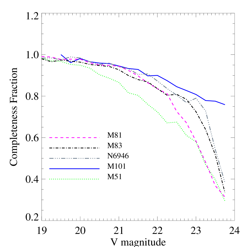
Because of the complicated and often messy spiral regions, and because our detection algorithm requires a final “by eye” check, it is not easy to exactly quantify our completeness levels. We assume that our detection algorithm recovers all resolved clusters (a thorough and independent inspection of clusters in M101 by both R.C. and B.W. suggests that this is a reasonable assumption), even though it may leave in a few blends. Artificial cluster experiments were performed by adding artificial GCs (generated from the ADDSTAR task in IRAF, where instead of stars, clusters were selected) to our images, and then rerunning these through the automated portion of our detection algorithm. These ’fake’ clusters were added in groups of 50 in randomly placed positions on each chip, and then detected and re-photometered. We assume that as long as a GC made it through the automated pipeline, it was not thrown out during the visual inspection phase (which was used primarily to weed out blends). In Figure 3 we show average V band completeness functions for the photometry of GC candidates in each galaxy. Formal completeness levels are likely somewhat optimistic, since the synthetic clusters have been created from previously identified clusters in each field. As expected from the total V band exposure times, the M101 data has a higher completeness level at a given magnitude than the other target galaxies.

4. Results: Globular Cluster System Properties

4.1. Color and Luminosity Distributions

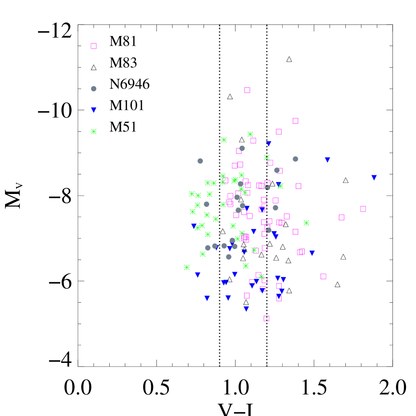
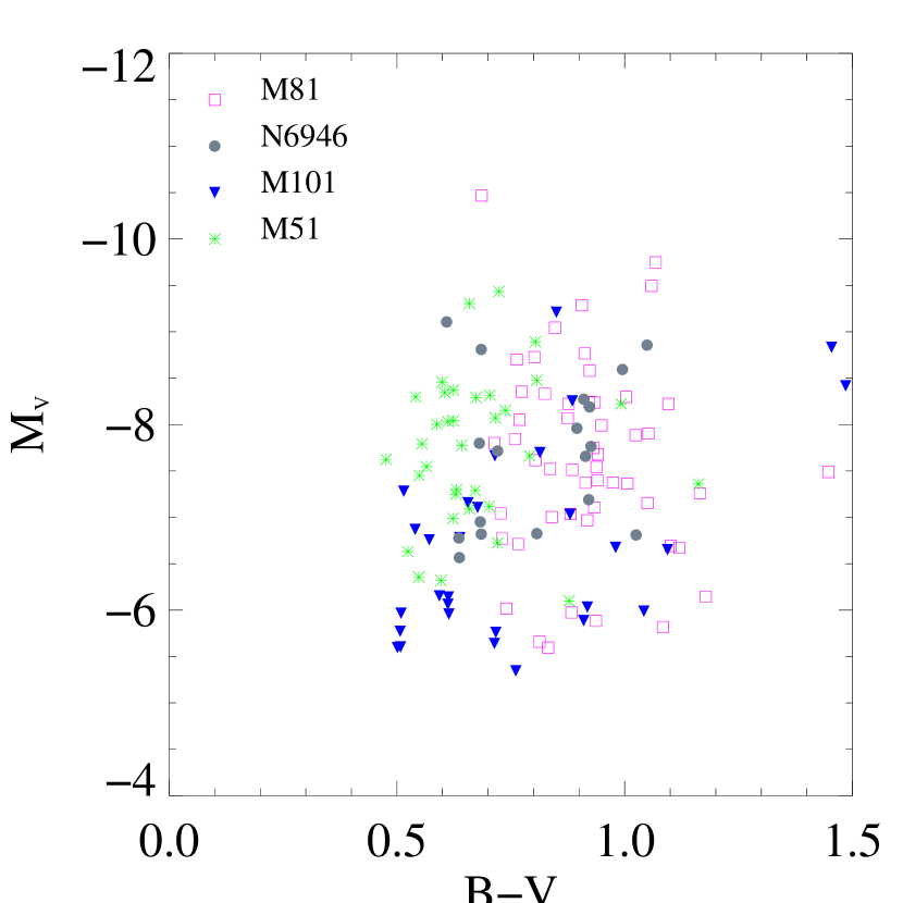
Figure 4 shows the $(V-I)$ vs. $V$ and $(B-V)$ vs. $V$ color magnitude diagrams (CMD) of our detected globular cluster samples. Colors have been dereddened by the foreground extinction values and magnitudes corrected for foreground extinction and distance. In Figure 4a, we show the mean $(V-I)$ colors of the two peaks found for GC systems in many elliptical and lenticular galaxies, at typical values of 0.9 (blue, metal poor) and 1.2 (red, metal rich) (Kundu & Whitmore 2001). Below, we discuss the global luminosity and color distributions for the GC systems in our spiral sample.

One of the most striking features in Figures 4a,b is that the globular clusters from different galaxies appear to separate in color space. The M51 cluster population has mean (foreground reddening corrected) $(B-V)$ and $(V-I)$ colors of 0.67 and 0.95, with standard deviations of 0.14 and 0.17 respectively. Comparable values for the M81 GC sample are 0.92 and 1.19, with standard deviations of 0.15 and 0.18. The mean $(V-I)$ color of the M51 GC system is remarkably similar to the blue (metal-poor) peak found in elliptical and lenticular galaxies (e.g., Burgarella, Kissler-Patig, & Buat 2001), and the mean $(V-I)$ color of our M81 GC sample is remarkably similar to the red (metal-rich) peak in these early type galaxies. The M83 system has a mean $(V-I)$ color of 1.22 with a standard deviation of 0.23 – similar to the metal-rich peak in early type galaxies, but with a large spread. Note that this is primarily due to a number of clusters fainter than $M_{V}\sim-7$, which have predominantly red colors.

Because colors are sensitive to metallicity in single stellar populations older than a few Gyr, the GC color distributions seem to suggest that M51 has a nearly exclusive metal-poor GC population, despite being of a similar Hubble type as the Milky Way, which is known to have formed $\sim 40-50$ GCs more metal rich than $\mbox{[Fe/H]}\sim-1$ (see compilation in Harris 1996). The color distributions for M81 GCs however, are redder, suggesting the presence of metal-rich GCs (although internal reddening would shift any affected cluster to bluer colors). The color distributions are explored further in the next two sections.

In Figure 5 we show the observed V band luminosity distributions for our globular cluster samples, uncorrected for completeness. The dashed lines represent average 80% completeness limits, as discussed in section 3.5.2. Note that these are not the completeness as a function of local background level, and that a single value for each galaxy cannot capture the complicated issue of completeness. For M81, the closest and earliest type spiral in our sample, we see a peak in the GC luminosity function more luminous than the completeness level. This is the characteristic shape and turnover seen in the Milky Way, M31 and most elliptical and lenticular GC systems. Thus M81 GCs appear to have a shape similar to the now familiar “universal” GC luminosity function. While our M83 sample does not contain a large number of GCs, the luminosity function for these objects is similar to that for M81.

M51 is the most distant galaxy in our sample, and does not have extremely deep exposures. Therefore the completeness limit for this galaxy does not quite reach the turnover in the GC luminosity function (which is expected to occur near $M_{V}\sim-7.4$). The apparent peak in the cluster luminosity distribution around $M_{V}\sim-8.5$, is likely caused by one or two effects: 1) variable completeness limits as a function of background level, or 2) possible contamination from reddened young clusters, and is likely not real.

The situation in M101 appears to be quite different from that in M81. While the number of clusters is few, and based primarily on a single HST WFPC2 pointing located near the center, our deep drizzled observations reveal a population of faint, red clusters, which appear to have a powerlaw luminosity distribution down to our completeness limit ($M_{V}\sim-6$). We remind the reader that all of these objects are resolved, so cannot be individual stars. The colors for these faint objects are indistinguishable from the more luminous clusters in our sample (although due to their faintness, the U band photometry has higher uncertainty). The nature of these faint, red clusters is discussed further in $\S 5.1$. Although the GC catalog for NGC 6946 contains relatively few objects, we note that the luminosity distribution appears more similar to that for M101 GCs rather than M81 GCs, due to the apparent “excess” of clusters beyond the expected turnover of $M_{V}\sim-7.4$.

Low number statistics may play a role in the observed luminosity distributions for M101 and NGC 6946. We quantified this effect by performing a simple experiment. A parent gaussian distribution with a peak at $M_{V}=-7.4$ and a width, $\sigma=1.2$ (mimicking fits to the Galactic GC system distribution) was assumed. We imposed a cutoff of $M_{V}=-6$, roughly the 50% completeness limit for NGC 6946, according to Figure 3. This truncated Gaussian was then randomly sampled 19 times, and the resulting distribution of luminosities displayed in a histogram, similar to those shown in Figure 5. We find that roughly $\sim 1/3$ of the time, a distribution somewhat similar to the GCLF for NGC 6946 results, and $\sim 2/3$ of the time the distribution has more clusters near the peak magnitude. Repeating this experiment using a collection of 29 clusters and comparing with the distribution plotted for M101, a similar distribution with excess faint clusters resulted only $5-10$% of the time. Therefore, there is a $90-95$% probability that the M101 GC luminosity function differs substantially from that observed in the Milky Way and a number of other galaxies.

4.2. Color-Color Distributions

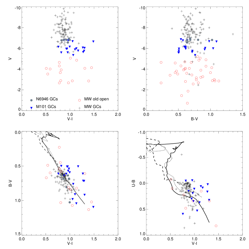
The metallicity distributions of GC systems shed light on the formation history of the parent galaxy. For the GC systems in elliptical galaxies, widespread bimodality in the color (and by extension metallicity) distributions, has helped constrain the most likely formation scenarios for early-type galaxies (e.g., Kundu & Whitmore 2001). However, less is known concerning the metallicity distributions of GC systems in spirals. The two best studied spirals, the Galaxy and M31, both have bimodal GC metallicity distributions (e.g., Cote 1999; Perrett et al.  2002).

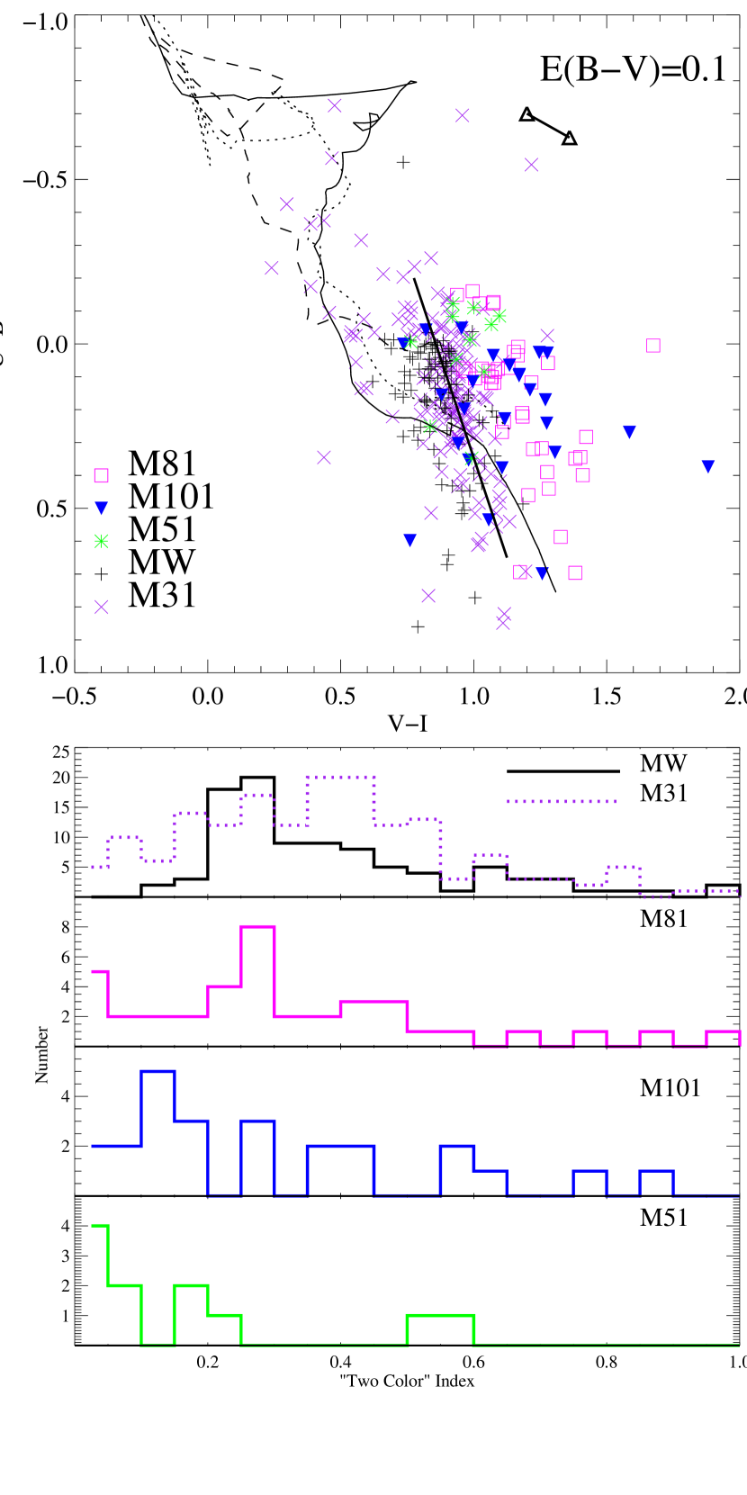
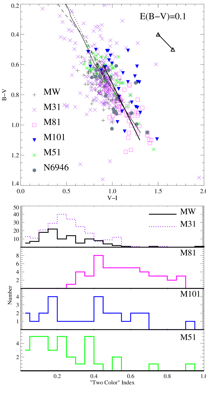
In Figure 6, we plot the cluster $(V-I)$ vs. $(U-B)$ color-color distributions. The GC candidates have been dereddened by foreground $E_{B-V}$ only. These are compared with three different metallicity stellar evolutionary BC00 models: solar (solid line), 1/5 solar (dotted line) and 1/50 solar (dashed line); clearly more metal-rich models have redder colors for ancient populations. For comparison, we also plot the colors of Galactic GCs (Harris 1996) and $\sim 170$ M31 GCs (with UBVI photometry) presented in Barmby et al. (2000). These have been corrected for both foreground and internal extinction (P. Barmby kindly made the derived $E_{B-V}$ values for M31 GCs available to us), for clusters where the $E_{B-V}$ derivation is robust, and by only the foreground value when it is not. We note that there is some scatter in the M31 GC colors, most notably from a handful of blue objects. These are likely young, massive clusters found in the disk of the Andromeda galaxy, as spectroscopically confirmed by Barmby et al.  (2000).

Blue Galactic GC colors agree well with the models, while the redder ones appear to have colors which are offset (blueward) from the high metallicity model predictions of BC00. The dereddened M31 GC colors agree well with their Milky Way counterparts. The M81 GCs presented here however, appear to lie along a different locus than both Milky Way and M31 GCs. Potentially, this is due to internal reddening, which we have not corrected for. We find that if M31 GC colors are only corrected for foreground reddening, they lie in the same region as the M81 GCs, indicating that internal reddening is a plausible explanation for the offset. A second factor supporting the possibility that differential reddening is responsible for the offset between M81 and dereddened M31 GC colors is the location of our M81 fields, which are scattered mostly along the spiral arms and disk. M51 and M101 clusters follow the intrinsic Galactic and M31 GC color-color locus more closely.

We attempt to use the color-color distributions to study the underlying metallicity distribution in spiral GC systems in two ways. First, because the intrinsic colors of Galactic and M31 GCs are in good agreement, we assume that these provide a fiducial for the clusters studied in this work. Figure 6a shows a linear fit to intrinsic M31 GC colors in $(V-I)$ vs. $(U-B)$ color-color space [equation: $(U-B)$ = $3.33\times(V-I)$-2.9]. We assume that deviations from this line are due to internal reddening for the GCs presented in this work, and track them along the reddening vector until they intersect the best fit line, assuming the $R_{V}=3.1$ extinction curve of Cardelli, Clayton, & Mathis (1989). We note that Barmby et al.  (2000) found little difference in the extinction law between Galactic GCs and their M31 counterparts, and we assume the Galactic extinction law is also similar for the galaxies studied in this work. Once we dereddened M81, M101, and M51 GCs, we determined the position of each point along the best fit line; hereafter we refer to this value as the “two color index”. The dereddened measurements in color-color space of ancient star clusters should reflect the underlying metallicity distribution. Histograms of the two color indices for each galaxy sample are shown below the color-color diagram.

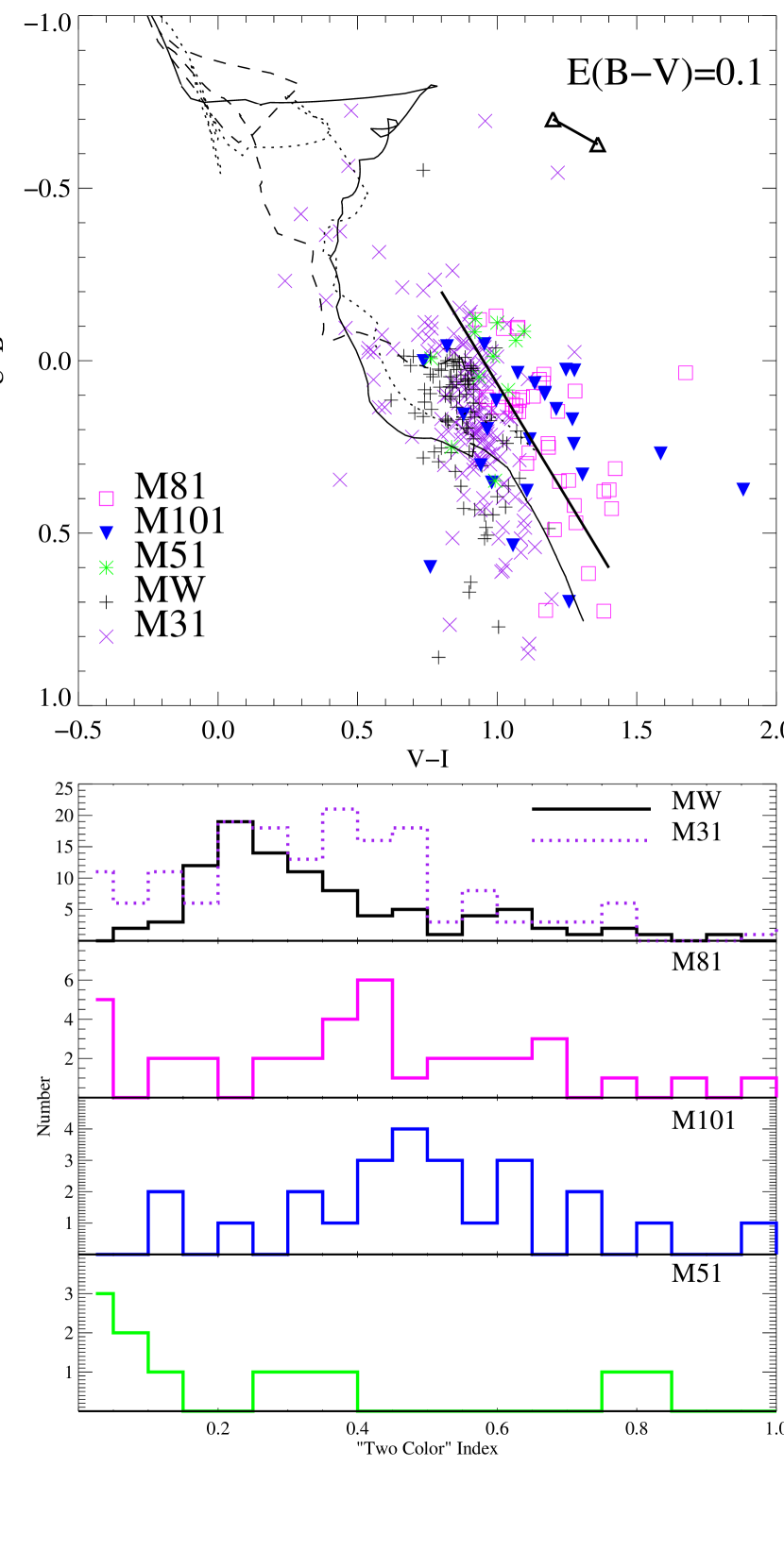
A second possibility is that the M81 GCs in our spiral sample have different intrinsic colors than those in the Galaxy and M31. To explore this possibility, we fit the locus of the M81 GCs in Figure 6b. We then determined the two color index for each object by finding the location of the perpendicular bisector for each cluster. The resulting histograms for Galactic, M31, M81, M101, and M51 GCs are shown in the lower panel of Figure 6b.

In Figures 7a,b we show two other color-color combinations. In Figure 7a, which includes most of the clusters in our sample, we see that four M51 GCs (about 12%) are located in the red GC parameter space, while the rest are consistent with bluer GC colors. This represents an upper limit to the total number of metal-rich GCs in our M51 sample (since any intrinsic reddening would move these objects to bluer colors).

4.3. Color/Metallicity Distributions of GC systems in spirals

Table 8STATISTICS OF COLOR-COLOR DISTRIBUTIONS FOR GC SYSTEMS

	$(U-B)$ v. $(V-I)$			$(U-V)$ v. $(V-I)$
Galaxy	mean	$\sigma$		mean	$\sigma$
Milky Way	0.38 (0.02)	0.19		…	…
M31	0.38 (0.02)	0.22		0.56 (0.05)	0.30
M81	0.33 (0.04)	0.27		0.50 (0.02)	0.29
M101	0.31 (0.06)	0.25		0.48 (0.05)	0.37
M51	0.17 (0.06)	0.18		0.34 (0.07)	0.24

Note. — Mean and standard deviations are calculated for intrinsic (dereddened) two color indices. The technique used to measure this index is described in $\S 4.2$. The values in parentheses give uncertainties in the mean, calculated as $\sigma/\sqrt{N}$

In this section, we attempt to more fully quantify the metallicity distributions of spiral GC systems, by using the two color index developed above. The intrinsic metallicity distributions for M31 and Galactic GCs are known to be bimodal. This translates into an extended color distribution in the lower panels of Figures 6 and 7, including both metal-poor (blue) and metal-rich (red) GCs. In our cluster samples, low numbers also compromise our ability to clearly detect bimodality; because of these small numbers, in general we will refer to “extended” metallicity distributions rather than bimodal distributions. One way to understand the underlying metallicity distribution from colors is to compare statistics between systems in different galaxies. In Table 8, we compile the mean and standard deviation for GC two color indices. These only include clusters with U band photometry, since we are interested in the intrinsic color distributions. We find that the mean and $\sigma$ of the M81 GC system (0.33 and 0.27 respectively) are very similar to those for M31 (0.38 and 0.22) and the Milky Way (0.38 and 0.19). M51 has a significantly lower mean value (0.17) and smaller spread (0.18) than the other three galaxies.

Assuming that the M51 clusters studied here are ancient, this is indicative of lower overall metallicity for the M51 GC system. Although it is possible that the M51 GC candidates are younger and therefore more metal-rich, a comparison with stellar evolutionary models indicates that they would have to be substantially younger than 12 Gyr for this to be true. For example, in the $U-B$ versus $V-I$ color-color diagram shown in Figure 6a, the M51 globular candidates are consistent with the blue, metal-poor M31 and Milky Way GC colors. If these were metal-rich the only way for them to intersect the solar metallicity model (for example), would be if the reddening was high (with $E_{B-V}\sim 0.25-0.3$), and the age around $10^{8}$ years. We consider this possibility unlikely, since the $E_{B-V}$ distribution for the entire M51 cluster system, including the youngest objects, is highly peaked at a reddening value much lower than this.

The ancient clusters in M101 might be expected to be exclusively blue and metal-poor, since the extremely small bulge in this galaxy makes it unlikely that a metal-rich population associated with this component formed. Although based on small number statistics, the intrinsic colors of M101 GC candidates appear more similar to those in M81 than in M51 (mean and $\sigma$ of 0.31 and 0.25 respectively), consistent with an interpretation that both metal-rich and metal-poor clusters formed in M101.

A formal test for bimodality is traditionally performed on the color distributions of elliptical GC systems (e.g., Ashman, Bird, & Zepf 1994) to better understand their formation histories. For spiral GC systems, the complication of variable reddening makes it more difficult to assess the underlying metallicity distribution based only on integrated colors. When using individual colors to test for bimodality in the M31 GC system, Barmby et al.  (2000) found that only two optical colors, $(U-V)_{0}$ and $(U-R)_{0}$ showed evidence for bimodality at the 95% confidence level. They found that photometric errors are likely large enough to mask any color separation in most single color distributions for GCs in Andromeda and the Galaxy. Previously, we found no evidence for bimodality in the $(B-V)$, $(B-I)$, or $(V-I)$ color distributions of M81 GCs (Chandar, Tsvetanov, & Ford 2001). Rather than repeating the test for bimodality on single color distributions, here we use our two color statistic to probe underlying metallicity distributions. We restrict our samples to objects which have U band photometry, since this filter is crucial according to the Barmby et al.  2000 results, and also allows us to determine intrinsic (dereddened) cluster colors.

First, we tested the color-color distributions of M31 GCs using the KMM algorithm (McLachlan & Basford 1988; Ashman et al.  1994). As input to the KMM algorithm, we used the two color index values (as derived in the previous section), an initial mean and dispersion for the two Gaussian groups to be fit (the final solution is not very sensitive to these starting points unless there are many outliers), and the relative proportion of objects in each group. The p-value returned by KMM for a given distribution measures the statistical significance of the improvement in the fit when going from a single gaussian to (in this case) two gaussians. For M31 and the Milky Way, the hypothesis of a unimodal distribution in our $U-B$ vs. $V-I$ two color index space was rejected at the $>95$% confidence level. Similarly, when we tested the M81 distributions including U band photometry, a unimodal distribution is rejected at the $\sim 90$% confidence level, although a minimum of 50 data points should be used to obtain a reliable result. Peaks near values of 0.20 and 0.45 were found by the KMM algorithm for the Milky Way and M31 GC systems. If we estimate the relative fraction of metal-poor to metal-rich GCs in our M81 sample by making a simple cut at a two color index of 0.325, we find that roughly 60% of the M81 GCs with UBVI photometry are consistent with their metal-poor Galactic and M31 counterparts. However, we caution that the location of the archival fields in M81 bias our sample against metal-rich bulge globulars.

In conclusion, we find that the dereddened color distributions of M81 and M101 GCs are consistent with an interpretation of an extended metallicity distribution similar to that found in the Milky Way and M31 GC systems, whereas in M51 most ancient clusters appear to be metal-poor.

4.4. Size Distributions

The structures of GCs yield information concerning their formation and the environmental influence of the host galaxy. There is some evidence for differences in the mean structural properties of clusters between galaxies. For example, GCs in the LMC are more flattened on average than their counterparts in the Milky Way (e.g., Geisler & Hodge; Frenk & Fall 1982). Much more evidence points to a size difference between red, metal-rich and blue, metal-poor GC subpopulations within galaxies, with red clusters being systematically more compact (for results in early-type galaxies, see e.g., Kundu & Whitmore 1998; in Andromeda, see Barmby, Holland, & Huchra 2002).

Intrinsic sizes for GCs were measured (from V band images) using the ISHAPE routine. A detailed description of the code is given in Larsen (1999), along with the results of extensive performance testing. Essentially, ISHAPE measures intrinsic object sizes by adopting an analytic model of the source and convolving this model with a (user-supplied) PSF, and then adjusting the shape parameters until the best match is obtained. King model profiles with concentration parameters of $c=30$ were convolved with a PSF, and fit individually to each object. ISHAPE estimates the FWHM of each cluster (in pixels), which was then converted to the half-light (effective), $r_{eff}$, by multiplying the FWHM by a factor of 1.48, as described in the ISHAPE manual.

To measure cluster sizes in galaxies beyond the Local Group, it is important to have a good characterization of the PSF. We selected M51 (the most distant galaxy in our sample, and thus the most likely to present difficulties in measuring sizes) to test two different techniques: 1) using hand-selected, relatively isolated stars, and 2) a theoretical PSF created from the TinyTim routine (Krist 1995). We found that the size estimates from ISHAPE using these two PSFs differed by less than 20%. Final size measurements for M81, M83, NGC 6946, and M51 were made using a TinyTim PSF, since this is easily reproducible. One PSF was generated for the PC CCD, and one for the WF CCDs. Sizes measured independently for eight M81 clusters located in overlapping HST images agreed to better than 10%. Because these objects are located in different portions of CCDs in the two observations, the level of agreement indicates that using a single PSF for each CCD is sufficient. However, we caution that focusing issues, and distortions could cause the intrinsic PSF to be slightly broader for clusters located near the edge of a CCD.

For M101 we implemented a different procedure, since our images were drizzled together. Details of our measurement technique and testing will be presented in an upcoming paper (Converse, Chandar, & Whitmore 2004, in prep). Briefly, we created a TINYTIM PSF at the original location of each M101 cluster, and then drizzled this PSF by itself exactly as was done for the data. A comparison of bright clusters with sizes measured from both drizzled and non-drizzled M101 images showed excellent agreement.

One very interesting result concerning the size distribution of star cluster systems is the example of NGC 1023. Larsen & Brodie (2000) found an excess of faint clusters in this lenticular galaxy, relative to the expected turnover in the luminosity distribution. These faint, ancient clusters differ in (at least three ways) from their more luminous counterparts: i) they are more diffuse, ii) they are more metal rich on average, and iii) they appear to have disk-like kinematics, with a strong rotation signature (Brodie & Larsen 2002). When NGC 1023 clusters are separated by size at $\sim 7$ pc, the luminosity function for the compact clusters has a turnover near $M_{V}\sim-7.5$, while the excess faint clusters continue in power-law fashion to the detection limit.

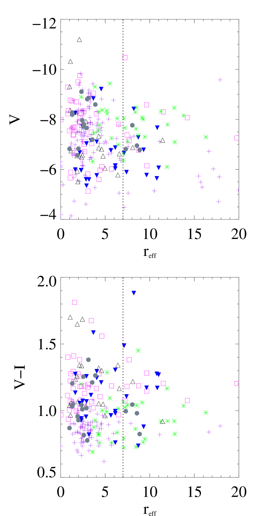
Figure 8 shows effective radii for ancient cluster candidates in all five galaxies as a function of luminosity and color. For comparison, we have added the half-mass radii of the Galactic GC system (Harris 1996). The dashed line marks an effective radius of 7 pc. In the Galaxy only $\sim 13$% of GCs are more extended than 7 pc. Our GC samples have extended cluster fractions range from 10% (M83) to 59% (M51). Formally, a Kolmogorov-Smirnoff (K-S) test finds that the size distributions in the Milky Way and M51 GC systems differ at a confidence level $>99$%. The results for the other cluster systems are less conclusive, but show a much higher probability (up to 85%) that they are drawn from the same parent distribution as the Milky Way GCs.

In the previous section, we reported the detection of a number of faint ancient cluster candidates in M101 and NGC 6946. These have a similar luminosity distribution to their faint counterparts in NGC 1023. However, the size distributions for the faint M101 and NGC 6946 clusters discovered in this work are similar to those of the more luminous GCs in their respective parent galaxies.

Could the observed difference of the M51 GC system simply be due to observational bias? The HST imaging is sufficient to select compact clusters in M51. In fact our catalog of young M51 clusters has a large fraction of compact objects (with $r_{eff}\sim 1.5-2$ pc). Finally, we note that the ancient cluster candidates in M51 are almost exclusively blue, while those in M81 are preferentially red. Although the physical reason for this difference isn’t clear, these results are broadly consistent with previous observations of a size-metallicity trend, since the M51 GCs appear significantly bluer (and more diffuse) than their redder, more compact M81 counterparts.

4.5. Numbers and Specific Frequencies of Globular Clusters in Spirals

4.5.1 Total Number of Globular Clusters

Our final globular cluster samples include 47, 21, 19, 29, and 34 objects for M81, M83, NGC 6946, M101, and M51 respectively. Given the very low fractional contamination estimated in $\S 3.5.1$, our survey provides unambiguous evidence that globular cluster systems exist in each of our target galaxies, despite the fact that M101, M83, and NGC 6946 are all of Hubble type Sc or later. In this section, we attempt to determine the total number of GCs associated with each host galaxy. We use the following basic recipe:

• We assume that the GC luminosity function turnover occurs at $M_{V}=-7.4$. The total number of GCs is defined as twice the number of GCs brighter than the turnover magnitude of the GCLF, where the GCLF is assumed to be a Gaussian (in magnitude units).

• The results of the artificial cluster experiments described in $\S 3.5.2$ are used to estimate the completeness of our GC samples. We determined an incompleteness fraction for each GC based on its V band luminosity. Each bin in the luminosity function was divided by the average completeness fraction of all objects in that bin to produce a completeness corrected value. Because we don’t track local background levels for the clusters, our completeness corrections are “averaged” over a range of environments, which we assume to be representative for the entire GC population.

• We then sum up the number of (completeness corrected) globular clusters to the expected turnover, and multiply this value by a factor of 2, to account for the faint half of the distribution.

• Finally, we correct for the (limited) spatial coverage of the galaxy in our survey. Our technique for estimating the correction or scale factor for the galaxies studied in this work is described below. Note however, that our technique to correct for this should not be considered a replacement for imaging data which has broader coverage.

For spirals, two techniques have generally been used to make a correction for limited galaxy coverage. Larsen et al.  (2001) constructed radial distribution functions of GCs. The caveat to this technique is that it requires a large population of GCs to avoid complications resulting from small number statistics. Kissler-Patig et al.  (1999) and Goudfrooij et al.  (2003) correct for spatial coverage by making a direct comparison with the GC locations in the Milky Way. This technique makes the implicit assumption that GC systems in external spirals have a similar spatial distribution as the GC system in our Galaxy. Goudfrooij et al.  (2003) find that the total number of GCs estimated for NGC 4594 using both methods described above gives consistent results. The estimated GC population in NGC 7814 is also similar between the two techniques (Goudfrooij et al. estimate $106\pm 28$ total GCs using the Galaxy-comparison technique, and Rhode & Zepf (2003) find $140-190$ GCs by fitting the radial profile of the GC system). Because we do not have sufficient numbers of clusters or radial coverage to use the former technique, we devised a procedure similar to the latter. We use data from the Milky Way GC system compiled in the McMaster catalog (Harris 1996), which contains 150 GCs. However, we adopt $N_{MW}=160\pm 20$ (van den Bergh 1999) as the total number of Galactic GCs. The undetected MW GCs are assumed to lie behind the Galactic bulge, and the locations of these “missing” clusters was synthesized by reflecting 10 known clusters within 2.0 kpc of the bulge in the projected “Y-Z” plane. In the following discussion of Galactic GC locations, X points toward the Galactic center, Y points in the direction of Galactic rotation, and Z toward the North Galactic Pole. There are essentially two different orientations which can be considered for external galaxies viewed face-on, corresponding to clusters with $+$ or $-$ Z locations (which side of the disk is observed). We created a mask defined by our spatial coverage of each galaxy, and then applied this mask to both face-on presentations of the Milky Way (i.e., the $\pm\mbox{Z}$ locations projected onto the X-Y plane of the Galactic disk). By calculating the fraction of the total GC system observable in each mask, we were able to determine a “scale factor” for the incomplete spatial coverage of our observations (taken to be the average from the two orientations): $S_{complete}=N_{MW}/N_{mask}$, where $N_{mask}$ is the number of GCs detected in the mask, and $N_{MW}$ is the total number of GCs in the Milky Way system. This technique makes the explicit assumption that GCs are found predominantly associated with bulges and/or halos of galaxies. If instead globular clusters in a given galaxy are associated with a thin disk, and can be seen above the dust layer from either side, then our technique will overestimate the number of clusters.

Our technique to derive the total number of GCs can be written as:

$$N_{GC}=2\times S_{complete}\sum_{i=V_{min}}^{V_{turnover}}\frac{1}{\langle f_{i}\rangle}~{}N_{V,i}$$ (1)

where $S_{complete}$ is the scale factor used to correct for the limited spatial coverage of the observations, the luminosity fuction is summed from the brightest magnitude bin $V_{min}$ to the magnitude bin covering the GCLF turnover; $\frac{1}{\langle f_{i}\rangle}$ represents the average fractional completeness for GCs in a given luminosity bin, and $N_{V,i}$ is the number of clusters observed in a given luminosity bin.

As discussed in $\S 4.1$, M101 and NGC 6946 do not appear to have a typical log normal GC luminosity distribution in magnitude space. The observations probe these galaxies deeply enough that we can push $\sim 1.5$ magnitudes beyond the expected turnover in the GC luminosity function. Having done this, we find an excess of faint, red, resolved clusters, a population which clearly does not exist in M81. Whether these objects are true ancient GCs formed early in the universe, or whether they have ages of a few billion years remains to be determined. For the purposes of discussing the total number of GCs in the three latest-type galaxies, we simply sum up the (completess corrected) clusters to the expected turnover ($-7.4$), and follow equation 1, thus explicitly excluding this “excess” faint population. In M101 and M83 if we sum up the (completeness corrected) GC sample to $M_{V}=-6$, the total number of clusters increases by a factor $\sim 1.8$. Because of M81’s proximity, we can reach almost the entire expected GC population. For this galaxy, we tried two approaches. First, we used the bright half of the GC luminosity function as representative of the faint portion, and second we summed the entire completeness corrected cluster population. Both techniques result in similar total GC populations for M81 (430 vs. 450), and we retain the numbers based on the second method.

Uncertainties in the total number of GCs are dominated by the correction for limited coverage. The distribution of Galactic GCs becomes stochastic as one moves away from the galaxy center, since they are not evenly projected in the X-Y plane at larger galactocentric distances. We attempted to place limits on the upper and lower fractional coverage by considering the full range of clusters covered if a given outer WFPC2 pointing was located at the same physical distance from the galaxy center, but at a different location. Additionally, uncertainties in the total number of clusters based on the unavailability of the $U$ filter for some fields were considered. The range in fractional coverage and likely contamination fraction were translated into uncertainties in the total number of GCs derived for each galaxy.

The calculated total GC numbers residing in each target galaxy and associated uncertainties are recorded in column 6 of Table 9. Previously, we estimated the M81 GC population to be $211\pm 29$ (Chandar, Tsvetanov, & Ford 2001). There were two weaknesses in our previous technique: 1) we didn’t explicitly make completeness corrections, and 2) our measurements hinged on fitting the radial profile of the GC system, which has very large uncertainties. The new results presented here supercede our previous numbers.

We make an independent consistency check on the number of GCs derived in M81 as follows. Using a single WFPC2 V band image, Davidge & Courteau (1999) estimated that $45\pm 12$ GCs brighter than $M_{V}=-7$ reside within the central 2 kpc of M81. Using our technique above, the MW GC system, when projected onto M81 (and accounting for distance, inclination and position angle), has $\sim 20$% of the visible population (on a given side of the disk) in the same area. This implies $48\pm 15$ GCs based on our estimated GC population, in good agreement with the Davidge & Courteau observations.

Table 9NUMBERS OF GCs AND SPECIFIC FREQUENCIES FOR SAMPLE GALAXIES

Galaxy	B/T	$M_{V}^{0}$	$M_{V}$	GC	GC	$S_{N}$	T
			bulge	(det)	(total)	total	total
M81	0.46	$-21.63$	$-20.60$	47	$450\pm 145$	$1.0\pm 0.3$	$1.9\pm 0.5$
M83	0.05	$-21.01$	$-18.51^{+0.75}_{-0.44}$	21	$150\pm 20\phantom{0}$	$0.6\pm 0.1$	$1.4\pm 0.2$
NGC 6946	0.02	$-21.46$	$-18.21_{-0.75}$	19	$90\pm 40$	$0.2\pm 0.1$	$0.7\pm 0.3$
M101	0.04	$-21.42$	$-18.17_{-0.75}$	29	$150\pm 40\phantom{0}$	$0.4\pm 0.1$	$1.2\pm 0.3$
M51	0.42	$-21.68$	$-20.73$	34	$220\pm 45\phantom{0}$	$0.5\pm 0.1$	$1.1\pm 0.2$

Note. — The derivation of the total number of clusters is given in $\S 4.5.1$, and explicitly excludes the faint, excess clusters in M101 and NGC 6946.

4.5.2 Bulge Luminosities

One of the goals of this work is to study the red metal-rich and blue metal-poor GC populations separately. In the Milky Way, there has been much recent evidence to support the view that inner, metal-rich GCs in spirals are associated with the Galactic bulge rather than the disk (Minniti 1995; Cote 1999). In order to test this concept, we need information on the relative contributions of the bulge and disk.

Because GC specific frequencies are traditionally normalized to the absolute V magnitude of the host galaxy, and by extension the estimated V magnitude for the bulge, it is preferable to use bulge/disk decompositions measured from a similar passband, such as found in Baggett, Baggett, & Anderson (1998). As a check on the Baggett et al.  (1998) results, we downloaded K band 2MASS images of our target galaxies and performed our own decompositions. It has been suggested that the near infrared is the ideal wavelength regime to study the stellar populations which make the dominant mass distribution in a galaxy (e.g., Rix & Rieke 1993). There are two main reasons for this. First, the extinction is lower by a factor of 10 between the B and K bandpasses, and second, the emission of old stellar populations peaks in the NIR. As bulge/disk decompositions are not the main goal of this work, we only briefly describe our techniques. We used the IRAF task ELLIPSE to create the surface brightness profiles, and then compared the results of fitting a double exponential vs. a de Vaucouleurs profile plus an exponential. These resulted in K band measurements of bulge and disk effective radii. To determine the K band surface brightness at these effective radii, we use the extended source 2MASS on-line catalog (http://pegasus.phast.umass.edu), where K band surface brightnesses at our best fit bulge and disk effective radii were read off from the available profiles. These values were then used to estimate the bulge-to-total (B/T) K-band luminosity ratios. If the Baggett et al. (1998) values differed significantly from our decompositions, we use the B/T values implied by our K-band fits to determine the bulge V band magnitude. In general, we find that M101, M83, and NGC 6946 (the three latest type galaxies) are best fit by a double exponential profile (although the double nucleus in M83 makes the results of our fit uncertain for this galaxy), and the results of our fits are adopted. The earlier type galaxies M51 and M81 are best fit by de Vaucouleurs bulge profile, plus an exponential disk, and we obtain results quite similar to those of Baggett et al.  (1998). Column 2 of Table 9 lists the adopted B/T values, column 3 gives the total V band galaxy luminosity, and column 4 gives the associated bulge luminosities.

4.5.3 Specific Frequencies

The total number of GCs can be normalized by galaxy luminosity or mass to facilitate comparison with other GC systems. The specific frequency, $S_{N}$ (as defined by Harris & van den Bergh 1981) $S_{N}\equiv N_{GC}\times 10^{+0.4(M_{V}+15)}$, is the number of GCs normalized by the total galaxy luminosity. Because different galaxy types are dominated by different stellar populations, normalizing by galaxy mass may give a more consistent comparison between galaxies with different star formation histories. Zepf & Ashman (1993) define $T\equiv\frac{N_{GC}}{M_{G}/10^{9}~{}M_{\odot}}$, where $M/L_{v}$ ratios of 6.1 (Sab-Sb), 5.0 (Sbc-Sc), and 4.0 (Scd-Sd) are used to convert galaxy luminosity to mass. The total T and $S_{N}$ values for our galaxy sample are presented in columns 7 and 8 of Table 9.

5. DISCUSSION

5.1. What is the nature of the faint clusters in late-type spirals?

As discussed in $\S 4.1$, NGC 6946 and M101 have formed a number of faint clusters which have integrated colors indistinguishable from globular clusters. Note however, that the U band photometric uncertainties are quite large for many of these. The presence of faint, ancient clusters has a significant influence on the observed luminosity distribution for our GC candidates; rather than turning over as expected, the clusters apparently follow a powerlaw distribution to the detection limit. Earlier, we found a similar situation in the late-type Local Group spiral M33 (Chandar, Bianchi, & Ford 2001). Qualitatively, the luminosity distribution of the faint GC candidates is similar to that found by Larsen & Brodie (2000) for faint, red, extended clusters in NGC 1023. Follow-up spectroscopy has established that the “faint fuzzies” in NGC 1023 rotate with the disk, unlike the more luminous, compact GCs, which have kinematics expected for halo/bulge objects. These faint diffuse clusters are ancient ($\geq 7$ Gyr), and relatively metal rich (Brodie & Larsen 2002). The faint M101 and NGC 6946 objects differ from “faint fuzzies” in that they are compact ($\S 4.4$), with sizes indistinguishable from the more luminous GC candidates in M101, and they are not preferentially red (metal-rich).

What is the nature of these faint clusters? Are they truly ancient, low mass clusters as suggested by their luminosities and colors? Because they are resolved, they cannot be individual stars, and their round morphology and location in the inner portions of the host galaxy (where almost no background galaxies are seen) is incompatible with a population of background galaxies. Are these analagous to the old open clusters in the Milky Way; ancient ($1-9$ Gyr), less massive (few $\times 10^{3}~{}M_{\odot}$) clusters residing in the (thin) Galactic disk? In Figure 9 we plot the color magnitude (upper panels) and color-color diagrams (lower panels) of old ($\geq 9.0$ log yrs) open Galactic clusters with available integrated photometry (Lata et al. 2002; Mermilliod & Paunzen 2003), and also include M101 and NGC 6946 clusters fainter than $M_{V}=-7$. For comparison, we also plot the Galactic GC population. Figure 9 illustrates two points. First, the old open clusters in the Galaxy appear fainter than the objects discovered in M101. However, current surveys of disk clusters are probably very incomplete due to large extinction in the disk. Thus it is likely that additional old open clusters exist, and these could overlap in luminosity with the objects presented here. The faint M101 clusters are defined so they lie in a luminosity range where Galactic GCs are falling off, and observational detection limits prevent us from observing old clusters as faint as known Galactic old open clusters. However, we cannot rule out that deeper photometry might reveal populations which overlap with old open cluster luminosities. The second point is that there is significant overlap in the colors of GCs and old open clusters (which are many Gyr younger). Partially, this is due to the age-metallicity degeneracy, since the somewhat more metal rich open clusters have slightly redder colors for their age than do the more metal-poor, older GCs. M101 cluster colors are consistent with formal age estimates $\mathrel{>\kern-10.00002pt\lower 3.87495pt\hbox{$\sim$}}3$ Gyr based on comparison with sub-solar BC00 models. Follow-up spectroscopy is needed to establish whether faint M101 and NGC 6946 clusters are younger than their more luminous counterparts and whether they reside in a disk.

While we cannot rule out that the faint M101/NGC 6946 clusters are counterparts to old Galactic disk clusters, a second possibility is that the faint red clusters are the low mass extension of the initial halo GC population, which were somehow able to survive internal and external dynamical evolution for a Hubble time. To explore this possibility, we compared available velocities for GCs in M33 fainter than $M_{V}=-7$, with their more luminous counterparts. Although there are only 17 such faint M33 GCs with available velocities, these have (halo) kinematics indistinguishable from more luminous M33 GCs (velocities taken from Chandar et al.  2002). Therefore in M33, regardless of the exact origin of ancient halo clusters, it appears that a larger fraction of lower massive clusters have been able to survive destruction over a Hubble time than found in the Milky Way or M31. The fact that these excess faint anceint clusters have only been seen in the latest-type spirals, where potentially the dynamical conditions are different from those in other well studied but earlier type galaxies, may provide clues to their survival.

5.2. Is There a Case for “Universal” halo globular cluster systems?

Goudfrooij et al.  (2003) studied edge-on spiral galaxies of different Hubble types. Based on their result that spirals with $B/T\mathrel{<\kern-10.00002pt\lower 3.87495pt\hbox{$\sim$}}0.3$ (i.e. Hubble type later than Sb) have very similar GC specific frequencies ($S_{N}=0.55\pm 0.25$), they suggest that this population represents a “universal”, old halo population which is present around each galaxy. Rhode & Zepf (2003) found a similar mass-normalized total number of metal-poor (presumably halo) GCs in the Sab spiral NGC 7814, as well as in the modest luminosity elliptical galaxy NGC 3379.

This is an important concept to test, considering the variety observed among the four most massive Local Group galaxies. While M33 has mostly halo GCs, in the LMC all ancient clusters reside in the (thin) disk (Freeman, Illingworth, & Oemler 1983). Thus, it is not clear whether all disk galaxies form halo systems of ancient clusters. In columns 7 and 8 of Table 9 we have compiled the estimated $S_{N}$ and T values for the galaxies presented in this work. We find that for all sample galaxies of type later than Sb (this only excludes M81, the earliest and most bulge dominated galaxy in our sample), the $S_{N}$ and T values are very similar, around 0.5 and $1.0-1.2$ respectively. Note that for M101 and NGC 6946, we have disregarded the population of faint, red clusters in deriving the estimated total numbers of GCs in these host galaxies. In M81, the observed $\sim 60$% blue fraction in our sample is similar to that found in the Milky Way and M31 GC systems. This results in $S_{N,blue}\sim 0.6$ and $T_{\mbox{blue}}\sim 1.1-1.2$, in the same range as we find for the later type spirals in our sample.

We conclude that all galaxies studied in this work, both early- and late- type, support the concept that (massive) spirals have formed a similar number of mass-normalized total GCs, with $S_{N}\sim 0.5$ and $\mbox{T}\sim 1.3\pm 0.2$. Since later-type galaxies are dominated in mass by their halos, this suggests that a “universal” population of halo GCs may have formed associated with all (massive) galaxies. This statement is predicated on the assumption that if the faint (low mass) clusters discovered in our Sc and later-type galaxies belong to the original halo GC population, their presence is the result of a difference in destruction timescales rather than formation mechanisms.

Table 10“SCORESHEET” FOR GLOBULAR CLUSTER SYSTEMS IN INDIVIDUAL SPIRAL GALAXIES

Galaxy	$M_{V}$	Type	$S_{N}$	T	$M_{V}$	$B/R$	univ	univ	disk	$r_{\mathrm{eff}}$
					peak	frac	halo?	bulge?	subpop		Refs
1. MW	$-21.3$	Sbc	0.6$\pm$0.1	1.3$\pm$0.4	$-7.4$	0.70	Y	Y	Y	Y	1
2. M31	$-21.8$	Sb	0.9$\pm$0.2	1.6$\pm$0.4	$-7.4$	0.66	Y	Y	Y	Y	2
3. M33	$-19.4$	Scd	0.6$\pm$0.1	1.6$\pm$0.3	$\mathrel{<\kern-7.00002pt\lower 2.71246pt\hbox{$\sim$}}\!-7.0$	$\cdots$	Y	$\cdots$	Y:	Y	3
4. NGC 55	$-19.5$	Sm	0.3$\pm$0.2:	1.6$\pm$0.3	$\cdots$	$\cdots$	$\cdots$	$\cdots$	$\cdots$	$\cdots$	4
5. NGC 253	$-20.2$	Sc	0.5$\pm$0.3:	1.1$\pm$0.5:	$\cdots$	$\cdots$	$\cdots$	$\cdots$	$\cdots$	$\cdots$	4,5
6. M81	$-21.63$	Sab	1.0$\pm$0.3	1.9$\pm$0.5	$-7.5$	0.6:	Y	Y:	Y	Y	6
7. NGC 6946	$-21.46$	Sc	0.2$\pm$0.1	0.7$\pm$0.3	$\mathrel{<\kern-7.00002pt\lower 2.71246pt\hbox{$\sim$}}\!-7.0$	$\cdots$	Y:	$\cdots$	$\cdots$	Y	6
8. M83	$-21.01$	Sc	0.6$\pm$0.1	1.4$\pm$0.2	$\sim\!-7.5$	$\cdots$	Y	$\cdots$	$\cdots$	Y	6
9. M101	$-21.42$	Scd	0.4$\pm$0.1	1.2$\pm$0.3	$\mathrel{<\kern-7.00002pt\lower 2.71246pt\hbox{$\sim$}}-\!6.0$	$\cdots$	Y	$\cdots$	$\cdots$	Y	6
10. M51	$-21.68$	Sbc	0.5$\pm$0.10	1.1$\pm$0.2	$<\!-8.0$	1.0	Y	N	$\cdots$	N	6
11. NGC 4594	$-22.20$	Sa	1.7$\pm$0.6	3.6$\pm$1.1	$\cdots$	$\cdots$	Y	Y	$\cdots$	$\cdots$	7
12. NGC 3628	$-21.03$	Sb	0.6$\pm$0.1	0.7$\pm$0.2		$\cdots$	Y	Y	$\cdots$	$\cdots$	7
13. NGC 4565	$-21.48$	Sb	0.6$\pm$0.2	1.0$\pm$0.3	$\cdots$	$\cdots$	Y	$\cdots$	$\cdots$	$\cdots$	7
14a. NGC 7814	$-20.46$	Sab	0.7$\pm$0.2	1.5$\pm$0.5	$\cdots$	$\cdots$	Y	N	$\cdots$	$\cdots$	7
14b. NGC 7814	$-20.46$	Sab	1.3$\pm$0.4	2.2$\pm$0.8	$\cdots$	$\cdots$	Y	Y:	$\cdots$	$\cdots$	5
15. NGC 4013	$-20.83$	Sb	1.1$\pm$0.3	2.2$\pm$0.7	$\cdots$	$\cdots$	Y	Y	$\cdots$	$\cdots$	7
16. NGC 4517	$-21.64$	Sc	0.6$\pm$0.2	1.4$\pm$0.5	$\cdots$	$\cdots$	Y	$\cdots$	$\cdots$		7
17. IC 5176	$-21.09$	Sbc	0.5$\pm$0.1	1.1$\pm$0.3	$\cdots$	$\cdots$	Y	N:	$\cdots$	$\cdots$	7

References. — (1) Ashman & Zepf 1998 (2) Battistini et al.  1993 (3) Chandar et al.  2001 (4) Beasley & Sharples 2000 (5) Rhode 2003 (6) this work (7) Goudfrooij et al.  2003

5.3. Is There a Case for “Universal” metal-rich bulge globular cluster systems?

In the Galaxy, the inner metal-rich GC subsystem has metallicity, kinematics, and spatial distributions comparable to those of the underlying bulge stars (e.g., Minniti 1995; Cote 1999). Forbes et al.  (2001) extended this evidence to suggest that the number of red, metal-rich GCs normalized by the bulge luminosity is constant in nearby spirals. They compared the GC systems of three spiral galaxies of different type (Milky Way=Sbc, M31=Sb, and M104=Sa), and argued that the bulge specific frequency, which they define as the number of metal-rich GCs within 2 bulge effective radii from the galaxy center divided by the total bulge luminosity, was consistent among these three galaxies, and similar to values found for field ellipticals. A similar pattern is seen in elliptical and lenticular galaxies, where the spatial distribution of metal-rich GCs (typically) closely follows that of the spheroidal light distribution, whereas the (blue) metal-poor GCS is usually more extended (e.g., Kundu & Whitmore 1998; Puzia et al.  1999; Barmby et al.  2002). If an association between the bulges of spirals and their metal-rich GC systems can be established, this would provide an important link between the formation of spheroidal systems in general and the formation of metal rich GCs.

An alternative scenario is the possibility that bulges form from the redistribution of angular momentum of inner disk stars via bar instabilities. In this “secular” evolution (e.g., Pfenniger & Norman 1990), galaxies can evolve along the Hubble sequence from late- to early- types. However, since only disk stars contribute to bulge formation in this model, GCs are not involved, and hence no (metal-rich) bulge GCs are expected.

In their study of 7 edge-on disk systems, Goudfrooij et al.  (2003) found evidence supporting an association of inner metal-rich GCs with spiral bulges. Their findings appear inconsistent with secular evolution. However, one bulge-dominated spiral galaxy, NGC 7814, did not show evidence for a system of inner, metal-rich GCs, implying that secular evolution is still a viable option for some systems.

In this section, we focus on the two earliest-type spirals in our sample, M81 and M51, where the number of GCs associated with bulge formation should be highest. In $\S 4.3$, we noted the apparent lack of metal-rich GCs in M51. Here, we quantify the expected number of metal-rich GCs associated with the M51 bulge, and compare with predictions based on the Forbes et al.  (2001) scenario. Figures 7a shows that there are four GCs in our M51 sample which appear to be metal-rich. Assuming that we are missing the faint portion of the GC luminosity function (correction factor $\sim 2$) and that there are a similar number of metal-rich GCs behind the disk, we estimate that M51 has no more than 16 metal-rich GCs associated with the bulge. Here we determine the number of metal-rich GCs predicted by the “universal” bulge system scenario. Assuming a bulge $S_{N}$ of 0.5 as given by Forbes et al.  (2001), and using the bulge $M_{V}$ value given in Table 9, 98 red GCs are predicted to reside within 2 bulge effective radii of M51. Because bulge luminosities can be difficult to estimate correctly from bulge/disk decompositions, we attempted to use other techniques to estimate the M51 bulge luminosity as well. The smallest estimate comes from the $\sigma-\mbox{black hole mass}$ relationship, and gives $M_{V}$ bulge $=-19.8$ (Wu & Han 2001). This bulge luminosity combined with the Forbes model ($S_{N}=0.5$) predicts 45 red GCs. This is still roughly a factor of $3$ larger than implied by our observations.

Therefore, we tentatively conclude that M51 does not follow the “universal” bulge GC population as suggested by Forbes et al. (2001). Because bar formation can be triggered via galaxy interactions, and M51 shows the clear signs of on-going interaction with its nearby barred companion NGC 5195 (one manifestation may be the many young stars and clusters seen in the central region; Lamers et al.  2002), we suggest that M51 is consistent with the idea of secular evolution resulting in bulge formation. An alternative explanation is that the $\sigma-\mbox{black hole mass}$ overestimates the total bulge luminosity by a factor of $\sim 3$ in M51.

Approximately 40% of our M81 GC sample appears to be metal-rich. Based on the total number of GCs estimated for M81, we calculate $S_{N}=1.0^{+0.4}_{-0.3}$ for the bulge normalized specific frequency, assuming the B/T ratio given in Table 9 and that 40% of the total M81 GC population is metal-rich. This range is similar to that found for the bulge dominated systems NGC 3628 and NGC 4594 (Goudfrooij et al.  2003).

Most of the red clusters discovered in this work are located beyond $2r_{eff}$ of the M81 bulge. In fact, red clusters in our sample are found in all studied WFPC2 fields, which cover a range of different environments. This is reminiscent of the metallicity/position distribution of M31 GCs. While we cannot directly comment on any bulge GC population in M81 due to our inadequate coverage of the most central portions, we note that Schroder et al.  (2002) found metal-rich GCs residing beyond two bulge $r_{eff}$ (based on spectroscopy). At face value, this suggests that M81 may also have retained a system of rotating disk GCs.

We conclude that our study finds mixed support for the concept that metal-rich GCs in spirals are associated with bulge formation. M51 in particular, which is similar in type to the Milky Way, appears to be lacking a metal-rich bulge GC population, and metal-rich GCs in general, despite some evidence that a central bulge does exist. This galaxy is consistent with a scenario of bulge formation through secular processes.

5.4. Implications for Galaxy Formation

Properties of GC systems in spiral galaxies are a promising tool for understanding the formation histories of disks, bulges, and halos. In this work, we presented the photometric properties for GC systems in five, nearby, low inclination spirals. Future follow-up spectroscopy for ages, abundances, and velocity information will provide additional constraints on GC system properties, and the formation of spirals. By way of summarizing what is currently known about spiral GC systems, we have compiled a “scoresheet” in Table 10. The following properties of GC systems are included in the indicated column: galaxy (1); total V band luminosity (2); galaxy type (3); specific frequency, $S_{N}$ (4); mass-normalized number of GCs, $T$ (5); magnitude of the GC luminosity function turnover (upper luminosity limits are given in some cases) (6); ratio of blue-to-red GCs (7); is the GC system consistent with a “universal” halo population? (8); did a constant (mass-normalized) number of metal-rich GCs appear to have formed in association with the bulge? (9); is there a disk population? (10); is the size distribution similar to that found in the Milky Way? (11); and finally the references (12).

Here, we use the entire sample presented in Table 10 to try and understand the formation of spiral GC systems in a broader context. As mentioned earlier, Goudfrooij et al.  (2003) suggest that all spirals, regardless of Hubble type, have formed a “universal” mass-normalized number of GCs in their halos. They suggest that a higher GC specific frequency should be observed in galaxies with dominant bulges, since a second, metal-rich population is expected to form associated with bulge stars. Rhode (2003) however, found evidence that the number of GCs depends primarily on the total luminosity (mass) of the host galaxy, and has little to do with Hubble type. Since their conclusion is based on a sample including four early-type galaxies and four spirals, it is not clear whether this is true for spirals in general. Below, we look for correlations between GC specific frequencies and host galaxy properties.

In Table 11 we compile mean and median values of $S_{N}$ and T for spiral GC systems by dividing the total sample into two groups: early vs. late-type, large vs. small bulge, bright vs. faint, and high vs. low mass. These show that in general, the T parameter, which was devised to roughly account for differences in the dominant stellar populations in galaxies of different types, shows more scatter than the specific frequency $S_{N}$. To further quantify any trends, in Figure 10 we show $S_{N}$ and T as a function of galaxy parameters (taken from Table 10). A linear fit was performed for each dataset, and is plotted if a correlation (at the $\mathrel{>\kern-10.00002pt\lower 3.87495pt\hbox{$\sim$}}2\sigma$ level) is found. The slopes from the fits are also recorded in Table 11. The strongest correlation $(4-5\sigma$) is between Hubble type and the $S_{N}$ of GC systems, in the sense that earlier-type spirals have larger numbers of luminosity normalized clusters. The second column of plots also show a correlation between $S_{N}$ and T with B/T ratio, although difficulties in bulge/disk decompositions may contribute to the somewhat weaker correlation ($\sim 3-4\sigma$) relative to that seen with Hubble type. The last two sets of panels show no evidence for a correlation of GC numbers with total luminosity or mass of the host galaxy.

Table 11MEAN SPECIFIC FREQUENCIES FOR GLOBULAR CLUSTER SYSTEMS IN SPIRALS

Group	range	$S_{N}$			T			N
		median	mean	slope	median	mean	slope
1. early-type	Sa-Sbc	0.90	0.90$\pm$0.11	$\cdots$	1.60	1.70$\pm$0.23	$\cdots$	12
2. late-type	Sc-Scd	0.60	0.54$\pm$0.10	$-$0.14$\pm$0.03	1.40	1.32$\pm$0.18	$-$0.18$\pm$0.08	7
3. large bulge	$B/T>0.2$	0.90	0.92$\pm$0.13	$\cdots$	1.60	1.72$\pm$0.27	$\cdots$	10
4. small bulge	$B/T\leq 0.2$	0.60	0.60$\pm$0.08	0.80$\pm$0.23	1.40	1.42$\pm$0.15	1.10$\pm$0.49	9
5. high mass	log($M/M_{\odot})$ $>11.1$	0.60	0.72$\pm$0.12	$\cdots$	1.30	1.52$\pm$0.25	$\cdots$	11
6. low mass	log($M/M_{\odot})$ $\leq 11.1$	0.70	0.83$\pm$0.12	0.25$\pm$0.30	1.60	1.66$\pm$0.17	0.38$\pm$0.57	8
7. bright	$M_{V}\leq-21.25$	0.60	0.72$\pm$0.15	$\cdots$	1.30	1.53$\pm$0.28	$\cdots$	9
8. faint	$M_{V}>-21.25$	0.70	0.81$\pm$0.10	$-$0.12$\pm$0.25	1.60	1.62$\pm$0.18	$-$0.05$\pm$0.13	10

Note. — Uncertainties in the mean are calculated as $\sigma/\sqrt{N}$

6. SUMMARY AND CONCLUSIONS

We have studied the properties of GC systems in five nearby, low inclination spirals using multifilter HST WFPC2 imaging. By using morphological information, we are able to separate clusters from individual stars, background galaxies, and blends. Crude spectral energy distributions from broadband filters or color information are used to distinguish between young and ancient clusters, and we detect GC systems in all five target galaxies. We find that the U band is crucial to separate reddened young clusters from ancient clusters. Below, we summarize the main conclusions from our study.

1. Based on estimated intrinsic colors, the M81 GC system has an extended metallicity distribution. This argues for the presence of both metal-rich and metal-poor GCs. This extended nature was not obvious in a previous study, when only single (BVI) colors were tested. However, by combining two color measurements together and including the U band, we find evidence that the color distributions are similar to those in the Andromeda and Milky Way GC systems. The M101 GC sample also has an extended color distribution. By contrast, our M51 cluster sample has a narrower and bluer color distribution, similar to that of blue, metal-poor Galactic globulars. We suggest that the lack of inner, red GCs in M51 is consistent with a secular origin for the M51 bulge.

2. The GC luminosity distributions for M101 and possibly NGC 6946, two of three later-type galaxies, appear to continue increasing to magnitudes fainter than $M_{V}\sim-7.4$, the expected turnover in the GC luminosity function. This is similar to what we found earlier in M33, another late-type spiral. In general, the colors of these excess, faint clusters do not differ significantly from those of old, open clusters in the Galaxy, or from more luminous GCs in the same galaxies. We suggest that faint GC candidates in later-type spirals may be either intermediate age ($3-9$ Gyr) disk clusters, or possibly the low mass extension of the original GC population, which survived destruction due to different dynamical conditions in later-type spirals when compared with earlier type galaxies.

3. We made a comparison of the effective radii distributions for GCs in our five target galaxies. All but M51 have distributions which are similar to that in the Milky Way. GCs in M51 however, are more extended on average, and $\sim 1/2$ our sample has sizes consistent with the “faint fuzzies” discovered in NGC 1023, although the colors and luminosities are quite different.

4. We find that the total GC populations in later-type spirals, and the blue subsystems in earlier-types are consistent with forming a “universal” halo population, as suggested by Goudfrooij et al. (2003), with T$=1.3\pm 0.2$ and $S_{N}=0.5\pm 0.2$.

5. Finally, by combining our sample with specific frequency values for other nearby spirals taken from the literature, we find that overall T and $S_{N}$ increase with morphology, from late- to early-type spirals (if faint excess clusters in later-type spirals are excluded from the calculation). This is consistent with a scenario where all massive spiral galaxies form a relatively constant number of halo GCs, and earlier types formed an additional, metal-rich bulge and/or disk population. We find no tendency for more luminous or massive spirals to have larger normalized GC populations than their less luminous/massive counterparts.

Figure 1.— The HST WFPC2 field pointings used in this study are overlaid on Digitized Sky Survey images of each target galaxy (M81, M83, NGC 6946, M101, and M51). A scale of five arcminutes is shown in each figure, and WFPC2 footprints shown in blue include U band imaging.

Figure 2.— The reddening $E_{B-V}$ distribution functions are shown for our “all cluster” catalogs in M101 and M51. These were derived using the simultaneous age/$E_{B-V}$ fitting technique described in $\S 3.3.1$.

Figure 3.— Average V band completeness curves as determined from artificial cluster experiments are shown for each target galaxy.

Figure 4.— The color-luminosity distributions of GCs presented in this work are shown. The luminosity has been corrected for distance and foreground extinction, and the colors have been dereddened by the foreground value only. The dotted lines show typical $(V-I)_{0}$ colors for blue and red GC subpopulations in ellipticals and lenticulars.

  

  

  

Figure 5.— Globular cluster luminosity functions for each galaxy are plotted. These have not been corrected for incompleteness. The dotted line represents that average 80% completeness level for each cluster sample. For comparison, we have added the luminosity function for M33 GCs (Chandar et al.  2001) in the last panel.

Figure 6.— Top Panels: The $(V-I)$ vs. $(U-B)$ color-color diagram is shown. The lines are solar (solid), 1/5 solar (dotted), and 1/50 solar (dashed) BC00 metallicity models. The direction of the reddening vector is shown by the arrows. Milky Way and M31 GC colors have been dereddened (both foreground and internal). The GC colors from this work have been dereddened by only the foreground values. The solid lines show the best fit to dereddened M31 GCs from the Barmby et al.  (2000) catalog (left), and the best fit to the M81 plus M51 data points (right). Bottom Panels: The distribution of two color values (see text for description) are plotted. These show the extended nature of the M31 and Milky Way GC systems, as well as those in M81 and M101.

Figure 7.— Top Panels: The $(V-I)$ vs. $(B-V)$ (left) and $(V-I)$ vs. $(U-V)$ (right) color-color diagrams are shown. BC00 models and GCs are as in Figure 6. Bottom Panels: The distribution of cluster positions in color-color space along the M31 GC locus are shown. Derivation of these values are described in $\S 4.2$.

Figure 8.— Measured effective radii for our GCs. Purple crosses are the half-mass radii of the Galactic system. The dashed line at 7 pc is that used by Larsen & Brodie (2000) to separate “faint fuzzies” from more compact clusters in NGC 1023.

Figure 9.— The upper panels shows color-magnitude diagrams for “faint” M101 (blue triangles) and NGC 6946 (gray filled circles) globular cluster candidates (defined as $M_{V}\geq-7$). These are compared with the absolute luminosities and dereddened colors of Galactic globular clusters (crosses) and old ($>9.0$ log yrs) open clusters (red open circles). The lower panels shows color-color distributions for all four cluster populations.

Figure 10.— Figures showing spiral GC systems’ specific frequencies and T values as a function of Hubble type, bulge/total, total V luminosity of the galaxy, and galaxy mass.