Design and imaging performance of achromatic diffractive/refractive X-ray and Gamma-ray Fresnel lenses

Abstract

Achromatic combinations of a diffractive Phase Fresnel Lens and a refractive correcting element have been proposed for X-ray and gamma-ray astronomy and for microlithography, but considerations of absorption often dictate that the refractive component be given a stepped profile, resulting in a double Fresnel lens. The imaging performance of corrected Fresnel lenses, with and without ‘stepping’ is investigated and the trade-off between resolution and useful bandwidth in different circumstances is discussed. Provided the focal ratio is large, correction lenses made of low atomic number materials can be used with X-rays in the range approximately 10–100 keV without stepping. The use of stepping extends the possibility of correction to higher aperture systems, to energies as low as a few kilo electron volts and to gamma-rays of $\sim$ mega electron volt energy.

1 Introduction

Zone plates and Fresnel lenses are widely used at X-ray wavelengths for microscopy and microlithography (e.g. references eg1 ; eg2 ; eg3 ) and have been proposed for use in X-ray and gamma-ray astronomy paper1 ; paper2 ; gorenstein2003 ; gorenstein2004 . We here concentrate on phase Fresnel lenses (PFLs) using the terminology of Miyamoto miyamoto . In PFLs the optical thickness profile is such that the phase shift is everywhere exactly the same, modulo $2\pi$, as that of an ideal refractive lens. This leads to a structure with the same periodicity as a zone plate but with much higher efficiency.

PFLs are attractive for high energy astronomy, for which they offer the prospect of extremely high angular resolution. Performance can be diffraction limited, even in the gamma-ray part of the spectrum. For diameters of a few metres this limit corresponds to $\sim$ 0.1–1 micro arc second ($\mu^{\prime\prime}$), opening up the possibility of imaging the black holes in distant galaxies, for example. Equally important is the ability of PFLs to concentrate flux from a large collecting area onto a small, low-background, detector, resulting in orders of magnitude improvement in sensitivity compared with current techniques.

In microlithography and microscopy, PFLs and zone plates can provide spatial resolution somewhat finer than the finest scale of the structure of the lens, which can beeg2 of the order of a few tens of nm.

PFLs suffer from two major disadvantages. First, the focal lengths tend to be long – values of as much as several million kilometers have been discussed for astronomy paper1 . Second, in common with other diffractive optics, they are highly chromatic. For PFLs, as for simple zone plates, the focal length is inversely proportional to wavelength, so the good imaging performance is only available over a narrow spectral band.

Surprisingly, with the developments of techniques for formation flying of two spacecraft the first problem – that of focal length – does not seem to be unsurmountable imdc-study-report . Furthermore accepting and using very long focal lengths ameliorates chromatic effects spie2003 . There are, though, practical limits to how far one can go in this direction. For example the distance between spacecraft flying in formation and carrying the lens and detector of an astronomical telescope is limited by the thrust and fuel consumption of the thrusters that are necessary to overcome gravity gradient effects and also by the size of the detector necessary for a given field of view.

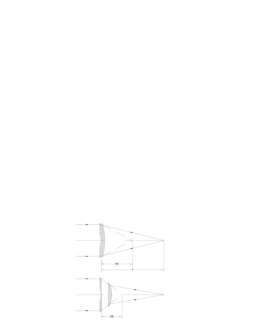
Figure 1: Use of a refractive lens to compensate for the chromatic effects in a PFL. Upper : first order correction. Lower : second order correction.

In some circumstances another consideration that can help overcome the limitations associated with chromaticity is that a PFL can be used at wavelengths over a wide band if the detector distance is adjusted for each wavelength in turn. There is little loss in image quality or efficiency paper1 , but of course the observing time for any one wavelength is only a fraction of the total time available.

It has long been known faklis-morris that full achromatic correction of the dispersion of a diffractive component is possible using another diffractive component in the configuration originally proposed by Schupmann schupmann . However this arrangement is unlikely to be useful in the X/gamma-ray case because it requires a further optical component to image the aperture of one diffractive component onto the other. This additional optical component can be smaller, but it has itself to be achromatic. Bennett bennett76 has discussed the fact that there are intrinsic limits on correction of diffractive elements by other diffractive elements.

Figure 2: The thickness, $t_{2\pi}$, necessary to produce a phase shift of 2$\pi$ for different materials (P-C indicates Polycarbonate).

Of interest here us the possibility, pointed out in a number of papers paper2 ; wang ; gorenstein2004 of making an achromatic X-ray or gamma-ray system by combining a diffractive component with a refractive one. The advantages and limitations of these schemes are examined here. Emphasis is placed on astronomical telescope designs, but reference is also made to laboratory applications.

Figure 3: The absorption length divided by $t_{2\pi}$ for the materials in Fig. 2.

2 Diffractive/refractive achromatic designs

At x-ray and gamma-ray wavelengths the real part of the refractive index of a material is usually written $\mu=1-\delta$, where $\delta$ is small and positive ($10^{-3}$–$10^{-10}$), corresponding to refractive indices slightly less than unity. At high energies note and away from absorption edges, $\delta$ is approximately proportional to $\lambda^{2}$, leading to a variation of the focal length of a refractive lens $D=(\lambda/f_{r})(df_{r}/d\lambda)\sim-2$. Wang et al.wang have suggested the use of the very much larger anomalous dispersion in the region of the K and L absorption edges, but this occurs only in very narrow bands. We here concentrate here on what can be achieved with $D\sim-2$.

For a diffractive lens $D=-1$, so it follows paper2 that one can form an achromatic pair with combined focal length $f$ can by placing a diffractive component in contact with a refractive one (Fig. 1a). If, as in Fig. 1b, the two components are separated gorenstein2004 by a distance $S$, then $d^{2}f/d\lambda^{2}$ can be made zero as well as $df/d\lambda$  ($f$ is the focal length of the combination measured from one of the components; here we use the first). However we shall see in section 3 that some degree of transverse chromatic aberration is inevitable if the separation is non-zero.

The problem with either of these forms of refractive correction is that in most practical circumstances the refractive lens must be very thick. Suppose that the diffractive component is operating in order $N_{d}$ (so that for a PFL the steps correspond to a phase shift $N_{d}2\pi$; usually $N_{d}=1$) and that it has $N_{z}$ annuli (or zone pairs for a zone plate). It will introduce a differential phase shift $N_{z}N_{d}2\pi$ between the centre and the periphery. In both the contact and separated pair cases, the refractive component must counteract half of this difference. Thus it must have a central thickness $t_{2\pi}N_{z}N_{d}/2$, where $t_{2\pi}$is the thickness which introduces a phase shift of $2\pi$.

This thickness should be compared with the attenuation length, $\>\Lambda$, of the material. Note that the relevant value of $\Lambda$ is one which includes the effects of losses by incoherent (Compton) scattering as well as by photoelectric absorption and, for high energies, pair production. Fig. 2 shows $t_{2\pi}$ for various materials and in Fig. 3 the ratio $Q=\Lambda/t_{2\pi}$ is plotted. If $N_{d}N_{z}\stackrel{{\scriptstyle>}}{{\sim}}Q$ then correction by a simple refractive lens as in Fig. 1 would require a lens in which the absorption losses at the centre would be large. Consequently there is a practical limit on the size of a diffractive lens that can be corrected by a simple refractive element; its diameter, $d$, must be less than about $k(f_{0}\lambda_{0}Q)^{1/2}$. Here $k$ is $2\surd 2$ for the contact pair case and $4/\surd 3$ for a separated pair and the subscript zero refers to values at the nominal design energy. It can be shown that the limit used here corresponds to requiring a mean transmission of $1-e^{-1}$, or 61%.

$Q$ is effectively the largest number of zone (pairs) in a diffractive lens which can be corrected in this way (assuming $N_{d}=1$). As shown in Fig. 3, $Q$ can reach a few hundred, the highest values being attained with materials of low atomic number ($Z$) and with photons of energy approximately $10-100$ keV. Within this energy band, and provided that a large focal ratio $f/d$ requiring a limited number of zones is acceptable, the simple configurations shown in Fig. 1 can be used. The design and performance of such systems are discussed in the Subsection 4A.

Where the absorption of a simple refractive corrector would be prohibitive, the natural solution is to reduce the thickness in steps. The performance of such configurations is examined in Subsections 4B and 4C.

3 Design parameters

For an achromatic contact doublet with net focal length $f$ which combines a diffractive component, for which $D=-1$, with a refractive one having $D=-2$, the focal lengths of the two components need to be $f_{d}=f/2$ and $f_{r}=-f$ respectively.

If the two lens components are not in contact but separated by distance $S$, the transfer matrix between the input aperture and a detector plane distance, $f_{0}$ beyond it, is

$$\left(\begin{array}[]{cc}A&B\\ C&D\end{array}\right),$$ (3)

where, assuming $D=-2$,

$$\left.{\begin{array}[]{ccl}A&=&1-{\displaystyle{{{\mathcal{E}f_{0}f_{1}+\mathcal{E}^{2}f_{0}f_{2}-f_{0}S-\mathcal{E}f_{1}S+S^{2}}\over{\mathcal{E}^{3}f_{1}f_{2}}}}}\\ B&=&f_{0}-S\ {\displaystyle{\frac{f_{0}-S}{\mathcal{E}^{2}f_{2}}}}\\ C&=&{\displaystyle{-\>{{\mathcal{E}f_{1}+\mathcal{E}^{2}f_{2}-S}\over{\mathcal{E}^{3}f_{1}f_{2}}}}}\\ D&=&1-{\displaystyle{{S\over{\mathcal{E}^{2}f_{2}}}}}\end{array}}\right\},$$ (4)

and where $\mathcal{E}$ is the photon energy normalised such that $\mathcal{E}=1$ for $\lambda=\lambda_{0}$. For parallel incident radiation to be focussed at $f_{0}$, we set the term $A$ to zero. Requiring that $df/d\mathcal{E}=d^{2}f/d\mathcal{E}^{2}=0$, as discussed above, leads to the configuration shown in Fig. 1b in which

$$\left.{\begin{array}[]{rcl}S&=&f_{0}/9\\ f_{d}&=&f_{0}/3\\ f_{r}&=&-(8/27)\,f_{0}\end{array}}\right\}.$$ (5)

However the term $B$, which dictates the plate scale, is then $f_{0}(1+1/(3\mathcal{E}^{2}))$. The energy dependence of $B$ implies that there is transverse chromatic aberration (lateral colour). If one places the alternative constraints $A=df_{0}/d\mathcal{E}=dB/d\mathcal{E}=0$, the contact pair ($S=0$) case discussed above is the only solution.

The transverse chromatic aberration is not necessarily an over-riding problem. It has little impact if the lens is used primarily as a flux collector – one of the important potential astronomical applications. Moreover, in imaging applications in which the detector has the capability of determining the energy of each photon with adequate resolution, the effect can be corrected during data analysis. However, it may limit the usefulness of this configuration in some applications, for example, in microlithography.

Table 1: Example of a lens using unstepped refractive correcting elements for an astronomical application. Nominal energy 78.4 keV; focal length $1\times 10^{8}$m.

Configuration	Singlet	Contact	Separated
Diffractive component:-
Diameter (mm)	1310	1310	1070
Focal length (m)	$10\times 10^{7}$	$5\times 10^{7}$	$3.33\times 10^{7}$
Pitch (min) ($\mu$m)	2420	1210	985
Separation (m)		0	$1.11\times 10^{7}$
Refractive component:-
Diameter (mm)		1310	715
Focal length (m)		$-10.0\times 10^{7}$	$-2.96\times 10^{7}$
Thickness (mm)		39	39
Bandpass (keV)	0.1	4.7	27.7

The refractive component is assumed to be made of beryllium. The diameters of the achromatic combinations are chosen according to the guidelines in the text, and so the theoretical efficiency is 61% in each case. The singlet is assumed to have the same diameter as the contact pair, though absorption does not preclude it being made larger. The bandpass quoted is full width at half maximum of the on-axis response.

Table 2: Example of a lens using unstepped refractive correcting elements corresponding to that in Table 1 but for a laboratory application. Nominal energy 10 keV; focal length 1 m. Other details as Table 1.

Configuration	Singlet	Contact	Separated
Diffractive component:-
Diameter (mm)	0.511	0.511	0.417
Focal length	1.0	0.500	0.333
Pitch (min) ($\mu$m)	0.486	0.243	0.198
Separation (m)		0	0.111
Refractive component:-
Diameter (mm)		0.511	0.278
Focal length (m)		$-1.0$	$-0.296$
Thickness (mm)		9.57	9.57
Bandpass (keV)	0.03	0.8	2.9

4 Imaging performance

Figure 4: The on-axis response of lenses for a nominal design energy of 78.4 keV and with the parameters given in Table 1. The dotted lines show the response in the absence of absorption. Curves are normalised so the the peaks values are proportional to the effective areas. The peak response of the separated pair is lower than that of the contact pair because the absorption considerations discussed in section 2 require a smaller diameter. Variations in image brightness linked to changes of the diffraction limited resolution with energy have been removed.
File: skinner-achrom-fig4.eps

The complex amplitude of the response at distance $f_{0}$ and radial offset $y$ to parallel radiation falling at normal incidence on a thin lens of arbitrary circularly symmetric profile, is

$$\int_{0}^{r^{2}}J_{0}\left({{y\surd s}\over{\lambda f_{0}}}\right)exp\left[-{t(s)\over{\Lambda}}+i\pi\left({t(s)\over{t_{2\pi}(\lambda)}}-{{s+y^{2}}\over{f_{0}\lambda}}\right)\right]ds.$$

Here the total thickness $t(s)$ of the lens combination, is specified in terms of the parameter $s=r^{2}$ rather than radius $r$. Assuming the wavelength dependence of $t_{2\pi}$  corresponding to $D=-2$, rewriting in terms of energy, $\mathcal{E}$, and allowing for the possibility that the incoming radiation is not parallel, so that the phase $\phi$ will be a function of $s$, yields for the term in square brackets

$$\left[-{t(s)\over{\Lambda}}+i\pi\left({t(s)\over{t_{2\pi}(\lambda_{0})}}{1\over{\mathcal{E}}}-{{s+y^{2}}\over{f_{0}\lambda_{0}}}{\mathcal{E}}+\phi(s)\right)\right].$$ (6)

Numerical integration of this function provides simple and precise evaluation of the response of a contact pair and, applied twice, the response of a separated pair to on-axis radiation.

4.1 Unstepped correctors

To illustrate the advantages gained with a simple unstepped correction lens, either in a contact pair and as part of a separated pair, Table 1 presents some example values for a space instrument having a very long focal length ($10^{5}$ km) and working at the astronomically interesting energy of 78.4 kev (⁴⁴Ti decay). Fig. 4 shows the on-axis response as a function of energy. The 0.1 keV bandpass of the uncorrected lens can be increased to 4.7 keV (contact pair) or 27.7 keV (separated pair). The bandwidth of the separated pair is sufficiently large that a single configuration could observe simultaneously at the energy of the 78.4 keV ⁴⁴Ti line and at that of the 67.9 keV line which accompanies it, as well as covering a large swath of continuum emission.

The on-axis point source response function is very close to the Airy function of an ideal lens, but is modified slightly by the apodizing effect of the radially varying transmission. The width of the point source response function is reduced by a few percent and the intensity of the first sidelobe is increased by $\sim$50%.

The contact pair has extremely low geometrical aberrations over a very wide field of view, as would be expected for a thin lens with a very large focal ratio. For a separated pair, the field of view is limited by vignetting at the corrector and this diameter has to be made somewhat larger than the minimum 2/3 $d_{d}$ needed for on-axis radiation, with a consequent increase thickness (and hence absorption). Within the vignetting-limited field of view geometrical abberations are entirely negligible.

It is natural to ask whether the configurations considered here for space astronomy could be scaled to be useful for laboratory applications. Table 1 show parameters for a 1 m focal length system working at 10 keV. Concentrating on the separated pair, the thickness/diameter ratio of the corrector lens would be 9.57 mm/0.278 mm = $\sim$34 in place of 39 mm/715 mm = 0.055. Mechanically this is very far from a ‘thin lens’ ! Because the radiation is always nearly paraxial, optically the thin lens approximation used in the above analysis remains a good first approximation, though no more than that. A small fourth order term in the profile, amounting to 0.1% of the thickness, is sufficient to correct the on-axis response. Off-axis aberrations then remain smaller than the diffraction-blurring over a field 1.6 mm in diameter containing $>10^{7}$ resolvable pixels. (In order to preserve the analogy with the astronomical case, focussing of a parallel input beam is assumed here. The 50% encircled power diameter is used as a measure of resolution and it has been assumed that the corrector is oversized by 10% to reduce vignetting.)

The examples quoted here represent approximately the extremes of size and of high and low energy for which unstepped configurations are likely to be attractive.

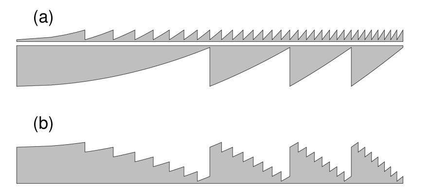
Figure 5: Profile of diffractive lens and stepped compensating refractive component. The example shown corresponds to $N_{d}=1,\>N_{r}=4$. (a) Two distinct components in contact. (b) A single component with the same thickness profile.

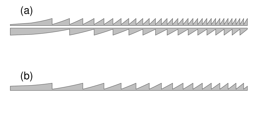
Figure 6: Same as Fig. 5, but for $N_{d}=1,\>N_{r}=1$. The combined profile (b) is identical to that of a simple PFL, so clearly in this limit no compensation is achieved.
File: skinner-achrom-fig6.eps

4.2 Stepped contact pair

As has been suggested above, the natural solution to excessive absorption in the refractive component is to reduce the thickness of the refractive component in a stepwise fashion (Fig. 5). Ideally the steps would be an integer number, $N_{r}$, times $t_{2\pi}$ but this cannot be exactly true for all energies. We consider first contact pairs.

There are limits to the stepping process as can be seen by noting that in the case of a contact pair in which the two components are made from the same material, all that is really important is the total thickness, $t(s)$. With $N_{r}=N_{d}=1$ the resulting thickness profile of a contact pair would be as shown in Fig. 6, which is that of a simple (chromatic) PFL of focal length $f$. At the opposite extreme, for $N_{r}>N_{z}N_{d}/2$, no steps occur.

We will here consider the performance of a thin contact achromatic pair (Fig. 1a) with intermediate degrees of ‘stepping’, $N_{d}<N_{r}<N_{z}N_{d}/2$.

To illustrate this case we take the case of a lens for imaging 500 keV gamma-rays having a diameter of 2.048 m (511 keV or the energies of other lines of astrophysical interest could equally have been chosen). Figure 3 shows that at this energy $Q$ is about 38 for any material of which the atomic number is not too high. This independence of material arises when the dominant loss mechanism is Compton scattering – $\Lambda$ then depends simply on the density of electrons, as does $\delta$. Thus although the lens is here assumed to be made from polycarbonate, similar performance could be obtained from many other materials. According to the criterion of section 2 the maximum diameter for a simple unstepped corrector would be 0.78 m for a focal length of $8\times 10^{8}$ m.

Figure 7: The on-axis response of achromatic contact pairs with different degrees of stepping of the refractive component, characterised by $N_{r}$, where the thickness is reduced modulo $N_{r}t_{2\pi}$. The focal length and diameter are kept constant. See Table 2 for detailed parameter values. The dashed lines show the response if there were no absorption. It can be seen that large values of $N_{r}$ give a response which is more nearly continuous as a function of energy but with absorption losses which become more and more serious. The energies indicated by B,C,D,E are those for which the point source response functions are shown in Fig. 10.

To illustrate the effect of different design options we consider variations on a ‘reference’ design with $N_{r}=64$ and a focal length of $8\times 10^{8}$ m. The assumed parameters are given in Table 4.

The calculated on-axis response for different values of $N_{r}$, either side of the reference design value, is shown in Fig. 7 and the effect of different focal lengths in Fig. 8. A series of peaks occurs within an envelope which is dictated by the uncorrected higher order terms in the Taylor expansion of $f$. The total response, integrated over all the peaks is shown in Fig. 9. As would be expected, for large $N_{r}$ the absorption negates the gain from having more peaks, the optimum in the example case being at $N_{r}\sim 50$ according to this criterion.

The spacing of the peaks is $E_{0}/N_{r}$, where $E_{0}$ is the nominal design energy. Their fractional width is inversely proportional to $N_{z}$, the number of annuli in the refractive component, just as the finesse of a Fabry-Perot interferometer depends on the number of interfering beams. Thus if $N_{r}$ (and hence the thickness and the absorption loss) is kept constant, long focal lengths widen the peaks and increase the integrated response.

The point source response function at energies between the peaks of the on-axis response is obviously an important consideration. For energies away from these peaks the flux is spread into an extended diffraction pattern with concentric rings having a characteristic width which is comparable in scale with the width of the ideal PSF (Fig. 10).

For practical applications in which an image is to be acquired, one can consider two possible situations. If one has an energy-resolving detector capable of recording separate images for each of the energies at which the image response differs significantly, then post processing can recover most of the imaging performance of an ideal lens. If however the energy resolution of the detector is insufficient to isolate the peaks in the on-axis response, then the effective angular resolution will be degraded by mixing of the different responses. The point source response function will then be one which is averaged over all energies within the band, as shown by the continuous curves in Fig. 10. In the example used here, the half power diameter would be degraded from 0.27$\mu^{\prime\prime}$(about 1 mm) to 1.8$\mu^{\prime\prime}$.

Table 3: Width of point source response function of the lenses considered in Table 4 and in Fig. 7

	Full Width	Half Power
Optical system	Half Maximum	diameter
and energy	(micro arc secs)	(micro arc secs)
Ideal diffraction-
limited lens	0.265	0.270
Achromat with
absorption (500 keV)	0.260	0.275
Ditto (averaged
response 450–550 keV)	0.265	1.80

Table 4: Parameters for the example gamma-ray lenses for astronomical applications for which the performance is shown in Fig. 7–9. Parameters in common are:- nominal energy: 500 keV, diameter: 2048 mm, material: polycarbonate. The ‘reference’ design values are in boldface.

Figs.	Focal	Diffractor	Refractor
	length, $f_{0}$	Zones	Step	Zones	Thickness
	(m)	$N_{z}$	$N_{r}$	$N_{zr}$	(mm)
			256	1	605
			128	2	302
			64	4	151
7,9	$8\times 10^{8}$	512	32	8	75
			16	16	38
			8	32	19
			(none)		2.4
	$2\times 10^{8}$	2048
	$4\times 10^{8}$	1024
8	$\bf{8\times 10^{8}}$	512	64	4	151
	$1.6\times 10^{9}$	256
	$3.2\times 10^{9}$	128

If the compound lens is to be used to increase the bandpass of a projected image, in microlithography for example, a degradation of resolution like that in Fig. 10 will usually have to be accepted. It is possible that the multiple peaks in the response might be adjusted to correspond to multiple lines in a fluorescent X-ray source or in synchrotron radiation from an undulator, or to multiple astrophysical lines such as the 57.9/78.3 keV Ti line pair discussed in section 4A.

Where the compound lens is used as a flux concentrator, a small detector will receive the multi-peaked response seen in Fig. 7, while for a larger one the troughs will be filled in.

Figure 8: As Fig. 7 but showing the effect of differing focal lengths for a particular value of $N_{r}$ (=64). Shorter focal lengths require a more powerful correction lens which, for a given $N_{r}$, is divided into a larger number of zones, resulting in narrower individual peaks in the energy response. In the case of the central plot showing the reference design, which would otherwise be a repeat of the corresponding plot in Fig. 7, the dashed line indicates how the response differs when seen by a detector integrating over a 5 mm radius.

Figure 9: The total on-axis response to a point source, integrated over energy, for the lens in Fig. 7 and the corresponding peak response, shown for different degrees of stepping. The dashed lines again show the results in the absence of absorption. Points for the separated pair described in section 4.3 are also shown.

4.3 Stepped separated pair

Stepping can, of course, be used with a separated achromatic pair. We content ourselves here with presenting (Fig. 11) the on-axis response of a separated lens pair version of the reference gamma-ray lens design considered in section 4.2.

As for a contact pair, the response as a function of energy has multiple peaks whose number and width are a function of the degree of stepping. Again between these peaks the flux is spread over a larger region, so the PSF is again broadened unless photons with these intermediate energies can be ignored. The detailed processes which give rise to the peaks and troughs are different because there is no longer a one-to-one correspondence between regions of the two optical elements. Although in the region of ${E}_{0}$ the spacing of the peaks is the same as for the contact pair, the spacing is not constant but varies as $E^{2}$. Their width is typically a factor of $\sim 1.5$ smaller than for the reference contact pair case, which has the same $N_{r}$ and the same absorption losses. In consequence the gain in integrated response is only a factor of 1.65.

Figure 10: (a) Point source response function of the lens in Fig. 7, averaged over energies 450-550 keV (A, bold line) and at selected energies (B: 500.0 keV, C: 503.8 keV, D: 505.1, E: 539.0 keV). Data have been normalised to the central peak except for 503.8 keV where there is none. (b) The corresponding fractional encircled power as a function of radius. Absorption is taken into account.

5 Practicability

In the preceding sections various designs and possible materials have been mentioned without consideration of the practicability of fabricating the necessary structures. Although extensive experience exists with the fabrication of X-ray lenses, so far such lenses have been either diffractive or refractive, and have been much smaller than those proposed here for astronomical applications.

Issues of absorption are not usually critical for diffractive lenses (either Fresnel lenses or the simpler Phase Zone Plates in which only two discrete thicknesses are employed). Fig. 2 shows that above a few keV many materials will have absorption which is not too important for the maximum thickness required ($t_{2\pi}$  or $t_{2\pi}/2$ respectively). Silicon has often been the material of choice because of the sophisticated micromachining techniques which are available for this material (e.g. silens ), but high density materials are sometimes preferred because the reduced thickness necessary allows finer scale structures and hence higher spatial resolution for microscopy applications (e.g. eg1 ). Phase Zone Plates with gold structures with 1.6 $\mu$m thick, corresponding to $t_{2\pi}/2$  at 9 keV, and with finest periods of 0.2$\mu$m or less are advertised commercially xradia .

For refractive lenses, now widely used following the work of Snigirev et al. snigirev , absorption is more important and low atomic number materials are preferred. Beryllium belens , and even Lithium lilens , have been employed, though plastics also seem to offer a good compromise. Again small diameter lens stacks are commercially available adelphi .

Deviations from the nominal profile will degrade efficiency. Nevertheless efficiencies of 85% of the theoretical value have been reported for a multilevel nickel lens at 7 keV eg1 and $>$75% of theoretical efficiency is apparently obtainable for Phase Zone Platesxradia . For structures having a larger minimum pitch such as those discussed here, close tolerances and near ideal profiles should be easier to achieve.

Where the refractive component has a thickness of many times $t_{2\pi}$ (large $N_{r}$), the uniformity of the material should also be considered. SAXS (small angle X-ray scattering) measurements suggest that certain materials which are structured but non-crystalline should be avoided and point to amorphous materials of which Polycarbonate is a good example saxs . For materials such as glass and plastics, experience in manufacturing optical components for visible light provides evidence that inhomogeneities (or at least those on a scale larger than the wavelength of visible light) present no overriding problem and also demonstrates the feasibility of attaining the precision necessary for high energy lenses made from these materials. We note that $t_{2\pi}$ provides a measure of the precision required in the different cases. For typical materials used for transmission optics $t_{2\pi}$ is of the order of 1 $\mu$m for visible light. Fig. 1 shows that for X-rays and gamma-rays it is almost always much larger and fabrication tolerances and demands on homogeneity are correspondingly more relaxed. For example, at the highest energies considered here ($\sim$ 1 MeV), achieving $\lambda/40$ accuracy demands no more precision than a few tens of microns compared with $\sim 0.02\mu$m in the visible!

Finally, in connection with the construction of large scale lenses one can note the development of thin etched glass membrane diffractive lenses of many square meters eyeglass .

6 Conclusions

The various achromatic combinations discussed here have significant advantages over simple PFLs. Absorption limits the size of lens which can be corrected. It is least problematic for energies in the range $\sim$10–100 keV and for long focal lengths. Stepping helps reduce the focal length for which a given diameter lens can be corrected, but works best at a comb of energies within the bandpass. If the angular resolution is not to be degraded it is necessary to employ a detector with energy resolution good enough that the flux at energies between the peaks in the response can be ignored or treated separately.

The separated pair solution has considerably wider response with similar performance in other respects. However for astronomical applications it has the major disadvantage of requiring the precise (relative) positioning of three satellites instead of just two.

Figure 11: The on-axis response of a separated achromatic pair (above) compared with that of a contact pair. Parameters are given in Table 2.

References

- (1) E. Di Fabrizio, F. Romanato, M. Gentill, S. Cabrini, B. Kaulich, J. Susini, and R. Barrett, “High-efficiency multilevel zone plates for keV X-rays” Nature 401, 895–898 (1999).
- (2) W. Yun, B. Lai, A.A. Krasnoperova, E. Di Fabrizio, Z. Cai, F. Cerrina, Z. Chen, M. Gentilli, and E. Gluskin, “Development of zone plates with a blazed profile for hard x-ray applications” Rev. Sci. Instrum. 70, 3537–3541 (1999).
- (3) E.H. Anderson, D.L. Olynick, B. Harteneck, E. Veklerov, G. Denbeaux, W. Chao, A. Lucero, L. Johnson, and D. Attwood, “Nanofabrication and diffractive optics for high resolution X-ray applications” J. Vac. Sci. Tech. B. 18, 2970–2975 (2000).
- (4) G. K. Skinner, “Diffractive-refractive optics for high energy astronomy I Gamma-ray phase Fresnel lenses.” Astron. & Astrophys. 375, 691–700 (2001).
- (5) G. K. Skinner, “Diffractive-refractive optics for high energy astronomy II Variations on the theme” Astron. & Astrophys. 383, 352–359 (2002).
- (6) P. Gorenstein, “Concepts: X-ray telescopes with high-angular resolution and high throughput” in X-ray and Gamma-Ray Telescopes for Astronomy, J. E. Truemper and H. D. Tananbaum, eds., Proc. SPIE 4851, 599–606 (2003).
- (7) P. Gorenstein, “Role of diffractive and refractive optics in X-ray astronomy” in Optics for EUV, X-Ray, and Gamma-Ray Astronomy, O. Citterio and S. L. O’Dell, eds., Proc. SPIE 5168, 411–419 (2004).
- (8) K. Miyamoto, “The Phase Fresnel lens” J. Opt. Soc. Am., 51, 17–20 (1961).
- (9) Integrated Mission Design Center Studies Fresnel Lens Gamma-ray Mission Jan 7–10, 2002, and Fresnel Lens Pathfinder Jan 28–29, 2002, NASA Goddard Space Flight Center, Greenbelt, MD.
- (10) G. K. Skinner,“Fresnel lenses for Xray and gammaray astronomy” in Optics for EUV, X-Ray, and Gamma-Ray Astronomy, O. Citterio and S. L. O’Dell, eds., Proc. SPIE 5168, 459-470 (2004).
- (11) D. Faklis and G.M. Morris,“Broadband imaging with holographic lenses”, Opt. Eng. 28, 592–598 (1989).
- (12) L. Schupmann, Die Medial Fernrohre: Eine neue Konstrucktion fur grosse astronomische Instrumente (B. G. Tuebner, Leipzig, 1899).
- (13) S. J. Bennett, “Achromatic combinations of hologram optical elements”, Appl. Opt. 15, 542–545 (1976).
- (14) Y. Wang, W. Yun, and C. Jacobsen, “Achromatic Fresnel optics for wideband extreme-ultraviolet and X-ray imaging” Nature 424, 50-53 (2003).
- (15) Mixing energy and wavelength notations seems inevitable here; the former is more generally recognisable the X-ray and gamma-ray domain, but the present work depends heavily on the wave-like nature of the radiation.
- (16) B. Nöhammer, J. Hoszowska, H.-P. Herzig and C. David, “Zoneplates for hard X-rays with ultra-high diffraction efficiencies” J. Phys. IV France 104, 193–196 (2003).
- (17) Xradia Inc., 4075A Sprig Dr. Concord CA 94520 USDA. http://www.xradia.com/zpl-pd.htm
- (18) A. Snigirev, V. Kohn, I. Snigireva and B. Lengeler, “A compound refractive lens for focusing high-energy X-rays 49” Nature, 384, 49–51 (1996).
- (19) C. G. Schroer, M. Kuhlmann, B. Lengeler, T. F. Günzler, O. Kurapova, B. Benner, C. Rau, A. S. Simionovici, A. A. Snigirev, and I. Snigireva, “Beryllium parabolic refractive x-ray lenses” , in Microfabrication of Novel X-Ray Optics, D. C. Mancini, ed., Proc. SPIE 4783, 10–18 (2002).
- (20) E. M. Dufresne, D. A. Arms R. Clarke, N. R. Pereira, S. B. Dierker and D. Foster, “Lithium metal for x-ray refractive optics”, Appl. Phys. Let., 79, 4085–4087 (2001).
- (21) Adelphi Technology, Inc. 981-B Industrial Road San Carlos, CA 94070 USA. http://www.adelphitech.com/lenses.html
- (22) B. Lengeler, J. Tümmler, A. Snigirev, I. Snigireva and C. Raven “Transmission and gain of singly and doubly focusing refractive x-ray lenses” J. Appl. Phys. 84, 5855–5861 (1998).
- (23) J. Early, R. Hyde, and R. Baron, “Twenty meter space telescope based on diffractive lens” in Optics for EUV, X-Ray, and Gamma-Ray Astronomy, O. Citterio and S. L. O’Dell, eds., Proc. SPIE 5168, 459–470 (2004).