A different approach for the estimation of Galactic model parameters

Abstract

We estimated the Galactic model parameters by means of a new approach based on the comparison of the observed space density functions per absolute magnitude interval with a unique density law for each population individually, and via the procedure in situ for the field SA 114 ($\alpha=22^{h}40^{m}00^{s},\delta=00^{o}00^{{}^{\prime}}00{{}^{\prime\prime}}$; $l=68^{o}.15$, $b=-48^{o}.38$; 4.239 square-degree; epoch 2000). The separation of stars into different populations has been carried out by their spatial distribution. The new approach reveals that model parameters are absolute magnitude dependent. The scale height for thin disk decreases monotonously from absolutely bright ($M(g^{{}^{\prime}})$=5) to absolutely faint ($M(g^{{}^{\prime}})=13$) stars in a range 265-495 pc, but there is a discontunity at the absolute magnitude $M(g^{{}^{\prime}})=10$ where the squared secans hiperbolicus density law replaces the exponential one. The range of the scale-height for thick disk, dominant in the absolute magnitude interval $5<M(g^{{}^{\prime}})\leq 9$, is less: 805-970 pc. The local space density for thick disk relative to thin disk decreases from 9.5% to 5.2% when one goes from the absolutely bright to faint magnitudes. Halo is dominant in three absolute magnitude intervals, i.e. $5<M(g^{\prime})\leq 6$, $6<M(g^{\prime})\leq 7$, and $7<M(g^{\prime})\leq 8$ and the axial ratio for this component is almost the same for these intervals where $c/a\sim 0.7$. The same holds for the local space density relative to the thin disk with range (0.02-0.15)%. The model parameters estimated by comparison of the observed space density functions combined for three populations per absolute magnitude interval with the combined density laws agree with the cited values in the literature. Also each parameter is equal to at least one of the corresponding parameters estimated for different absolute magnitude intervals by the new approach. We argue that the most appropriate Galactic model parameters are those, that are magnitude dependent.

1 Introduction

For some years, there has been a conflict among the researchers about the history of our Galaxy. Yet, there is a large improvement about this topic since the poineering work of Eggen, Lynden-Bell, & Sandage (1962, hereafter ELS) who argued that the Galaxy collapsed in a free-fall time ($\sim 2\times 10^{8}$ yr). Now, we know that the Galaxy collapsed in times of many Gyr (e.g. Yoshii & Saio 1979; Norris, Bessel, & Pickles 1985; Norris 1986; Sandage & Fouts 1987; Carney, Latham, & Laird 1990; Norris & Ryan 1991; Beers & Sommer-Larsen 1995) and at least some of its components are formed from merger or accretion of numerous fragments, such as dwarf-type galaxies (cf. Searle & Zinn 1978; Freeman & Bland-Hawthorn 2002, and references therein). Also, the number of population components of the Galaxy increased from two to three, complicating interpretations of any dataset. The new component, ’thick disk’, introduced by Gilmore & Reid (1983) in order to explain the observation that star counts towards the South Galactic Pole were not in agreement with a single disk, ’thin disk’, component but rather could be nicely represented by two such components. The new component is discussed by Gilmore & Wyse (1985) and Wyse & Gilmore (1986).

The researchers use different methods to determine the parameters for three population components and try to interpret them in relation to the formation and evolution of the Galaxy. Among the parameters, the local density and the scale-height of thick disk are the ones whose numerical values improved relative to the original ones claimed by Gilmore & Reid (1983). In fact, the researchers indicate tendency to increase the original local density of thick disk from 2% to 10% relative to the total local density and to decrease its scale-height from the original value 1.45 kpc down to 0.65 kpc (Chen et al. 2001). In some studies, the range of the parameters is large especially for the thick disk. For example, Chen et al. (2001) and Siegel et al. (2002) give 6.5% - 13% and 6% - 10% for the relative local density for thick disk, respectively. Now a question arises: what is the reason of these large ranges in two recent works (and in some other works) where one expects the most improved numerical values? This is the main topic of our paper. We argue that, though considerable improvements were achieved, we still couldn’t chose the most appropriate procedure for the estimation of Galactic model parameters. In the present study, we show that, parameters of Galactic model are functions of absolute magnitude and if this is not taken into consideration, different parameters with large ranges are obtained and this can not be unavoided.

In sections 2 and 3 different methods and density law forms are discussed. The procedure used in this study is given in section 4. Section 5 provides de-reddened apparent magnitude, absolute magnitude, distance and density function determinations. Model parameter estimation by different procedures is given in section 6 and finally section 7 provides discussion.

2 The methods

The studies related to the Galactic structure are usually carried out by star counts. Direct comparison between the theoretical and observed space densities is also used as another method. The first method is based on the fundamental equation of stellar statistics (von Seelinger 1898) which may be written as follows:

$$A(m_{V},S_{B-V})=\sum A_{i}(m_{v},S_{B-V})$$

$$=\Omega\sum\int\Phi_{i}(M,S)D_{i}(r)r^{2}dr$$ (1)

where $A$ is the differential number of counts at any particular magnitude and colour, $A_{i}$ is the contribution to those counts from population $i$, $\Omega$ is the solid angle observed, $\Phi_{i}$ is the luminosity function of population $i$, and $D_{i}$ is the density distribution of population $i$ as a function of absolute magnitude $M$ and spectral type $S$, and $r$ is distance along the line of sight. Here, the number of counts is the sum over the stellar populations of the convolution of the luminosity and density distribution functions. It is stated by many authors (cf. Siegel et al. 2002), the noninvertability and the vagaries of solving the nonunique convolution by trial and error, limit the star counts and will be a weak tool for exploring the Galaxy. The large number of Galactic structure models derived from star count studies confirms the nonuniquness problem (Table 1). The most conspicuous point in Table 1 is the large range of thick disk parameters, indicating a less certain density law for this component. Whereas the thin disk parameters occupy a narrow range of values. For halo, the results from star count surveys cover almost the entire range of parameter space from flattened de Vaucouleurs spheroid (Wyse & Gilmore 1989, Larsen 1996) to perfectly spherical power-law distributions (Ng et al. 1997).

There is not enough study in the literature, carried out by comparison of theoretical and observational space densities. The works of Basle group (del Rio & Fenkart 1987, and Fenkart & Karaali 1987), and recently, Phleps et al. (2000), Siegel et al. (2002), Karaali et al. (2003), and Du et al. (2003) can be mentioned as examples. Photometric parallaxes provide direct evaluation of spatial densities. Hence, the observations can be translated into discrete density measurements at various points in the Galaxy, instead of trying to fit the structure of the Galaxy into the observed parameter space of colours and magnitudes.

Almost the same results are seen in several studies. This is not a surprise, since such studies have explored similar data sets with similar limitations and additionally they probe the same direction in the sky such as the Galactic poles. Most studies are based on investigation of one or a few fields in different directions. The deep fields are small with corresponding poor statistical weight and the large fields are limited with shallower depth which may not be able to probe the Galaxy at large distances. The works of Reid & Majewski (1993) and Reid et al. (1996) can be given as examples for the first category, while the one of Gilmore & Reid (1983) for the second category. Deep surveys based on the multidirectional Hubble Space Telescope (HST) (Zheng et al. 2001), has another limitation, i.e. star-galaxy separation becomes difficult at faint magnitudes. There are few programs which survey the Galaxy in multiple directions such as the Basle Halo Program (cf. Buser, Rong, & Karaali 1999), the Besançon program (cf. Robin et al. 1996, 2003), the APS-POSS program (Larsen 1996), and recently the SDSS (Chen et al. 2001).

Star count studies in a single direction can lead to degenerate solutions and surveys, limited with small areas at the Galactic poles are insensitive to radial terms in the population distributions (Reid & Majewski 1993, Robin et al. 1996, and Siegel et al. 2002).

Table 1: Previous Galactic models. Symbols: TN: thin disk, TK: thick disk, S: spheroid (halo), $R_{e}$: effective radius, $c/a$: axes ratio. The figures in the parentheses for Siegel et al. (2002) are the corrected values for binarism. (*) power-law index replacing $R_{e}$.

H (TN)	h(TN)	n (TK)	H(TK)	h(TK)	n (S)	$R_{e}$(S)	c/a	Reference
(pc)	(kpc)		(kpc)	(kpc)		(kpc)
310-325	—	0.0125-0.025	1.92-2.39	—	—	—	—	Yoshii 1982
300	—	0.02	1.45	—	0.0020	3.0	0.85	Gilmore & Reid 1983
325	—	0.02	1.3	—	0.0020	3.0	0.85	Gilmore 1984
280	—	0.0028	1.9	—	0.0012	—	—	Tritton & Morton 1984
200-475	—	0.016	1.18-2.21	—	0.0016	—	0.80	Robin & Crézé 1986
300	—	0.02	1.0	—	0.0010	—	0.85	del Rio & Fenkart 1987
285	—	0.015	1.3-1.5	—	0.0020	2.36	Flat	Fenkart et al. 1987
325	—	0.0224	0.95	—	0.0010	2.9	0.90	Yoshii et al. 1987
249	—	0.041	1.0	—	0.0020	3.0	0.85	Kuijken & Gilmore 1989
350	3.8	0.019	0.9	3.8	0.0011	2.7	0.84	Yamagata & Yoshii 1992
290	—	—	0.86	—	—	4.0	—	VonHippel & Bothun 1992
325	—	0.0225	1.5	—	0.0015	3.5	0.80	Reid & Majewski 1993
325	3.2	0.019	0.98	4.3	0.0024	3.3	0.48	Larsen 1996
250-270	2.5	0.056	0.76	2.8	0.0015	2.44-2.75*	0.60-0.85	Robin et al. 1996, 2000
290	4.0	0.059	0.91	3.0	0.0005	2.69	0.84	Buser et al. 1998, 1999
240	2.5	0.061	0.79	2.8	—	—	0.60-0.85	Ojha et al. 1999
330	2.25	0.065-0.13	0.58-0.75	3.5	0.0013	—	0.55	Chen et al. 2001
280(350)	2-2.5	0.06-0.10	0.7-1.0 (0.9-1.2)	3-4	0.0015	—	0.50-0.70	Siegel et al. 2002

3 The density law forms

Disk structures are usually parameterised in cylindrical coordinates by radial and vertical exponentials,

$$\tiny D_{i}(x,z)=n_{i}e^{-z/H_{i}}e^{-(x-R_{o})/h_{i}}$$ (2)

where $z$ is the distance from Galactic plane, $x$ is the planar distance from the Galactic center, $R_{0}$ is the solar distance to the Galactic center (8.6 kpc), $H_{i}$ and $h_{i}$ are the scale height and scale length respectively, and $n_{i}$ is the normalized local density. The suffix $i$ takes the values 1 and 2, as long as thin and thick disks are considered. A similar form uses the $sech^{2}$ (or $sech$) function to parameterize the vertical distribution for thin disk,

$$D_{i}(x,z)=n_{i}sech^{2}(z/H^{{}^{\prime}}_{i})e^{-(x-R_{o})/h_{i}}.$$ (3)

As the secans hyperbolicus is the sum of two exponentials, $H^{{}^{\prime}}_{i}$ is not really a scale height, but has to be compared to $H_{i}$ by multiplying it with $arcsech(1/e)\sim 1.65745:H_{i}=1.65745H^{{}^{\prime}}_{i}$.

The density law for spheroid component is parameterised in different forms. The most common is the de Vaucouleurs (1948) spheroid used to describe the surface brightness profile of elliptical galaxies. This law has been deprojected into three dimensions by Young (1976) as follows:

$$D_{s}(R)=n_{s}~{}exp[-7.669(R/R_{e})^{1/4}]/(R/R_{e})^{0.875}$$ (4)

where $R$ is the (uncorrected) Galactocentric distance in spherical coordinates, $R_{e}$ is the effective radius, and $n_{s}$ is the normalised local density. $R$ has to be corrected for the axial ratio $\kappa=c/a$,

$$R=[x^{2}+(z/\kappa)^{2}]^{1/2}$$ (5)

where,

$$x=[R_{o}^{2}+(z/\tan b)^{2}-2R_{o}(z/\tan b)\cos l]^{2}$$ (6)

$b$ and $l$ being the Galactic latitude and longitude for the field under investigation. The form used by the Basle group is independent of effective radius but the distance of the Sun to the Galactic center:

$$D_{s}(R)=n_{s}~{}exp[10.093(1-R/R_{o})^{1/4}]/(R/R_{o})^{0.875}$$ (7)

and alternative formulation is the power-law,

$$D_{s}(R)=n_{s}/(a_{o}^{n}+R^{n})$$ (8)

where $a_{o}$ is the core radius.

Equations (2) and (3) replaced by (9) and (10) respectively, as long as vertical direction is considered, where:

$$D_{i}(z)=n_{i}e^{-z/H_{i}}$$ (9)

$$D_{z}(z)=n_{i}sech^{2}(-z/H_{i}^{{}^{\prime}})$$ (10)

4 The procedure used in this work

In this work, we compared the observed and the theoretical space densities per absolute magnitude interval in the vertical direction of the Galaxy for a large range of absolute magnitude interval, $4<M(g^{{}^{\prime}})\leq 13$, down to the limiting magnitude $g^{{}^{\prime}}=22$. The procedure is similar to that of Phleps et al. (2000), however the approach is different. First, we separated the stars into different populations by a slight modification of the method given by Karaali (1994), i.e. we used the spatial distribution of stars as a function of both absolute magnitude and apparent magnitude, whereas Karaali prefered a unique distribution for stars of all apparent magnitudes. Second, we derived model parameters for each population individually for each absolute magnitude interval and we observed their difference. Third, and finally, the model parameters are estimated by comparison of the observed vertical space densities with the combined density laws (equations 7, 9, and 10) for stars of all populations. In the last process we obtained two sets of parameters, one for the absolute magnitude interval $5<M(g^{{}^{\prime}})\leq 10$, and another one for $5<M(g^{{}^{\prime}})\leq 13$. We notice that the behavior of stars with $10<M(g^{{}^{\prime}})\leq 13$ is different. We must keep in mind that many researchers related to estimation of the model parameters are restricted with $M(V)\leq 8$ (cf. Robin et al. 2003). Different behavior of stars with $10<M(g^{{}^{\prime}})\leq 13$ may result in different values and large ranges may be expected for the model parameters based on star counts.

5 The data and reductions

5.1 Observations

Field SA 114 ($\alpha=22^{h}40^{m}00^{s},\delta=00^{o}00^{{}^{\prime}}00{{}^{\prime\prime}}$; $l=68^{o}.15$, $b=-48^{o}.38$; 4.239 square-degree; epoch 2000) was measured by the Isaac Newton Telescope (INT) Wide Field Camera (WFC) mounted at the prime focus ($f/3$) of the 2.5m INT on La Palma, Canary Islands, during seven observing runs, i.e. 1998 September 3, 1999 July 17-22, 1999 August 18, 1999 October 9-10, 2000 June 25-30, 2000 October 19, and 2000 November 15-22. The WFC consists of 4 EVV42 CCDs, each containing 2k x 4k pixels. They are fitted in a L-shaped pattern which makes the camera 6k x 6k, minus 2k x 2k corner. The WFC has 13.5$\mu$ pixels corresponding to 0.33 arcsec pixel^-1 at INT prime focus and each covers an area of 22.8 x 11.4 arcmin on the sky. A total of 0.29 square-degree is covered by the combined of four CCDs. With a typical seeing of 1.0-1.3 arcsec on the INT, point objects are well sampled, which allows accurate photometry.

Observations were taken in five bands ($u^{{}^{\prime}}_{RGO}$, $g^{{}^{\prime}}$, $r^{{}^{\prime}}$, $i^{{}^{\prime}}$, $z^{{}^{\prime}}_{RGO}$) with a single exposure of 600s to nominal 5$\sigma$ limiting magnitudes of 23, 25, 24, 23, and 22, respectively (McMahon et al. 2001). Magnitudes are put on a standart scale using observations of Landolt standard star fields taken on the same night. The accuracy of the preliminary photometric calibration is $\pm$0.1 mag.

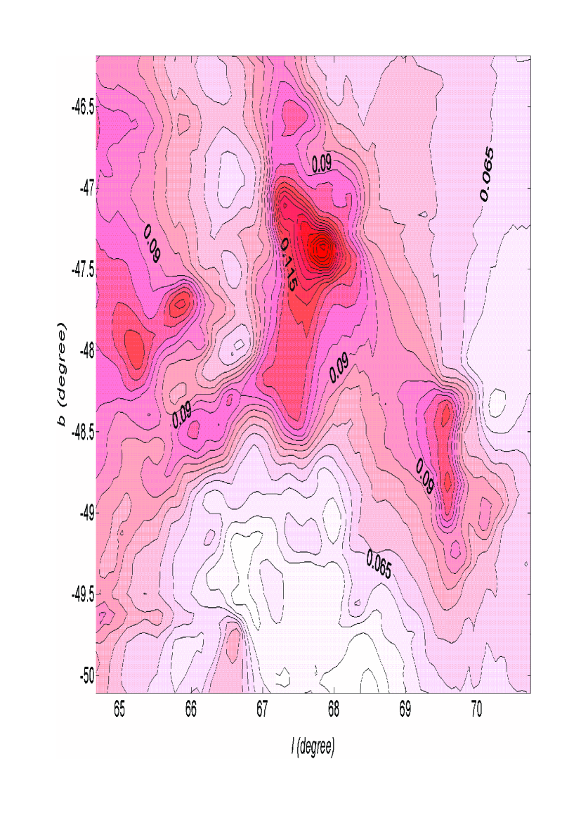
Figure 1: $E(B-V)$ colour-excess contours for the field SA 114 as a function of Galactic latitude and longitude.

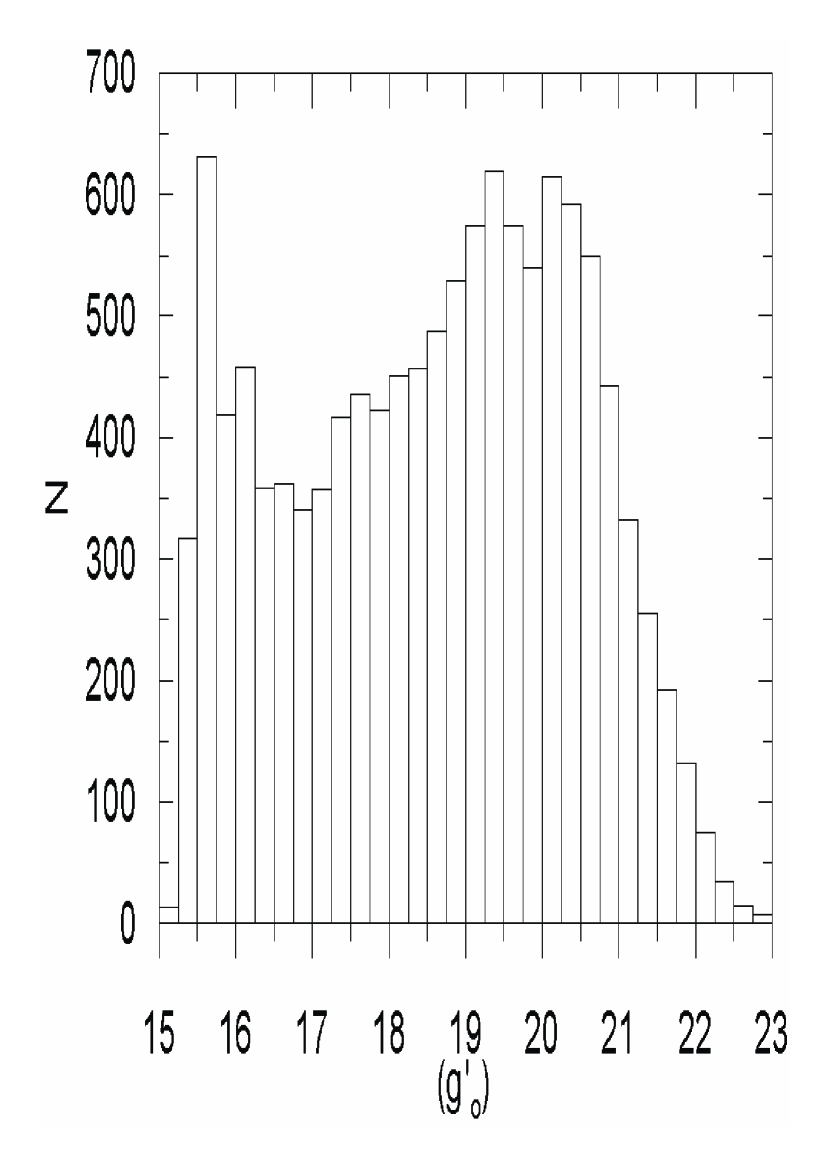
Figure 2: Apparent magnitude histogram for all sources. Bright stars are effected by saturation.

5.2 The overlapping sources, de-reddening of the magnitudes, bright stars, and extra-galactic objects

The magnitudes are provided from the Cambridge Astronomical Survey Unit (CASU). There are totally 14439 sources in 24 sub-fields in the field SA 114. It turned out that 2428 of these sources are overlapped, i.e. their angular distances are less than $1{{}^{\prime\prime}}$ to any other source. We omitted them, thus the sample reduced to 12011. The $E(B-V)$ colour-excesses for the sample sources are evaluated by the procedure of Schegel, Finkbeiner, & Davis, (1998) and corrected by the following equations of Beers et al. (2002):

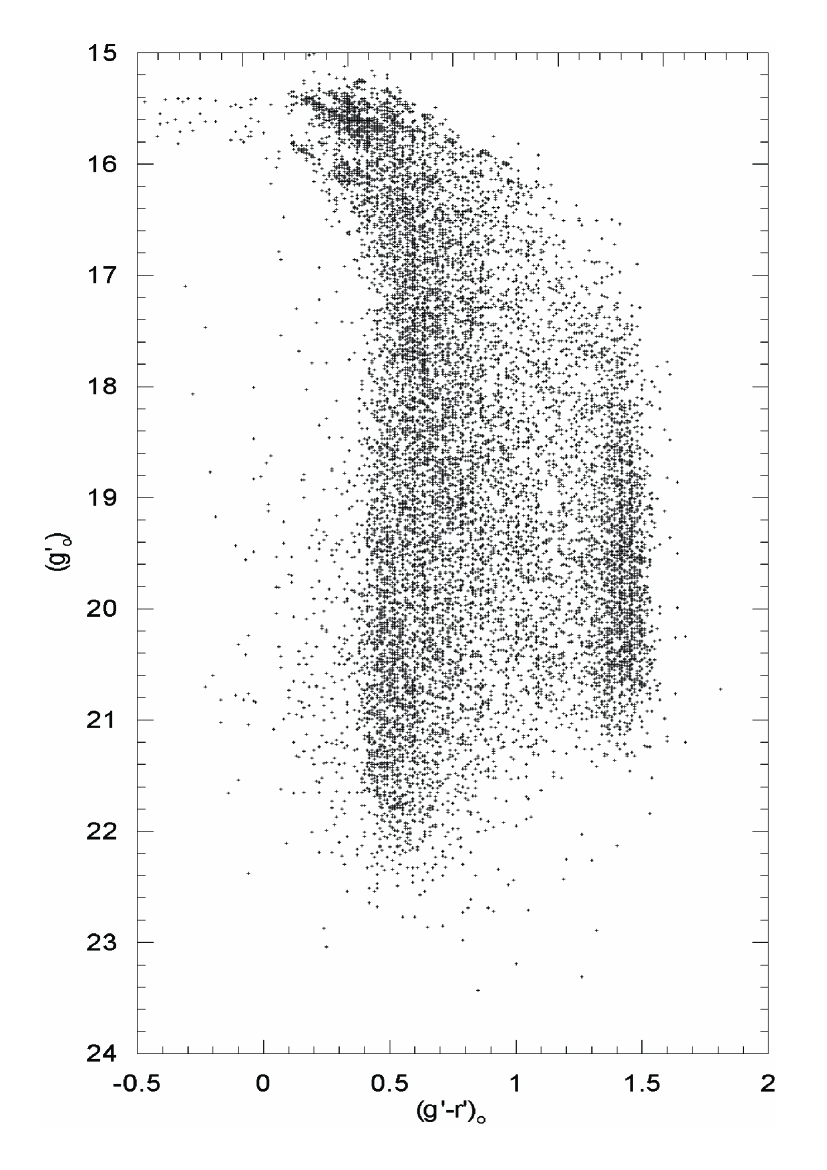
Figure 3: Colour-apparent magnitude diagram for the original sample.

$$E(B-V)=E(B-V)_{s},~{}~{}~{}~{}for~{}(B-V)s\leq 0.10$$ (11)

$$E(B-V)=0.10+0.65[E(B-V)_{s}-0.10],$$

$$~{}~{}~{}~{}for~{}E(B-V)s>0.10$$ (12)

where $E(B-V)_{s}$ is the colour-excess evaluated via the procedure of Schlegel et al. The $E(B-V)$ colour-excess contours for the field is given in Fig. 1 as a function of Galactic latitude and longitude. Then, the total absorption $A_{V}$ is evaluated by means of the well known equation,

$$R_{V}=\frac{A_{V}}{E(B-V)}=3.1$$ (13)

For Vega bands we used the $R_{\lambda}/R_{V}$ data of Cox (2000) for the interpolation, where $\lambda$ = 3581$\AA$, 4846$\AA$, 6240$\AA$, 7743$\AA$, and 8763$\AA$ (Table 2), and derived $R_{\lambda}$ by their combination with $A_{V}$. Finally, the de-reddened $u_{0}^{{}^{\prime}}$, $g_{0}^{{}^{\prime}}$, $r_{0}^{{}^{\prime}}$, $i_{0}^{{}^{\prime}}$, and $z_{0}^{{}^{\prime}}$ magnitudes were obtained from the original magnitudes and the corresponding $R_{\lambda}$.

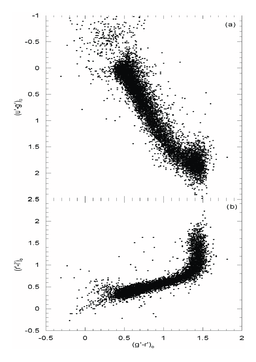
Figure 4: Two-colour diagrams for sources with apparent magnitude $17<g^{{}^{\prime}}_{0}\leq 22$. (a) for $(u^{{}^{\prime}}-g^{{}^{\prime}})_{0}-(g^{{}^{\prime}}-r^{{}^{\prime}})_{0}$ and (b) for ($g^{{}^{\prime}}-r^{{}^{\prime}})_{0}-(r^{{}^{\prime}}-i^{{}^{\prime}})_{0}$.

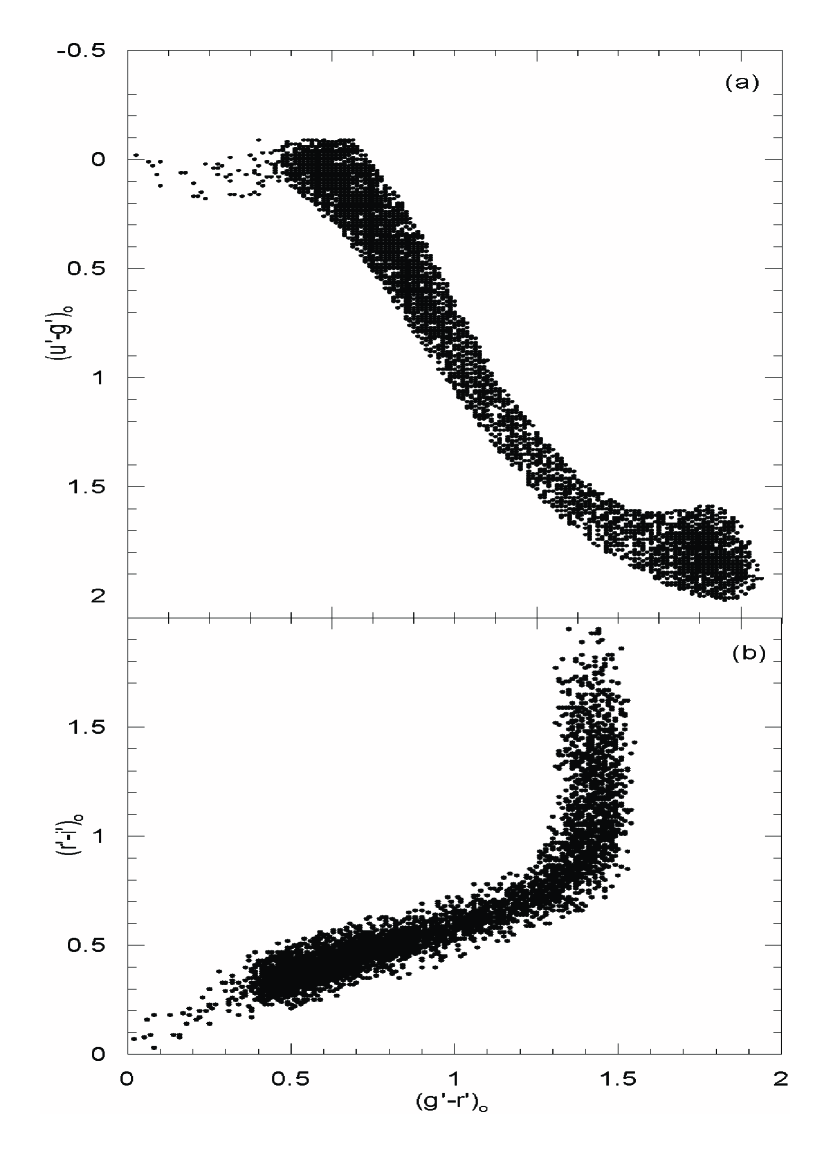
Figure 5: Two-colour diagrams for stars with apparent magnitude. $17<g^{{}^{\prime}}_{0}\leq 22$. (a) for $(u^{{}^{\prime}}-g^{{}^{\prime}})_{0}-(g^{{}^{\prime}}-r^{{}^{\prime}})_{0}$ and (b) for ($g^{{}^{\prime}}-r^{{}^{\prime}})_{0}-(r^{{}^{\prime}}-i^{{}^{\prime}})_{0}$.

Table 2: The relation between the total absorptions for Vega bands and for $V$ band of $UBV$ photometry.

Filter	$\lambda_{eff}(\AA)$	$\Delta_{eff}(\AA)$	$R_{i}/R_{v}$	$m_{lim}$
$u^{{}^{\prime}}$	3581	638	1.575	24.3
$g^{{}^{\prime}}$	4846	1285	1.164	25.2
$r^{{}^{\prime}}$	6240	1347	0.867	24.5
$i^{{}^{\prime}}$	7743	1519	0.648	23.7
$z^{{}^{\prime}}$	8763	950	0.512	22.1

The histogram for the de-reddened apparent magnitude $g_{0}^{{}^{\prime}}$ (Fig. 2) and the colour-apparent magnitude diagram (Fig. 3) show that there is a large number of saturated sources in our sample. Hence, we excluded sources brighter than $g_{0}^{{}^{\prime}}=17$. However, the two-colour diagrams $(u^{{}^{\prime}}-g^{{}^{\prime}})_{0}$ - $(g^{{}^{\prime}}-r^{{}^{\prime}})_{0}$ and $(g^{{}^{\prime}}-r^{{}^{\prime}})_{0}$ - $(r^{{}^{\prime}}-i^{{}^{\prime}})_{0}$ in Fig. 4 indicate that there are also some extra-galactic objects, where most of them lie towards the blue as claimed by Chen et al. (2001). It seems that the star/extragalactic object separation based on the ’stellarity parameter’ as returned from the SExtractor routines (Bertin & Arnouts, 1996) couldn’t be sufficient. This parameter has a value between 0 (highly extended), and 1 (point source). The separation work very well to classify a point source with a value greater than 0.8. We adopted the simulations of Fan (1999), additional to the work cited above to remove the extragalactic objects in our field. Thus we rejected the sources with $(u^{{}^{\prime}}-g^{{}^{\prime}})_{0}<-0.10$, and those which lie outside of the band concentrated by most of the sources. After the last process the number of sources in the sample, stars, reduced to 6418. The two-colour diagrams $(u^{{}^{\prime}}-g^{{}^{\prime}})_{0}$ - $(g^{{}^{\prime}}-r^{{}^{\prime}})_{0}$ and $(g^{{}^{\prime}}-r^{{}^{\prime}})_{0}$ - $(r^{{}^{\prime}}-i^{{}^{\prime}})_{0}$ for the final sample are given in Fig. 5. A few dozen of stars with $(u^{{}^{\prime}}-g^{{}^{\prime}})_{0}\sim 0.10$ and $(g^{{}^{\prime}}-r^{{}^{\prime}})_{0}\sim 0.20$ are probably stars of spectral type A.

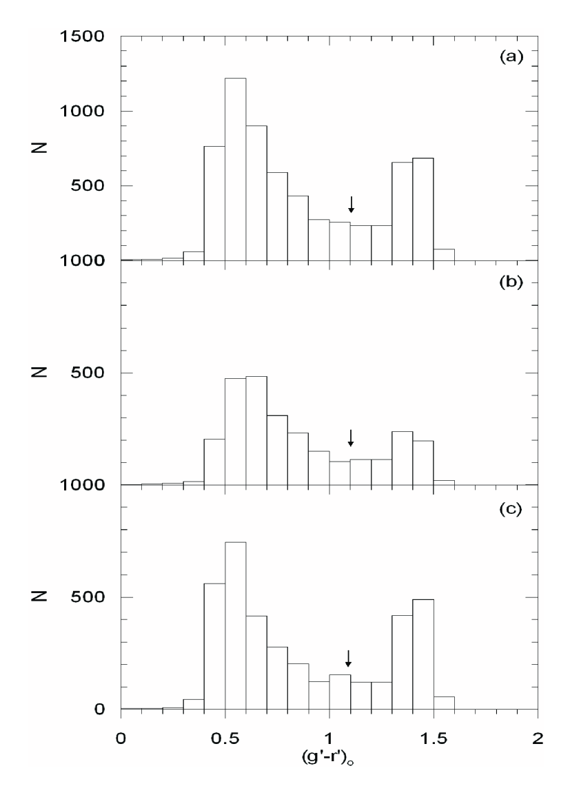
Figure 6: $(g^{{}^{\prime}}-r^{{}^{\prime}})_{0}$ colour histogram as a function of apparent magnitude, for the star sample. (a) for $17<g^{{}^{\prime}}_{0}\leq 22$, (b) for $17<g^{{}^{\prime}}_{0}\leq 19$, and (c) for $19<g^{{}^{\prime}}_{0}\leq 22$. The vertical downward arrow shows the limit value $(g^{{}^{\prime}}-r^{{}^{\prime}})_{0}=1.1$ mag which separates thin disk and thick disk - halo couple.

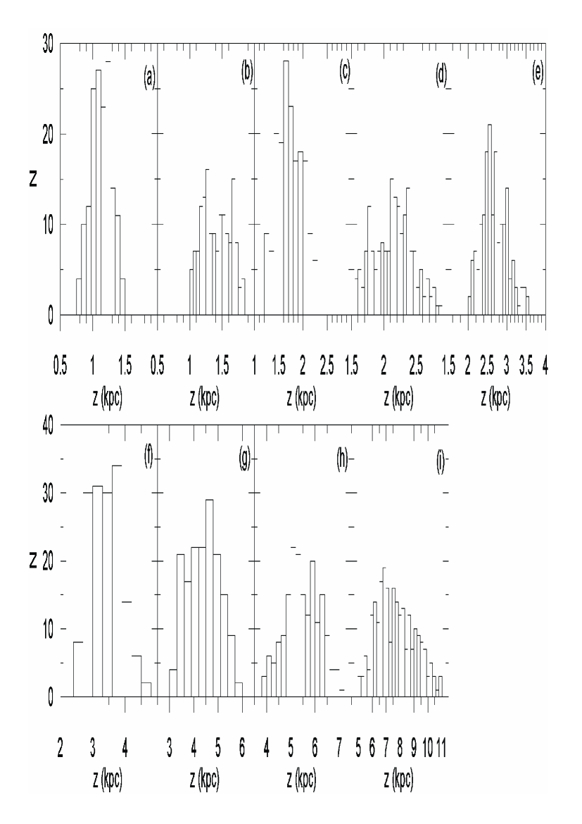
Figure 7: Spatial distribution for stars with absolute magnitude $6<M(g^{{}^{\prime}})\leq 7$ as a function of apparent magnitude. (a)(17.0-17.5], (b) (17.5-18.0], (c)(18.0-18.5], (d)(18.5-19.0], (e)(19.0-19.5], (f)(19.5-20.0], (g) (20.0-20.5], (h)(20.5-21.0], and (i) (21-22]

5.3 Absolute magnitudes, distances, population types and density functions

In the $Sloan$ photometry, the blue stars in the range $15<g^{{}^{\prime}}<18$ are dominated by thick disk stars with a turnoff $(g^{{}^{\prime}}-r^{{}^{\prime}})\sim 0.33$, and for $g^{{}^{\prime}}>18$, the Galactic halo, has a turnoff colour $(g^{{}^{\prime}}-r^{{}^{\prime}})\sim 0.2$, becomes significant. Red stars, $(g^{{}^{\prime}}-r^{{}^{\prime}})\geq 1.3$, are dominated by thin disk stars for all apparent magnitudes (Chen et al. 2001). In our case, the apparent magnitude which separates the thick disk and halo stars seems to be a bit fainter relative to the $Sloan$ photometry, i.e. $g_{0}^{{}^{\prime}}\sim 19$ (Fig. 3). Thus, stars bluer than $(g^{{}^{\prime}}-r^{{}^{\prime}})=1.1$ and brighter than $g_{0}^{{}^{\prime}}=19$ are separated to the thick disk population and the colour-magnitude diagram of 47 Tuc (Hesser et al. 1987) is used for their absolute magnitude determination, whereas those with the same colour but fainter than $g_{0}^{{}^{\prime}}=19$ are assumed to be as halo stars and their absolute magnitudes are determined via the colour-magnitude diagram of M92 (Stetson & Harris 1988). From the other hand, stars redder than $(g^{{}^{\prime}}-r^{{}^{\prime}})=1.1$ are adopted as thin disk stars and their absolute magnitudes are evaluated by means of the colour-magnitude diagram of Lang (1992) for Pop I stars (Fig. 6). The distance to a star relative to the Sun is carried out by the following formula:

$$(g^{{}^{\prime}}-M(g^{{}^{\prime}}))_{o}=5\log r-5$$ (14)

The vertical distance to the galactic plane ($z$) of a star could be evaluated by its distance $r$ and its Galactic latitude ($b$) which could be provided by its right ascension and declination. The precise separation of stars into different populations have been carried out by their spatial distribution as a function of their absolute and apparent magnitudes. Fig. 7 gives the spatial distribution of stars with $6<M(g^{{}^{\prime}})\leq 7$, as an example, and Table 3 gives the full set of absolute and apparent magnitude intervals, and the efficiency regions of the populations. Halo stars dominate the absolutely bright intervals, thick disk stars indicate the intermediate and the thin disk stars the faint ones, as expected (Fig. 8).

Number of stars as a function of distance $r$ relative to the Sun, and the corresponding mean distance $z^{*}$ from the Galactic plane, for different absolute magnitude intervals for three populations are given in Tables 4-6. The logarithmic space density functions, $D^{*}=\log D+10$, evaluated by means of these data are not given in the tables for avoidance space consuming but they are presented in Fig. 9-11, where $D=N/\Delta V_{1,2}$, $\Delta V_{1,2}=(\pi/180)^{2}(\sq/3)(r_{2}^{3}-r_{1}^{3})$, $\sq$: size of the field (4.239 square-degree), $r_{1}$ and $r_{2}$: the limiting distance of the volume $\Delta V_{1,2}$, and N: number of stars (per unit absolute magnitude). The horizontal thick lines, in Tables 4-6, corresponding to the limiting distance of completeness ($z_{l}$) are evaluated by the following equations:

Table 3: Dominant regions for three populations; thin disk, thick disk, and halo, as a function of absolute and apparent magnitudes. The symbol $z$ is the distance to the Galactic plane.

$M(g^{{}^{\prime}})$	$g_{o}^{{}^{\prime}}$	Thin disk	Thick disk	Halo
(12-13]	(17-22]	$z\leq 0.50$	$---$	$---$
(11-12]	(17-22]	$z\leq 0.80$	$---$	$---$
(10-11]	(17-22]	$z\leq 1.30$	$---$	$---$
(9-10]	(17-22]	$z\leq 1.50$	$z>1.50$	$---$
(8-9]	(17-18]	$z\leq 0.60$	$z>0.60$	$---$
	(18-19]	$z\leq 0.85$	$z>0.85$	$---$
	(19-20]	$z\leq 1.25$	$z>1.25$	$---$
	(20-22]	$z\leq 1.60$	$z>1.60$	$---$
(7-8]	(17-18]	$z\leq 1.00$	$z>1.00$	$---$
	(18-19]	$z\leq 1.30$	$z>1.30$	$---$
	(19.0-19.5]	$z\leq 1.70$	$z>1.70$	$---$
	(19.5-20.0]	$---$	$z\leq 2.55$	$z>2.55$
	(20-22]	$---$	$z\leq 3.80$	$z>3.80$
(6-7]	(17.0-17.5]	$z\leq 1.12$	$z>1.12$	$---$
	(17.5-18.0]	$z\leq 1.40$	$z>1.40$	$---$
	(18.0-18.5]	$z\leq 1.50$	$z>1.50$	$---$
	(18.5-19.0]	$z\leq 1.90$	$z>1.90$	$---$
	(19.0-19.5]	$z\leq 2.25$	$z>2.25$	$---$
	(19.5-20.0]	$---$	$z\leq 4.60$	$---$
	(20.0-20.5]	$---$	$z\leq 4.70$	$z>4.70$
	(20.5-21.0]	$---$	$z\leq 5.60$	$z>5.60$
	(21-22]	$---$	$z\leq 6.40$	$z>6.40$
(5-6]	(17.0-18.0]	$z\leq 1.68$	$z>1.68$	$---$
	(18.0-18.5]	$z\leq 2.18$	$z>2.18$	$---$
	(18.5-19.0]	$z\leq 2.52$	$z>2.52$	$---$
	(19.0-19.5]	$---$	$z\leq 4.50$	$z>4.50$
	(19.5-20.0]	$---$	$z\leq 4.50$	$z>4.50$
	(20-22]	$---$	$---$	$z>4.50$
(4-5]	(17-18]	$---$	$z\leq 2.20$	$z>2.20$
	(18-19]	$---$	$z\leq 3.60$	$z>3.60$
	(19-22]	$---$	$---$	$z>5.00$

Table 4: Number of stars as a function of distance $r$ relative to the Sun, and the corresponding mean distance $z*$ from the Galactic plane, for different absolute magnitude intervals for thin disk (distances in kpc). Horizontal thick lines correspond the limiting distance of completeness.

$M(g^{{}^{\prime}})\rightarrow$	(5-6]		(6-7]		(7-8]		(8-9]		(9-10]		(10-11]		(11-12]		(12-13]
$r_{1}-r_{2}$	$z^{*}$	N	$z^{*}$	N	$z^{*}$	N	$z^{*}$	N	$z^{*}$	N	$z^{*}$	N	$z^{*}$	N	$z^{*}$	N
0.10-0.20													0.13	30	0.12	20
0.20-0.30									0.22	4	0.19	42	0.19	115	0.19	39
0.30-0.40									0.27	21	0.26	83	0.26	129	0.26	33
0.40-0.60							0.43	59	0.37	66	0.37	154	0.36	182	0.34	28
0.60-0.80					0.56	14	0.52	65	0.52	58	0.52	158	0.50	71
0.80-1.00					0.67	43	0.68	58	0.68	72	0.67	87	0.66	20
1.00-1.25			0.87	18	0.84	87	0.82	65	0.85	72	0.83	77
1.25-1.50			1.03	67	1.02	76	1.03	55	1.03	46	1.01	30
1.50-1.75	1.26	8	1.21	60	1.21	59	1.20	66	1.20	37	1.24	7
1.75-2.00	1.42	39	1.39	46	1.40	37	1.40	16	1.40	16
2.00-2.50	1.58	75	1.71	41	1.61	57	1.53	9	1.63	9
2.50-3.00	2.08	26	2.08	21					1.99	4
3.00-3.50	2.50	11	2.24	2
Total		159		255		373		393		405		638		547		120

Table 5: Number of stars for different absolute magnitude intervals for thick disk (symbols as in Table 4).

$M(g^{{}^{\prime}})\rightarrow$	(4-5]	(5-6]	(6-7]	(7-8]	(8-9]
$r_{r}-r_{2}$	$z^{*}$   N	$z^{*}$   N	$z^{*}$   N	$z^{*}$   N	$z^{*}$   N
0.5-1.0					0.64  30
1.0-1.5	1.05  17		1.13   1	1.04  10	0.95  59
1.5-2.0	1.29  51		1.30  95	1.38  40	1.37  79
2.0-2.5	1.66  69	1.78  80	1.66 136	1.74  65	1.69  84
2.5-3.0	2.05  44	2.05 116	2.06 124	2.05  99	2.02  44
3.0-3.5	2.42  20	2.42 115	2.43 129	2.42  67	2.42  23
3.5-4.0	2.77  20	2.81 107	2.80 104	2.82  53	2.78  10
4.0-4.5	3.14  18	3.18  63	3.17  72	3.16  47	3.09   7
4.5-5.0	3.48   3	3.57  66	3.54  69	3.50  30	3.57   4
5.0-5.5		3.91  51	3.90  54	3.75   5
5.5-6.0		4.30  38	4.26  53
6.0-6.5		4.66  34	4.62  44
6.5-7.0		5.06  11	5.03  38
7.0-8.0		5.27   4	5.38  58
8.0-9.0			5.83  24
Total	242	685	1001	416	340

Table 6: Number of stars for different absolute magnitude intervals for halo (symbols as in Table 4).

$M(g^{{}^{\prime}})\rightarrow$	(4-5]		(5-6]		(6-7]		(7-8]
$r_{1}-r_{2}$	$z^{*}$	N	$z^{*}$	N	$z^{*}$	N	$z^{*}$	N
2-4	2.58	19					2.73	14
4-6	3.81	34					4.17	42
6-8	5.05	25	5.37	99	5.38	76	5.04	48
8-10	6.57	10	6.71	113	6.65	117	6.72	10
10-15	9.10	27	9.13	178	8.73	129
15-20	12.97	17	12.54	57
20-25	17.00	3	16.02	2
25-30	19.44	4
30-35	22.11	2
Total		141		449		322		114

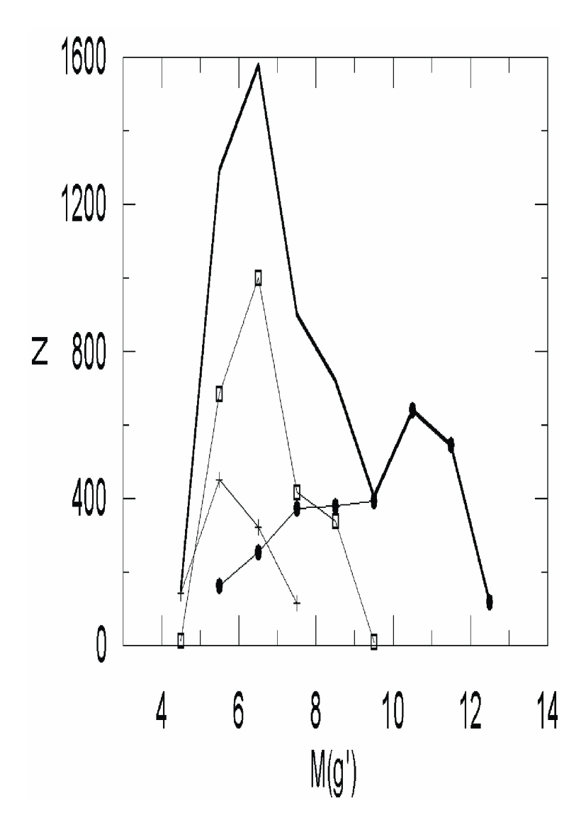
Figure 8: Absolute magnitude ranges dominated by different populations. Symbols: (+) halo, ($\sq$) thick disk, ($\bullet$) thin disk, and thick line: the distribution of stars for all absolute magnitudes

$$(g^{{}^{\prime}}-M(g^{{}^{\prime}}))_{o}=5\log r_{l}-5$$ (15)

$$z_{l}=r_{l}sinb$$ (16)

where $g_{0}^{{}^{\prime}}$ is the limiting apparent magnitude (17 and 22, for the bright and faint stars, respectively), $r_{l}$ the limiting distance of completeness relative to the Sun, and $M(g_{0}^{{}^{\prime}})$ the appropriate absolute magnitude $M_{1}$ or $M_{2}$ for the absolute magnitude interval $M_{1}-M_{2}$ considered.

Table 7: Galactic model parameters for different absolute magnitude intervals for thin disk resulting from the comparison of observed logarithmic space densities with a (unique) density law (Fig. 9). The columns give: $M(g^{{}^{\prime}})$ absolute magnitude interval, density law, logarithmic local space density $n^{*}$, scale height for $sech$ or $sech^{2}$ density law $z_{0}$, scale height for exponential density law H, $\chi^{2}$, standart deviation $s$, and local space densities for Hipparcos $\odot$.

$M(g^{{}^{\prime}})$	Density Law	$n^{*}$	$z_{o}/H$ (pc)	$\chi^{2}.(10^{-10})$	$s$	$\odot$
(12-13]	$exp$	$8.40^{+0.07}_{-0.07}$	$101^{+11}_{-7}$	4362816	$\pm$ 0.14	8.05
	$sech$	$8.14^{+0.07}_{-0.07}$	$98/162^{+17}_{-13}$	3767270	0.14
	$sech^{2}$	$8.08^{+0.06}_{-0.06}$	$166/275^{+22}_{-22}$	2691626	0.12
(11-12]	$exp$	$8.98^{+0.02}_{-0.05}$	$103^{+3}_{-4}$	1940921	0.10	7.92
	$sech$	$8.69^{+0.04}_{-0.04}$	$102/169^{+7}_{-5}$	1690410	0.09
	$sech^{2}$	$8.55^{+0.02}_{-0.03}$	$188/312^{+6}_{-9}$	755904	0.06
(10-11]	$exp$	$8.38^{+0.04}_{-0.04}$	$168^{+7}_{-6}$	628271	0.10	7.78
	$sech$	$8.11^{+0.03}_{-0.06}$	$168/278^{+9}_{-16}$	857229	0.10
	$sech^{2}$	$7.99^{+0.04}_{-0.04}$	$300/497^{+23}_{-21}$	994846	0.06
(9-10]	$exp$	$7.60^{+0.05}_{-0.05}$	$264^{+14}_{-13}$	274519	0.10	7.63
	$sech$	$7.34^{+0.05}_{-0.05}$	$256/424^{+24}_{-21}$	295956	0.06
	$sech^{2}$	$7.23^{+0.06}_{-0.06}$	$460/762^{+50}_{-41}$	370010	0.06
(8-9]	$exp$	$7.47^{+0.07}_{-0.06}$	$292^{+22}_{-13}$	247010	0.13	7.52
(7-8]	$exp$	$7.50^{+0.02}_{-0.02}$	$312^{+3}_{-4}$	8207	0.02	7.48
(6-7]	$exp$	$7.43^{+0.02}_{-0.02}$	$326^{+5}_{-5}$	6295	0.03	7.47
(5-6]	$exp$	$7.43^{+0.01}_{-0.01}$	$334^{+2}_{-2}$	162	0.01	7.47

6 Galactic model parameters

6.1 Density laws for different populations and different absolute magnitudes: new approach for the model parameter estimation

In the literature different density laws, such as secans hyperbolicus ($sech$), squared secans hyperbolicus ($sech^{2}$) or exponentials, were used for parameterization of thin disk data, whereas the exponential density law was sufficient for thick disk data. In the present study, we compared the observed logarithmic space densities for thin disk with all density laws cited above. It turned out that $sech^{2}$ law fits better for three faint absolute magnitude intervals, i.e. $12<M(g^{{}^{\prime}})\leq 13$, $11<M(g^{{}^{\prime}})\leq 12$, and $10<M(g^{{}^{\prime}})\leq 11$, whereas exponential law is favourable for brighter absolute magnitudes (Table 7 and Fig. 9). The argument used for this conclusion is the difference between the local space density resulting from the comparison of the observed space density functions with the density laws and the Hipparcos one (Jahreiss & Wielen 1997). Table 7 gives also the corresponding scale-heights. It is interesting, the scale-height increase monotonously when one goes from the faint magnitudes towards the bright ones, however there is a discontunity at the transition region of two density laws. The range and the mean of the scale-height for thin disk are 264-497 pc, and 327 pc, respectively. Although 497 pc seems an extreme value, it is close to the upper limit cited by Robin & Crézé (1986).

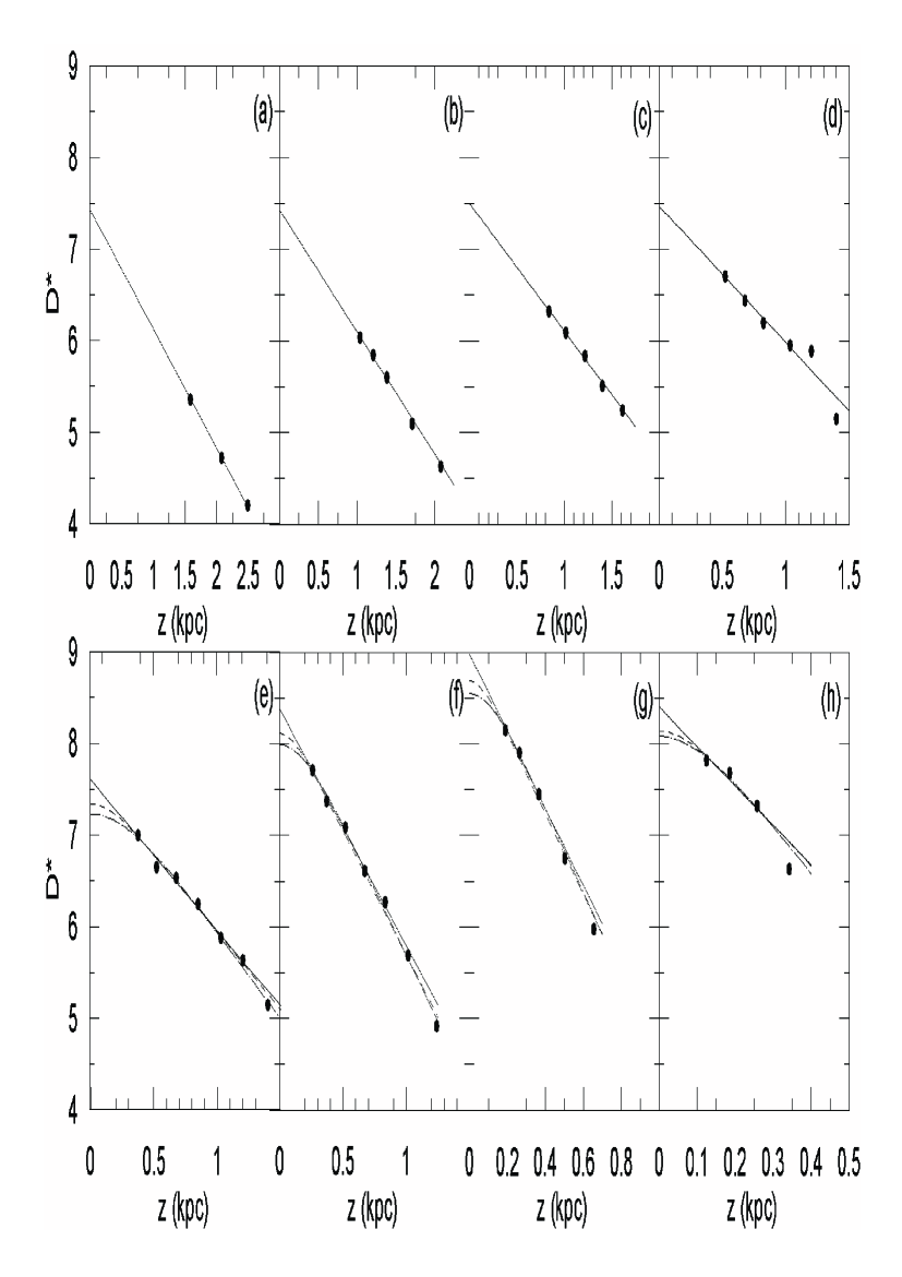
Figure 9: Comparison of the observed space density function with the density laws for different absolute magnitude intervals for the thin disk. (a) (5-6], (b) (6-7], (c) (7-8], (d) (8-9], (e) (9-10], (f) (10-11], (g) (11-12], and (h) (12-13]. Continuous curve: represents exponential law, whereas dashed curve, $sech$ law and dashed-dot curve, $sech^{2}$ law.

Table 8: Galactic model parameters for thick disk. $n_{2}/n_{1}$ indicates the local space density for thick disk relative to thin disk. Other symbols are same as in Table 7.

$M(g^{{}^{\prime}})$	$n^{*}$	$z_{o}/H$ (pc)	$\chi^{2}.(10^{-10})$	$s$	$n_{2}/n_{1}(\%)$
(8-9]	$6.19^{+0.01}_{-0.01}$	$970^{+27}_{-29}$	2002	$\pm$ 0.02	5.25
(7-8]	$6.31^{+0.07}_{-0.08}$	$806^{+52}_{-47}$	18505	0.07	6.46
(6-7]	$6.42^{+0.03}_{-0.03}$	$895^{+18}_{-23}$	5879	0.06	9.77
(5-6]	$6.41^{+0.04}_{-0.04}$	$876^{+26}_{-25}$	5503	0.08	9.55

Table 9: Galactic model parameters for halo. $\kappa$ and $n_{3}/n_{1}$ give the axial ratio and the local space density for halo relative to thin disk, respectively. Other symbols are as in Table 7.

$M(g^{{}^{\prime}})$	$n^{*}$	$\kappa$	$\chi^{2}.(10^{-10})$	$s$	$n_{3}/n_{1}(\%)$
(7-8]	$3.98^{+0.15}_{-0.14}$	$0.78^{+0.22}_{-0.18}$	1959	$\pm$ 0.30	0.02
(6-7]	$4.27^{+0.10}_{-0.11}$	$0.71^{+0.10}_{-0.08}$	778	0.13	0.07
(5-6]	$4.53^{+0.06}_{-0.06}$	$0.57^{+0.03}_{-0.03}$	271	0.14	0.13
(4-5]	$4.79^{+0.07}_{-0.06}$	$0.26^{+0.01}_{-0.01}$	189	0.16	0.31

For the thick disk, the observed logarithmic space density functions are compared with the exponential density law for the absolute magnitude intervals $8<M(g^{{}^{\prime}})\leq 9$, $7<M(g^{{}^{\prime}})\leq 8$, $6<M(g^{{}^{\prime}})\leq 7$, and $5<M(g^{{}^{\prime}})\leq 6$ (Table 8, Fig. 10). The scale-height for different absolute magnitude intervals varies from 806 pc to 970 pc and are in agreement with the recent values in the cited literature (see the references in Table 1). The local space density relative to the one of thin disk, for the corresponding absolute magnitude intervals in Table 7, increases from the faint absolute magnitudes to the bright ones in a range (5.25-9.77)%, again in agreeable with the literature. The observed logarithmic space density functions for halo have been compared with the de Vaucouleurs density law for the absolute magnitude intervals $7<M(g^{{}^{\prime}})\leq 8$, $6<M(g^{{}^{\prime}})\leq 7$, $5<M(g^{{}^{\prime}})\leq 6$, and $4<M(g^{{}^{\prime}})\leq 5$ (Table 9 and Fig. 11). The axial ratio decreases from relative absolute magnitudes to the bright ones, whereas the local space density relative to the thin disk for the corresponding absolute magnitude intervals increases in the same order. The parameters cited here are in the range given in the literature, except the ones for the interval $4<M(g^{{}^{\prime}})\leq 5$. The parameters derived for three populations have been tested by the luminosity function, given in Table 10 and Fig. 12, where $\varphi^{*}(M)$ is the total of the local space densities for three populations. There is a good agreement between our luminosity function and that of Hipparcos (Jahreiss & Wielen 1997) with the exception of absolute magnitude interval $11<M(g^{{}^{\prime}})\leq 12$. Also, the corresponding standard deviations for all intervals are small (Table 10).

Table 10: Luminosity function resulting from the combination of local space densities for three populations, i.e. thin and thick disks, and halo, taken from Tables 7-9. The luminosity function of Hipparcos is given in the last column.

$M(g^{{}^{\prime}})$	$\varphi^{*}(M)$	$s$	$\odot$
(12-13]	8.08	$\pm$0.14	8.05
(11-12]	8.55	0.10	7.92
(10-11]	7.99	0.10	7.78
(9-10]	7.60	0.10	7.63
(8-9]	7.49	0.13	7.52
(7-8]	7.53	0.02	7.48
(6-7]	7.47	0.03	7.47
(5-6]	7.47	0.01	7.47

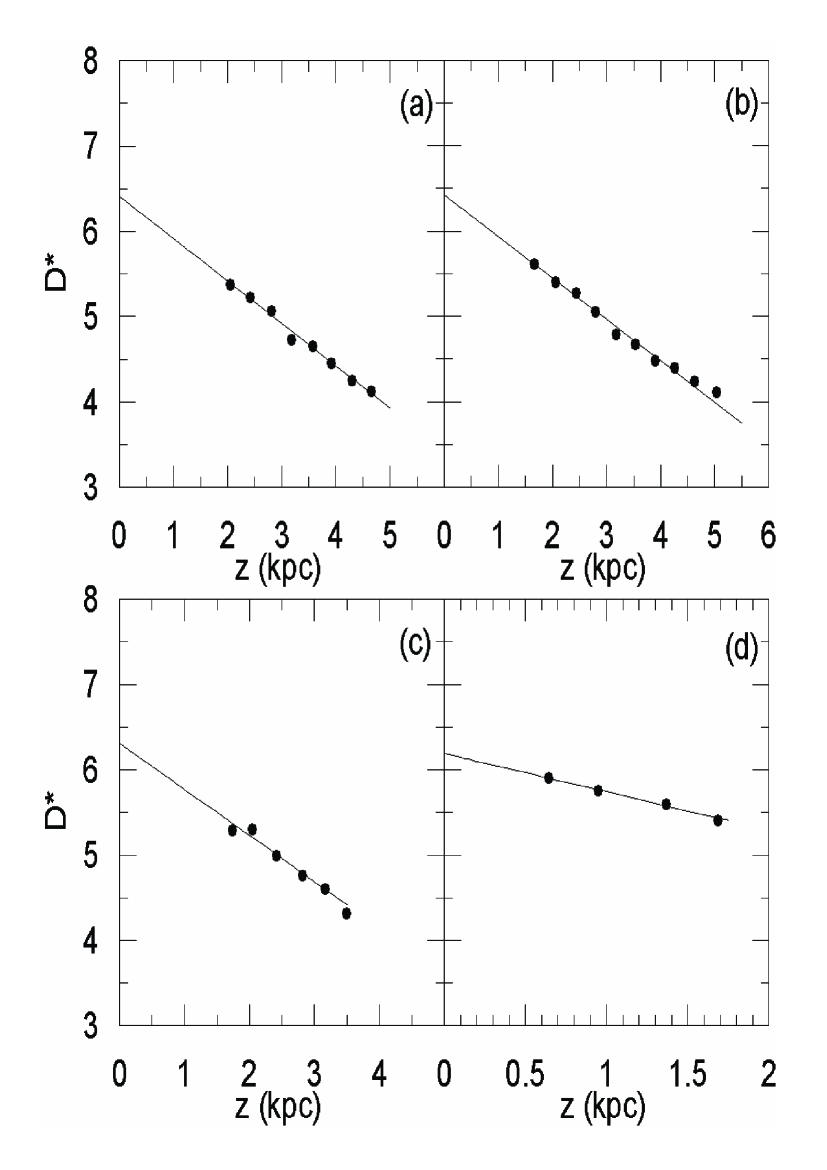
Figure 10: Comparison of the observed space density function with the exponential density law for different absolute magnitude intervals for thick disk. (a) (5-6], (b) (6-7], (c) (7-8], and (d) (8-9].

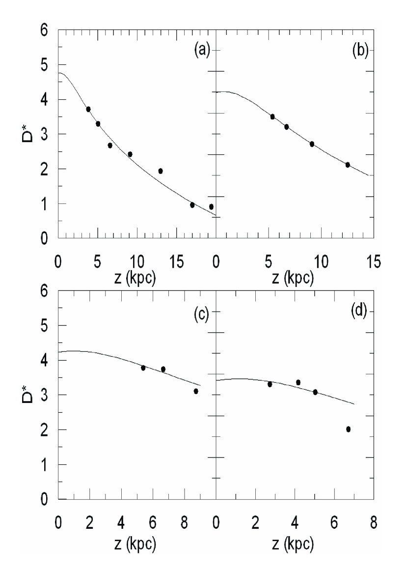
Figure 11: Comparison of the observed space density function with the de Vaucouleurs density law for different absolute magnitude intervals for halo. (a) (4-5], (b) (5-6], (c) (6-7], and (d) (7-8].

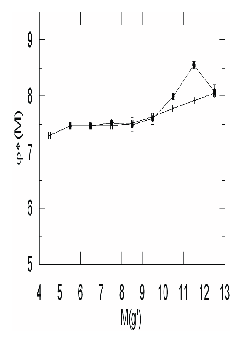
Figure 12: Luminosity function obtained from combination of the local space densities for thin and thick disks and halo, resulting from comparison of the observed space density function with the density laws, for different absolute magnitude intervals. (H) shows the Hipparcos values.

We used the procedure of Phleps et al. (2000) for the error estimation in Tables 7-9 (above) and Tables 12 and 14 (in the following sections), i.e. by changing the values of the parameters until $\chi^{2}$ increases or decreases by 1.

6.2 Model parameter estimation by the procedure in situ

We estimated the local space density and scale-height for thin disk and thick disk, and the local space density and axial ratio for halo simultaneously by the procedure in situ, i.e. by comparison of the combined observed space density functions with the combined density laws. We carried out this work for two sets of absolute magnitude intervals, $5<M(g^{{}^{\prime}})\leq 10$ and $5<M(g^{{}^{\prime}})\leq 13$. The second set covers the thin disk stars with $10<M(g^{{}^{\prime}})\leq 13$ whose density functions behave differently than the density functions for stars with other absolute magnitudes. Number of stars as a function of distance $r$ relative to the Sun for eight absolute magnitude intervals are given in Table 11 and the density functions per unit absolute magnitude interval evaluated by these data are shown in Table 12 and Table 13 for the sets $5<M(g^{{}^{\prime}})\leq 10$ and $5<M(g^{{}^{\prime}})\leq 13$, respectively.

6.2.1 Model parameters by means of absolute magnitudes $5<M(g^{{}^{\prime}})\leq 10$

The observed space densities per absolute magnitude interval for three populations, i.e. thin and thick disks, and halo for stars with $5<M(g^{{}^{\prime}})\leq 10$, (Table 12) are compared with the combined density laws in situ (Fig. 13). The derived parameters are given in Table 14. All these parameters are in agreement with the ones given in Table 1. Especially the relative local space density for thick disk, 8.32%, lies within the range given in two recent works (Chen et al. 2001 and Siegel et al. 2002). The resulting luminosity function (Fig. 14) from the comparison of the model with these parameters and the combined observed density functions per absolute magnitude interval is also in agreement with the one of Hipparcos (Jahreiss & Wielen 1997). However the error bars are longer than the ones in Fig. 12, particularly for the faint magnitudes.

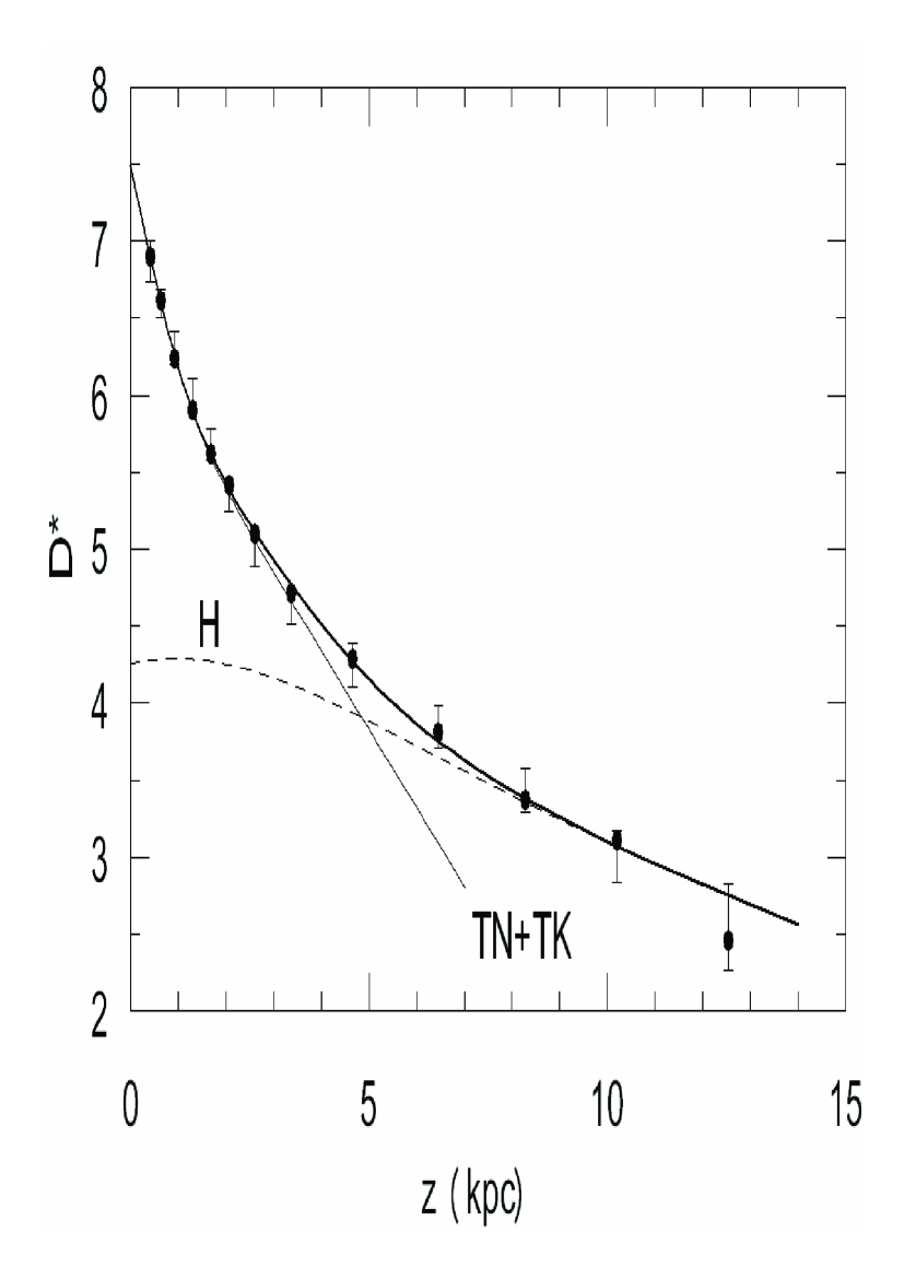
Figure 13: Comparison of the observed space density function combined for thin and thick disks and halo with the combined density law, for stars with $5<M(g^{{}^{\prime}})\leq 10$.

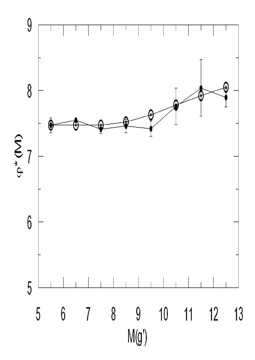
Figure 14: Luminosity function resulting from the comparison of the combined observed space density function with the combined density law, for stars with $5<M(g^{{}^{\prime}})\leq 10$.

Table 11: Number of stars as a function of distance $r$ relative to the Sun, and the corresponding mean distance $z^{*}$ from the Galactic plane, for different absolute magnitude intervals (distances in kpc). Horizontal thick lines correspond the limiting distance of completeness.

$M(g^{{}^{\prime}})\rightarrow$	(5-6]		(6-7]		(7-8]		(8-9]		(9-10]		(10-11]		(11-12]		(12-13]
$r_{1}-r_{2}$	$z^{*}$	N	$z^{*}$	N	$z^{*}$	N	$z^{*}$	N	$z^{*}$	N	$z^{*}$	N	$z^{*}$	N	$z^{*}$	N
0.0-0.2										0.15	1	0.13	30	0.12	20
0.2-0.4									0.26	25	0.24	125	0.23	244	0.22	72
0.4-0.7							0.45	77	0.41	96	0.41	236	0.39	230	0.34	28
0.7-1.0					0.65	57	0.63	135	0.64	100	0.62	163	0.59	41
1.0-1.5			1.00	86	0.93	173	0.93	179	0.92	118	0.89	109	0.75	2
1.5-2.0	1.39	47	1.29	201	1.32	136	1.30	149	1.26	53	1.27	4
2.0-2.5	1.69	158	1.68	177	1.68	122	1.67	93	1.63	9
2.5-3.0	2.06	142	2.06	145	2.05	99	2.02	44	1.99	4
3.0-4.0	2.60	233	2.59	235	2.61	134	2.53	33
4.0-5.0	3.38	129	3.35	141	3.29	77	3.21	10
5.0-7.5	4.63	209	4.68	284	4.54	91	3.81	1
7.5-10.0	6.53	141	6.40	181	6.42	14
10.0-12.5	8.28	100	8.27	93
12.5-15.0	10.21	78	9.90	36
15.0-20.0	12.54	57
20.0-25.0	16.02	2
Total		1296		1579		903		721		405		638		547		120

6.2.2 Model Parameters by means of absolute magnitudes $5<M(g^{{}^{\prime}})\leq 13$

We carried out the work cited in the previous paragraph for stars with a larger range of absolute magnitude, i.e. $5<M(g^{{}^{\prime}})\leq 13$. The observed density function is given in Table 13 and its comparison with the combined density law is shown in Fig. 15. The derived parameters (Table 15), especially the local densities, are rather different than the ones cited in Sections (6.1) and (6.2.1). The reason for this discrepancy is that stars with absolute magnitudes $10<M(g^{{}^{\prime}})\leq 13$ have relatively larger local space densities (Hipparcos; Jahreiss & Wielen 1997) and are closer to the Sun relative to stars brighter than $M(g^{{}^{\prime}})$=10, and they affect the combined density function considerably. Also the corresponding luminosity function is not in agreement with the one of Hipparcos, except one absolute magnitude interval, $12<M(g^{{}^{\prime}})\leq 13$ (Fig. 16).

Table 12: Logarithmic space density function, $D^{*}=\log D+10$, per unit absolute magnitude interval for stars with $5<M(g^{{}^{\prime}})\leq 10$. $<N>$ is the weighted mean of number of stars for the absolute magnitude intervals in Table 11 under consideration, the other symbols are explained in the text (distances in kpc, volumes in pc³).

$r_{1}-r_{2}$	$\Delta V_{1,2}$	$z^{*}$	$<N>$	$D^{*}$
0.4-0.7	1.20 (5)	0.408	96	6.90
0.7-1.0	2.83 (5)	0.634	118	6.62
1.0-1.5	1.02 (6)	0.929	176	6.24
1.5-2.0	1.99 (6)	1.302	162	5.91
2.0-2.5	3.28 (6)	1.678	138	5.62
2.5-3.0	4.90 (6)	2.055	129	5.42
3.0-4.0	1.59 (7)	2.600	201	5.10
4.0-5.0	2.63 (7)	3.365	135	4.71
5.0-7.5	1.28 (8)	4.656	247	4.29
7.5-10.0	2.49 (8)	6.457	161	3.81
10.0-12.5	4.10 (8)	8.279	97	3.37
12.5-15.0	6.12 (8)	10.208	78	3.11
15.0-20.0	1.99 (9)	12.536	57	2.46

Table 13: Logarithmic space density function, $D^{*}=\log D+10$, per unit absolute magnitude interval for stars with $5<M(g^{{}^{\prime}})\leq 13$. $<N>$ is the weighted mean of number of stars for the absolute magnitude intervals in Table 11 under consideration, the other symbols are explained in the text (distances in kpc, volumes in pc³).

$r_{1}-r_{2}$	$\Delta V_{1,2}$	$z^{*}$	$<N>$	$D^{*}$
0-0.2	3.44 (3)	0.127	25	7.86
0.2-0.4	2.41 (4)	0.230	147	7.79
0.4-0.7	1.20 (5)	0.402	187	7.19
0.7-1.0	2.83 (5)	0.628	133	6.67
1.0-1.5	1.02 (6)	0.929	176	6.24
1.5-2.0	1.99 (6)	1.302	162	5.91
2.0-2.5	3.28 (6)	1.678	138	5.62
2.5-3.0	4.90 (6)	2.055	129	5.42
3.0-4.0	1.59 (7)	2.600	201	5.10
4.0-5.0	2.63 (7)	3.365	135	4.71
5.0-7.5	1.28 (8)	4.656	247	4.29
7.5-10.0	2.49 (8)	6.457	161	3.81
10.0-12.5	4.10 (8)	8.279	97	3.37
12.5-15.0	6.12 (8)	10.208	78	3.11
15.0-20.0	1.99 (9)	12.536	57	2.46

Table 14: Galactic model parameters estimated by comparison of the logarithmic space density function for stars with $5<M(g^{{}^{\prime}})\leq 10$ (given in Table 12) and the combined density laws (Fig.13). The symbols give: $n^{*}$: logaritmic local space density, H: scale height, $n/n_{1}$: local space density relative thin disk, and $\kappa$= c/a: axial ratio for halo.

Parameter	Thin disk	Thick disk	Halo
$n^{*}$	$7.46^{+0.02}_{-0.02}$	$6.38^{+0.03}_{-0.03}$	$4.30^{+0.29}_{-0.45}$
$H$ (pc)	$275^{+6}_{-5}$	$851^{+43}_{-41}$	$--$
$n/n_{1}($%$)$	$--$	$8.32$	$0.07$
$\kappa$	$--$	$--$	$0.67^{+0.33}_{-0.23}$

Table 15: Galactic model parameters estimated by comparison of the logarithmic space density function for stars with $5<M(g^{{}^{\prime}})\leq 13$ (given in Table 13) and the combined density laws (Fig. 14). Symbols as in Table 14.

Parameter	Thin disk	Thick disk	Halo
$n^{*}$	8.21	6.22	4.30
$H$ (pc)	184	1048	$--$
$n/n_{1}($%$)$	$--$	1.00	$0.01$
$\kappa$	$--$	$--$	0.67

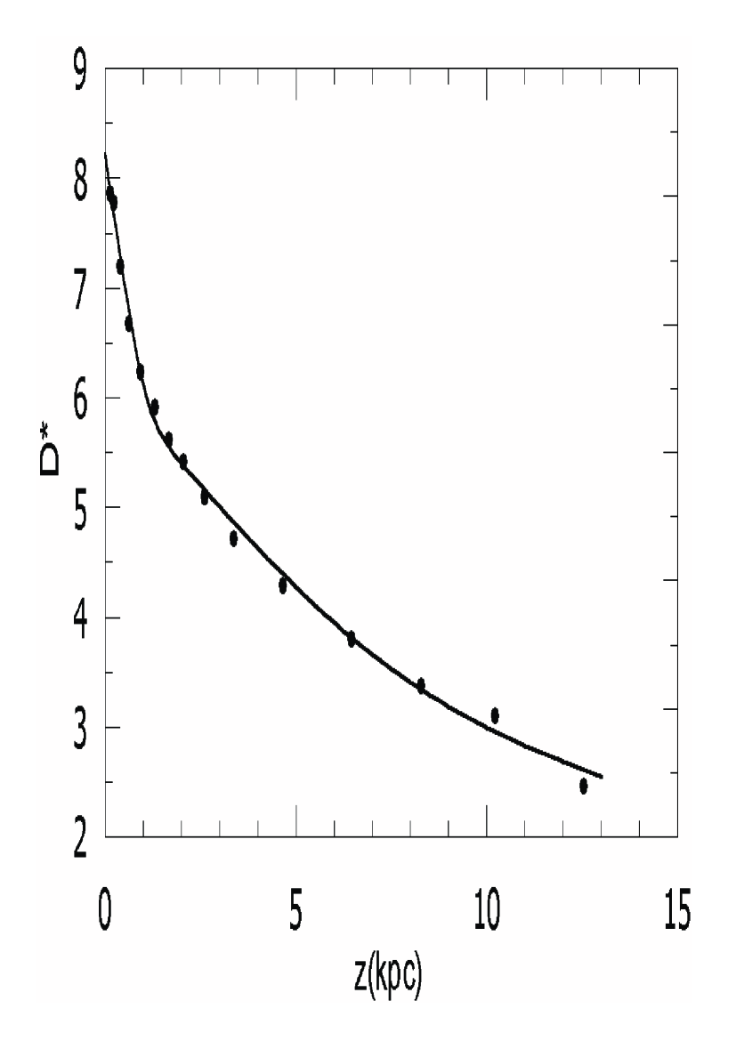
Figure 15: Comparison of the observed space density function combined for thin and thick disks and halo with the combined density laws, for stars with $5<M(g^{{}^{\prime}})\leq 13$.

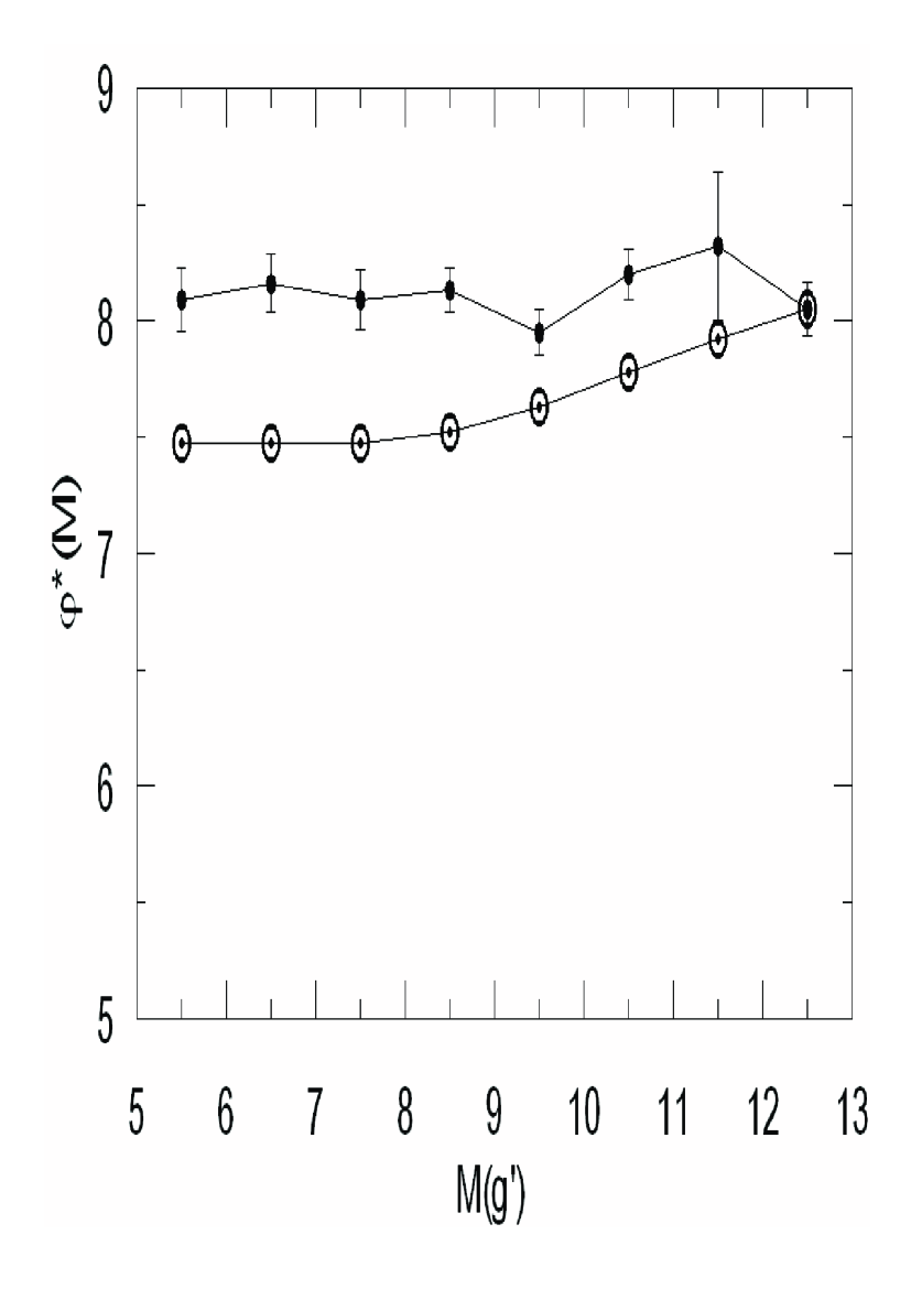
Figure 16: Luminosity function resulting from the comparison of the combined observed space density function with the combined density law, for stars with $5<M(g^{{}^{\prime}})\leq 13$.

7 Discussion

We estimated the Galactic model parameters by means of the vertical density distribution for the field SA 114 ($\alpha=22^{h}40^{m}00^{s},\delta=00^{o}00^{{}^{\prime}}00{{}^{\prime\prime}}$; $l=68^{o}.15$, $b=-48^{o}.38$; 4.239 square-degree; epoch 2000) by means of two procedures, i.e. a new approach and the procedure in situ. The new approach is based on the comparison of the observed space density functions per absolute magnitude interval with a unique density law for each population individually, where the separation of stars into different population types is carried out by a slight modification of the method of Karaali (1994), i.e. by their spatial distribution as a function of absolute and apparent magnitude. This approach covers nine absolute magnitude intervals, i.e. $4<M(g^{{}^{\prime}})\leq 5$, $5<M(g^{{}^{\prime}})\leq 6$, $6<M(g^{{}^{\prime}})\leq 7$, $7<M(g^{{}^{\prime}})\leq 8$, $8<M(g^{{}^{\prime}})\leq 9$, $9<M(g^{{}^{\prime}})\leq 10$, $10<M(g^{{}^{\prime}})\leq 11$, $11<M(g^{{}^{\prime}})\leq 12$, and $12<M(g^{{}^{\prime}})\leq 13$. Whereas the procedure in situ compares the observed space density functions per absolute magnitude interval with the combination of a set of density law representing all the populations. This procedure is carried out for two absolute magnitude intervals, $5<M(g^{{}^{\prime}})\leq 10$ and $5<M(g^{{}^{\prime}})\leq 13$. However, we will not discuss the parameters for $5<M(g^{{}^{\prime}})\leq 13$, since they are rather different than the parameters appeared in the literature up to now.

7.1 Parameters determined by means of the new approach

The new approach provides absolute magnitude dependent Galactic model parameters. The scale-height for thin disk increases monotonously from the faint magnitudes to bright ones, however there is a discontunity at the transition region of two density laws (exponential law for $M(g^{{}^{\prime}})\leq 10$, and $sech^{2}$ law for $10<M(g^{{}^{\prime}})\leq 13$). The range of this parameter is 264-497 pc, and one can find all the values derived for different absolute magnitude intervals in the literature including the extreme one, i.e. 497 pc which is close to the one cited by Robin & Crézé (1986). The thick disk is dominant in the intervals $5<M(g^{{}^{\prime}})\leq 6$, $6<M(g^{{}^{\prime}})\leq 7$, $7<M(g^{{}^{\prime}})\leq 8$, and $8<M(g^{{}^{\prime}})\leq 9$. The scale height for thick disk lies within 806-970 pc and the range of the local space density relative to the thin disk for the corresponding absolute magnitude interval is (5.25-9.77)%, in agreement with the literature. The halo population is dominant in the intervals $4<M(g^{{}^{\prime}})\leq 5$ , $5<M(g^{{}^{\prime}})\leq 6$, $6<M(g^{{}^{\prime}})\leq 7$, and $7<M(g^{{}^{\prime}})\leq 8$. The local space density and the axial ratio for the brightest interval are rather different than the ones in the other intervals and those cited up to now, this is probably due to less stars at large distances (see Table 6 and Table 9). For the other absolute magnitude intervals the relative local space density, ranging from 0.02% to %0.13, and the axial ratio with range 0.57-0.78 are also in agreement with the literature. The agreement of the luminosity function, derived by the combination of the local space densities for three populations, with the Hipparcos one is confirmation for the Galactic model parameters.

7.2 Parameters determined by means of the procedure in situ

Let us reiterate the parameters derived by means of stars with $5<M(g^{{}^{\prime}})\leq 10$. The scale-heights for thin and thick disks are 275 pc and 851 pc respectively, the axial ratio for halo is 0.67, and the local space densities for thick disk and halo, relative to the thin disk, are 8.32% and 0.07% respectively. These values are close to at least one, but not to all, of the values estimated for different absolute magnitude intervals by means of new approach (see Section 7.1 and Table 7). For example, the scale height 275 pc mentioned here is comparable with the scale height for thin disk estimated for the interval $8<M(g^{{}^{\prime}})\leq 9$, and all the parameters estimated via the procedure in situ are close to the corresponding ones estimated for the interval $8<M(g^{{}^{\prime}})\leq 9$ by means of the new procedure. Also, these values are in agreement with the parameters cited in the literature.

Although the errors are larger, the luminosity function resulting from the comparison of the observed space density functions with the Galactic model with the parameters cited above agree with the luminosity function of Hipparcos (Jahreiss & Wielen 1997), confirming the parameters.

Table 16: The most appropriate Galactic model parameters (symbols as given in the previous tables).

	Thin disk		Thick disk		Halo
$M(g^{{}^{\prime}})$	H (pc)	$n^{*}_{1}$	H (pc)	$n_{2}/n_{1}(\%)$	$\kappa$	$n_{3}/n_{1}(\%)$	$\odot$
(5-6]	335	7.4	875	9.5	0.6	0.15	7.43
(6-7]	325	7.4	895	9.8	0.7	0.05	7.47
(7-8]	310	7.5	805	6.5	0.8	0.02	7.48
(8-9]	290	7.5	970	5.2			7.52
(9-10]	265	7.6					7.63
(10-11]	495	8.0					7.78
(11-12]	310	8.6					7.92
(12-13]	275	8.1					8.05

7.3 How can we decide on the most appropriate Galactic model parameters?

We estimated different sets of Galactic model parameters in two different ways, which both are in agreement with the ones appeared so far but differ from one another, when a specific one is considered. Now the question is: can we select the most appropriate model parameters for our Galaxy? We emphasize that the model parameters are absolute - and hence mass - dependent. Also, absolutely faint stars do not contribute to thick disk and halo populations in the solar neighbourhood. Any procedure not regarding these two arguments will result in the estimation of model parameters with large range and very likely will differ with the previously cited ones, depending on the absolute magnitude interval.

The dependence of the model parameters on absolute magnitude can be explained as such; from the astrophysical point of view, the mass of a star and also its chemical composition is two of the fundamental parameters during its formation. Hence there is a good correlation between the mass of a main sequence star and its absolute magnitude, this in turn is also reflected in its spectral type. Therefore, dependence of a model parameters on absolute magnitude is expected. Particularly, if we consider the local space density of a thick disk population within the local volume, same number of stars with different magnitudes are not expected to exist. According to Fig. 8, the thick disk is mostly dominant by the stars in absolute magnitude interval of $6<M(g^{{}^{\prime}})\leq 7$. If for different magnitude intervals, the same density law is used, then we can expect to get the highest relative local space density within the thick disk for the above given interval. Actually, the last column of Table 8 collaborates our expectation, where the highest relative local space density, which is 9.77% and the lowest relative local space density, which is 5.25%, correspond to absolute magnitude interval of $6<M(g^{{}^{\prime}})\leq 7$. The same holds for other model parameters when, for instance scale height is considered. Let us consider the thin disk. This population is dominant in faint magnitudes. For instance, since at late spectral types where stellar masses for the main-sequence stars are relatively small and as they occupy the space close to the Galactic plane, one would expect short scale heights for these absolute magnitude intervals, whereas one expects large scale height for the ones corresponding to relatively bright absolute magnitude intervals. This is also the case in our work and is given in Table 7. When local space density for thin and thick disks, and for halo or for their both combination is considered, dependence of model parameters on absolute magnitude would be a result of the luminosity functions adopted up to now for individual populations.

Some researchers restrict their work related with the Galactic model estimation with absolute magnitude. The recent work of Robin et al. (2003) who treated stars with $M(V)\leq 8$ can be given as an example. This is in confirmity with our work. Finally, we argue that the most appropriate Galactic model parameters are those estimated for individual absolute magnitude intervals by comparison of the observed space density functions with the corresponding (and unique) density law. Our results obtained by this procedure are given in Table 16.

References

- [1] Buser R., Rong J., Karaali S., 1998, A&A, 331, 934 (BRK)
- [2] Buser R., Rong J., Karaali S., 1999, A&A, 348, 98
- [3] Beers T.C., Sommer-Larsen J., 1995, ApJS, 96, 175
- [4] Beers T.C., Drilling J.S., Rossi S., Chiba M., Rhee J., Fuhrmeister B., Norris J.E., von Hippel T., 2002, AJ, 124, 931
- [5] Bertin A., Arnouts S., 1996, A&AS, 117, 393
- [6] Carney B.W., Latham D.W., Laird J.B., 1990, AJ, 99, 572
- [7] Chen B., Stoughton C., Smith J.A., Uomoto A., Pier J.R., Yanny B., Ivezic Z., York D.G., Anderson J.E., Annis J., Brinkmann J., Csabai I., Fukugita M., Hindsley R., Lupton R., Munn J.A., and the SDSS Collaboration, 2001, ApJ, 553, 184
- [8] Cox A. N., 2000, Allen’s astrophysical quantities, New York: AIP Press; Springer, Editedy by Arthur N. Cox. ISBN: 0387987460
- [9] de Vaucouleurs G., 1948, Ann. d’Astrophys., 11, 247
- [10] del Rio G., Fenkart R.P., 1987, A&AS, 68, 397
- [11] Du C., Zhou X., Ma J., Bing-Chih A., Yang Y., Li J., Wu H., Jiang Z., Chen J., 2003, A&A, 407, 541
- [12] Eggen O.J., Lynden-Bell D., Sandage A.R., 1962, ApJ, 136, 748 (ELS)
- [13] Fan X., 1999, AJ, 117, 2528
- [14] Fenkart R.P., Topaktaş L., Boydag S., Kandemir G., 1987, A&AS, 67, 245
- [15] Fenkart R.P., Karaali S., 1987, A&AS, 69, 33
- [16] Freeman K. Bland-Hawthorn J., 2002, ARA&A, 40, 487
- [17] Gilmore G., Reid N., 1983, MNRAS, 202, 1025
- [18] Gilmore G., 1984, MNRAS, 207, 223
- [19] Gilmore G., Wyse R.F.G., 1985, AJ, 90, 2015
- [20] Hesser J.E., Harris W.E., Vandenberg D.A., Allwright J.W.B., Shott P., Stetson P.B., 1987, PASP, 99, 739
- [21] Jahreiss H., Wielen R., 1997, in: HIPPARCOS’97. Presentation of the HIPPARCOS and TYCHO catalogues and first astrophysical results of the Hipparcos space astrometry mission., Battrick B., Perryman M.A.C., & Bernacca P.L., (eds.), ESA SP-402, Noordwýk, p.675 (JW)
- [22] Karaali S., 1994, A&AS, 106, 107
- [23] Karaali S., Ak S.G., Bilir S., Karataş Y., Gilmore G., 2003, MNRAS, 343, 1013
- [24] Kuijken K., Gilmore G., 1989, MNRAS, 239, 605
- [25] Lang K.R., 1992, Astrophysical Data I. Planets and Stars, Berlin, Springer-Verlag
- [26] Larsen J.A., 1996, Ph. D. Thesis, Univ. Minnesota
- [27] McMahon R.G., Walton N.A., Irwin M.J., Lewis J.R., Bunclark P.S., Jones D.H., 2001, NewAR, 45, 97
- [28] Ng Y.K., Bertelli G., Chiosi C., Bressan A., 1997, A&A, 324, 65
- [29] Norris J.E., Bessell M.S., Pickles, A.J., 1985, ApJS, 58, 463
- [30] Norris J.E., 1986, ApJS, 61, 667
- [31] Norris J.E., Ryan S.G., 1991, ApJ, 380, 403
- [32] Ojha D.K., Bienaymé O., Mohan V., Robin A.C., 1999, A&A, 351, 945
- [33] Phleps S., Meisenheimer K., Fuchs B., Wolf C., 2000, A&A, 356, 108
- [34] Reid N., Majewski S.R., 1993, ApJ, 409, 635
- [35] Reid N., Yan L., Majewski S., Thompson I., Smail I. 1996, AJ, 112, 1472
- [36] Robin A., Crézé M., 1986, A&A, 157, 71
- [37] Robin A.C., Haywood M., Crézé M., Ojha D.K., Bienaymé O., 1996, A&A, 305, 125
- [38] Robin A.C., Reylé C., Crézé M., 2000, A&A, 359, 103
- [39] Robin A.C., Reylé C., Derriére S., Picaud Set al., 2003, A&A, 409, 523
- [40] Sandage A., Fouts G., 1987, AJ, 93, 74
- [41] Schlegel D.J., Finkbeiner D.P., Davis M., 1998, ApJ, 500, 525
- [42] Searle L., Zinn R., 1978, ApJ, 225, 357 (SZ)
- [43] Siegel M.H., Majewski S.R., Reid I.N., Thompson I.B., 2002, ApJ, 578, 151
- [44] Stetson P.B., Harris W.E., 1988, AJ, 96, 909
- [45] Tritton K.P., Morton D.C., 1984, MNRAS, 209, 429
- [46] von Hippel T., Bothun G.D., 1993, ApJ, 407, 115
- [47] von Seeliger H. 1898, Abh. Bayerische Akad. Wiss., Math. - Phys. KI, 19, 564
- [48] Wyse R.F.G., Gilmore G., 1986, AJ, 91, 855
- [49] Wyse R.F.G., Gilmore G., 1989, Comments Astrophys., 13, 135
- [50] Yamagata T., Yoshii Y., 1992, AJ, 103, 117
- [51] Young P.J., 1976, AJ, 81, 807
- [52] Yoshii Y., Saio H., 1979, PASJ, 31, 339
- [53] Yoshii Y., 1982, PASJ, 34, 365
- [54] Yoshii Y., Ishida K., Stobie R.S., 1987, AJ, 93, 323
- [55] Zheng Z., Flynn C., Gould A., Bahcall J.N., Salim S., 2001, ApJ, 555, 393