3D MHD Modeling of the Gaseous Structure of the Galaxy: Synthetic Observations.

Abstract

We generated synthetic observations from the four-arm model presented in Gómez & Cox (2004) for the Galactic ISM in the presence of a spiral gravitational perturbation. We found that velocity crowding and diffusion have a strong effect in the $l-v$ diagram. The $v-b$ diagram presents structures at the expected spiral arm velocities, that can be explained by the off-the-plane structure of the arms presented in previous papers of this series. Such structures are observed in the Leiden/Dwingeloo H I survey. The rotation curve, as measured from the inside of the modeled galaxy, shows similarities with the observed one for the Milky Way Galaxy, although it has large deviations from the smooth circular rotation corresponding to the background potential. The magnetic field inferred from a synthetic synchrotron map shows a largely circular structure, but with interesting deviations in the midplane due to distortion of the field from circularity in the interarm regions.

1. Introduction.

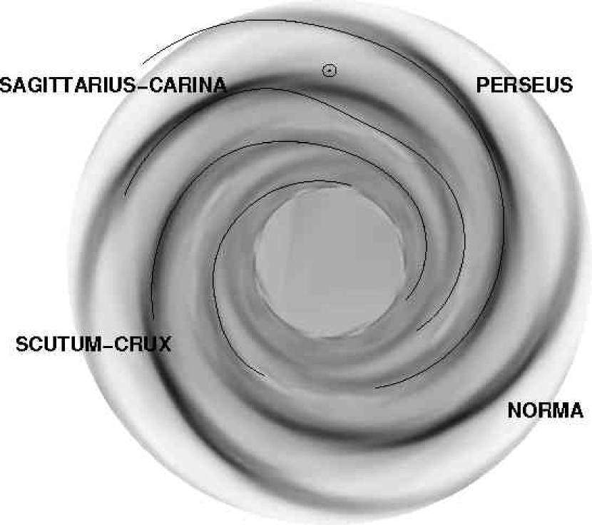
Figure 1.— Surface density of the simulation, compared with the Milky Way’s spiral arms, as traced by Georgelin & Georgelin (1976), modified by Taylor & Cordes (1993). The position chosen for the observer in the following synthetic maps is also presented. The galactocentric distance for the Sun was chosen to be $8\mbox{~{}kpc}$.

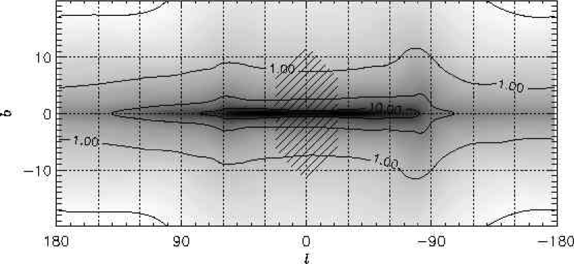
Figure 2.— Column density of the gas, for a region around the galactic plane. The contours are in geometric sequence and labeled in units of $\mbox{~{}kpc}\mbox{~{}cm}^{-3}$. The shaded region marks the inner limit of the simulation domain.

Our position inside the Milky Way Galaxy allows us to make observations at a much higher spatial resolution that we could do in other disk galaxies. But that same fact makes it much more difficult to infer the large scale characteristics of our home galaxy. A lot of the current questions of the spiral structure of the Milky Way could be resolved if we knew the position and full velocity vector of the observed gas. Numerical studies of large scale galactic structure have proved to be very valuable in discerning the sought after characteristics. Nevertheless, this is a very complicated problem and, so far, it is impossible to include all the physics involved. Therefore, modelers must decide which parts of the problem are not going to be considered, in the hope that those neglected will have little influence in the overall conclusions. The models presented here do not include self-gravity of the gas, supernova explosions or other energetic events, and have uncomfortably low spatial resolution. They include a substantial magnetic field, a high thermal pressure (to represent tangled fields, cosmic rays, and subgrid turbulence), and the extra degree of freedom of three dimensions. We believe these are definitive factors that have not been sufficiently explored. The thermal pressure was also adjusted to drop sharply at high densities to encourage the formation of denser structures.

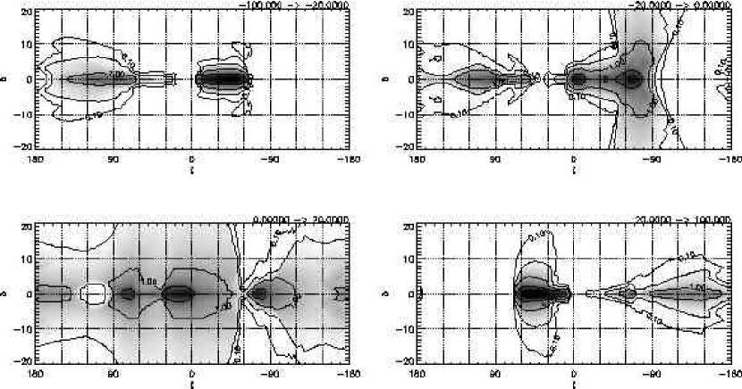
Figure 3.— Same as Figure 2, but restricted in the line-of-sight velocity component of the gas. The range of velocity integration is presented in the top-right corner of each panel, in units of $\mbox{~{}km s}^{-1}$. Most of the higher column density elements in these plots can be traced to spiral arms (or superposition of arms, see text for a discussion). But the one at about $l=75^{\mbox{\small o}}$ in the $0\mbox{~{}km s}^{-1}<v_{los}<20\mbox{~{}km s}^{-1}$ is in an interarm direction, in which the streaming motions generate a small range in line-of-sight velocities over a large path length.

In the first two papers of this series (Gómez & Cox, 2002, 2004, Papers I and II from here on), we presented the results of our simulations of the ISM response to a spiral gravitational perturbation. We showed that the extra stiffness that the magnetic field adds to the gas makes it develop a combination of a shock and a hydraulic jump with significant complications added by vertical bouncing. This jump/shock leans upstream above the plane (more in the two-arm models than the four-arm ones), ahead of the main gas concentration in the midplane. As it shocks, the gas shoots up to higher $z$ in a way similar to water jumping over an obstacle in a riverbed. The gas then accelerates as it runs over the arm, and falls down behind it, generating a secondary set of shocks. In the two-arm cases, the gas bounces back up, generating interarm structures that mimic the ones found at the arms.

In this work, we’ll focus in the four-arm case, designed to have spiral arms similar to those traced by Georgelin & Georgelin (1976), as modified by Taylor & Cordes (1993). In Figure 1 we show the surface density of the four-arm model from Paper II, along with the aforementioned arm pattern, and the corresponding position of the Sun. Notice that the scale of the spiral arms has been reduced so that the distance from the Sun to the galactic center is $8\mbox{~{}kpc}$, as in our model. In Section 2 we present all sky column density maps in radial velocity ranges; in Section 3 we present synthetic longitude-velocity diagrams; in Section 4 we present velocity-latitude diagrams, which we believe have a definite signature of these models; in Section 5 we present the rotation curve that would be measured in this galaxy as affected by the spiral arms; in Section 6 we analyze its effect on the measured kinematic distances in the galactic plane; in Section 7 we examine the rotation of gas above the midplane; in Section 8 we present an all sky synchrotron map; and in Section 9 we present our conclusions.

2. All sky maps.

Figure 2 shows a map of the integrated column density of the simulation, as seen from the position of the observer marked in Figure 1, in galactic coordinates. The grayscale shows the column density, with contours in a geometric sequence and labeling in units of $\mbox{~{}kpc}\mbox{~{}cm}^{-3}$. (The reader should keep in mind that our model spans only from $3\mbox{~{}kpc}$ through $11\mbox{~{}kpc}$ in radius, and up to $1\mbox{~{}kpc}$ in $z$. The shaded region in the galactic center direction shows the angular extent of the central “hole” in our simulation grid. In addition, the full strength of the perturbation is applied only for $r>5\mbox{~{}kpc}$, and therefore, the useful part of the grid extends from $r=5$ to $11\mbox{~{}kpc}$.) Two vertical protuberances are clear in this Figure, corresponding to the directions tangent to the Sagittarius arm, at $l\sim 60^{\mbox{\small o}}$ and $l\sim-75$. Imprints corresponding to other arms are also present; they are harder to pick up in this Figure, but become evident when we restrict the line-of-sight integration to certain velocity ranges, as in Figure 3. (A map with the line-of-sight component of the velocities for the midplane is presented in Figure 4). The Perseus arm appears in all the velocity ranges, but it is more prominent in $l>90^{\mbox{\small o}}$ at negative velocities, and $l<-90^{\mbox{\small o}}$ at $v>20\mbox{~{}km s}^{-1}$. Also prominent are: a superposition of the Perseus, Scutum and Norma arms at between $l\sim 0^{\mbox{\small o}}$ and $-60^{\mbox{\small o}}$ at $v<-20\mbox{~{}km s}^{-1}$; the Sagittarius arm from $l\sim-60^{\mbox{\small o}}$ to $-90^{\mbox{\small o}}$ at intermediate negative velocities, with a very large vertical extension; and a superposition of the Sagittarius and Scutum arms at from $l\sim 0^{\mbox{\small o}}$ to $60^{\mbox{\small o}}$ for large positive velocities.

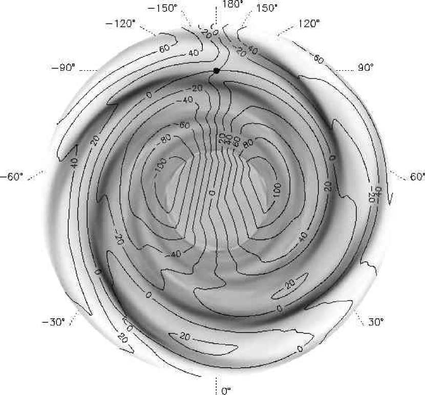
Figure 4.— Surface density of the simulation with the midplane line-of-sight velocities overplotted. The position of the observer is marked by the dot. Galactic longitudes are also labeled.

The diagram for $0<v_{los}<20\mbox{~{}km s}^{-1}$ features three large column density elements. The one at $l\sim-75^{\mbox{\small o}}$ corresponds to the Sagittarius arm. At $l\sim 0^{\mbox{\small o}}$ to $30^{\mbox{\small o}}$, we see a narrow stripe of the whole inner galaxy, including the Perseus, Scutum, and Sagittarius arms. The third element, at $l\sim 75^{\mbox{\small o}}$, corresponds to a tangent direction through the region between the Sagittarius and Perseus arms, in which lower density gas spans a large distance with a small range of velocities.

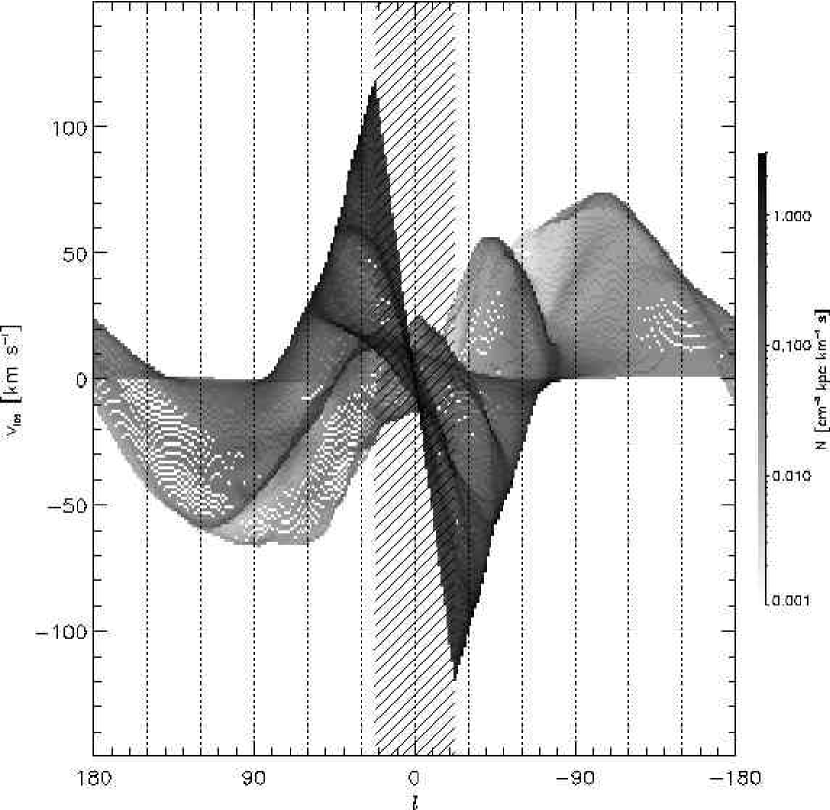
Figure 5.— $l-v$ diagram for $b=0^{\mbox{\small o}}$. The shaded region marks the “hole” in our simulation grid. Many features of the observed $l-v$ diagrams are reproduced: the asymmetry in the inner rotation curve, the non-zero mean velocity in the $l=180^{\mbox{\small o}}$ direction, and the high column density ridges, usually associated with spiral arms.

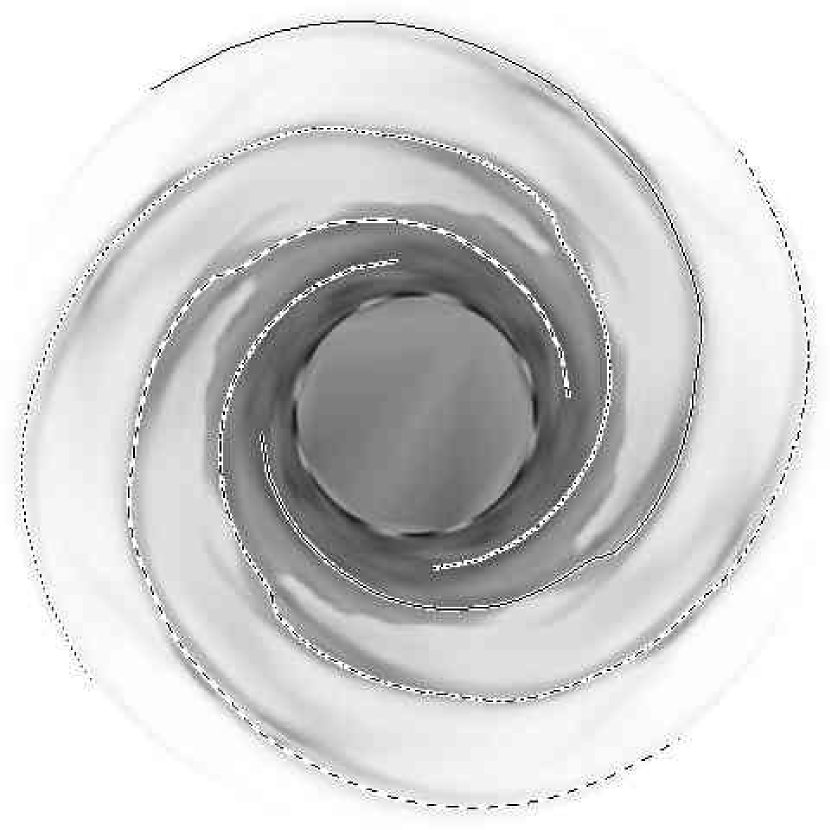
Figure 6.— Loci of the spiral arms traced by fitting a sinusoidal function to the vertical column density, for each radius. The solid line traces the Perseus arm, dashed-dotted the Norma arm, dashed the Scutum, and dotted the Sagittarius arm. The grayscale is the midplane density of the model.

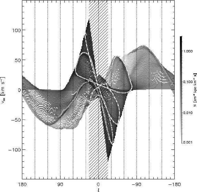
Figure 7.— Same as in Figure 5, with the spiral arms from Figure 6 traced on it. The solid line traces the Perseus arm, dashed-dotted the Norma arm, dashed the Scutum, and dotted the Sagittarius arm. Notice that not all the ridges correspond to arms, and not all the arms trace back to ridges.

3. $l-v$ diagram.

Longitude-velocity diagrams are a straightforward way of presenting the data-cubes, and it is relatively easy to extract information about global properties of the Galaxy. Figure 5 shows a longitude-velocity diagram, as seen by an observer situated as marked in Figure 1, at galactic latitude $b=0^{\mbox{\small o}}$. Again, the shaded region marks the region around the galactic center that we do not include in our model. Several features can be pointed out. The rotation curve, as traced by the extremum velocity of the gas in the inner galaxy, has small deviations from a flat curve which are not symmetric about $l=0^{\mbox{\small o}}$ (see Section 6). Even without velocity dispersion intrinsic to the gas in the model, there is a fair amount of gas moving at forbidden velocities in the general direction of the galactic anticenter (positive in the second quadrant, negative in the third). Also, the gas in the anti-center direction has a positive mean velocity, while the envelope of the emission averages to zero at $l\sim 170^{\mbox{\small o}}$. These characteristics depend strongly on the chosen position for the observer. Features similar to these are observed in $l-v$ diagrams from Milky Way’s H I surveys, although details (like the longitude of the zero velocity around the anticenter) do not necessarily coincide with our model. The proximity of our outer boundary ($3\mbox{~{}kpc}$ in the anticenter direction) might have some influence on this.

Ridges and intensity enhancements in this diagram are usually interpreted as spiral arms. Since in our model we have the advantage of knowing exactly where the material is and with which velocity it is moving, we can trace the gaseous spiral arms into the simulated $l-v$ diagram. We found the position of the spiral arms by fitting, for each radius in the simulation grid, a sinusoidal function along azimuth to the vertical column density of the gas. Figure 6 presents the result of the fit, while Figure 7 traces the spiral arms into the $l-v$ diagram. Most of the ridges in this diagram correspond to spiral arms, although the relation is not one-to-one. For example, around $l=120^{\mbox{\small o}}$, at the Perseus arm, the line of sight goes through a large velocity gradient, which spreads the arm in velocity, and diffuses the ridge. The converse also happens: lower intensity ridges that are not related to spiral arms are generated when the velocity gradient is small, and large spatial extents condense into a small velocity range, for example, at $(l,v)\sim(-90^{\mbox{\small o}},30\mbox{~{}km s}^{-1})$. The capacity of the velocity field to create or destroy structures in this diagram with little regard of the underlying gas density has been long known (Burton, 1971; Mulder & Liem, 1986).

4. $v-b$ diagram.

Another natural way of presenting data cubes is the velocity-latitude diagram. For our model, the $v-b$ diagram shows the signature of the vertical structure of the spiral arms.

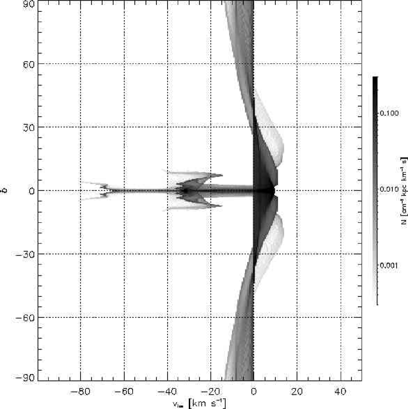
Figure 8.— $v-b$ diagram along $l=75^{\mbox{\small o}}$. Notice the gas at negative velocities around the galactic pole directions and the vertical ridge at $v\sim-10\mbox{~{}km s}^{-1}$ above $b\sim 50^{\mbox{\small o}}$, created by velocity crowding. The structure is truncated for $v<-70\mbox{~{}km s}^{-1}$ by encounter with the edge of the simulation grid.

Figure 8 shows the $v-b$ diagram for the $l=75^{\mbox{\small o}}$ direction. The position chosen for the observer places it just downstream from the Sagittarius arm, where the gas is falling down. Therefore, Figure 8 shows gas with negative velocities at large galactic latitudes. This is consistent with the observations by Dieter (1964), the WHAM project (Haffner et al., 2003), and other authors, which found that gas around the galactic poles has a mean negative velocity. Notice the higher intensity ridge that runs from $v=0\mbox{~{}km s}^{-1}$ at $b\sim 40^{\mbox{\small o}}$ to about $v=-8\mbox{~{}km s}^{-1}$ at the galactic pole. That ridge is generated by crowding of the falling gas in velocity space. A spectrum taken toward those latitudes would show a line that could be interpreted as a cloud, although the gas has no spatial concentration.

Figure 9 zooms into a $20^{\mbox{\small o}}$ region around the galactic midplane. Examination of Figure 4 shows that such line-of-sight crosses the Perseus arm at $v\sim-30\mbox{~{}km s}^{-1}$ and the Norma arm at $v\sim-70\mbox{~{}km s}^{-1}$, very close to the simulation edge. At those approximate velocities, Figures 8 and 9, show “mushroom” shaped structures, with a relatively narrow, horizontal stem and large vertical cap on the left edge of the stem. These are the characteristic signatures of the vertical structure of the gaseous arms, along with a tendency of the tip of the cap to bend slightly back over the stem, to less negative velocities at higher latitude.

In order to guide the following discussion, we present in Figure 10 the density (grayscale) and line-of-sight component of the velocity (contours) along a vertical plane in the $l=75^{\mbox{\small o}}$ direction. Since we are looking at the arm from the concave side, the gas moves through it from left to right, though not parallel to the plane of the Figure. The reader should keep in mind that these velocities are the result of the presence of the arms on top of the galactic rotation. If the gas were in purely circular orbits, we should see positive velocities up to the solar circle, at a distance of $4.1\mbox{~{}kpc}$, and then negative velocities, monotonically decreasing until the edge of the grid. This general pattern is found in the Figure, with velocities increasing from 0 to $+10\mbox{~{}km s}^{-1}$ at $\sim 2\mbox{~{}kpc}$, then back to zero at $\sim 4\mbox{~{}kpc}$, going increasingly negative, though not monotonically, beyond that.

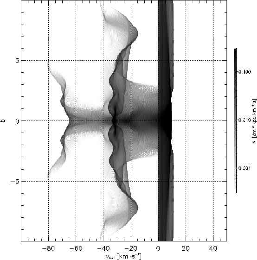
Figure 9.— Same as Figure 8, zooming to $20^{\mbox{\small o}}$ around the galactic plane. The horizontal mushroom shapes are consequences of the three dimensional structure of the spiral arms, as discussed in the text. For this longitude, the structure at $v\sim-30\mbox{~{}km s}^{-1}$ corresponds to the Perseus arm, and the structure at $v\sim-70\mbox{~{}km s}^{-1}$ corresponds to the Norma arm. See also Figure 10.

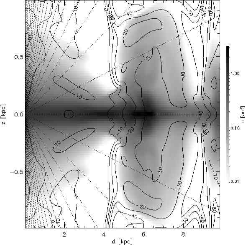
Figure 10.— Logarithm of density (grayscale) and line-of-sight component of the velocity (contours) along the $l=75^{\mbox{\small o}}$ direction. The velocity contours are labeled in $\mbox{~{}km s}^{-1}$ units. The dotted lines mark the latitude directions every $5^{\mbox{\small o}}$. The abscissa is the distance from the position of the observer. As the gas falls from the Sagittarius arm, it compresses the disk before flowing into the Perseus arm (at $d\sim 6\mbox{~{}kpc}$), where it is slowed down and forms the narrow stem of the “mushroom” structure in Figure 9. The gas swells around the spiral arm, and the high latitude flow speeds up as it passes over the midplane lump. This flow shows in Figure 9 as the tips of the mushroom cap bent toward less negative velocities. After the arm, the gas falls into the midplane, compressing the disk before the flow shocks into the Norma arm (near the outer boundary).

Let us concentrate on the Perseus arm, at about $6\mbox{~{}kpc}$. Just upstream from the arm, there is a vertically thin distribution of material formed by the downflow from the Sagittarius arm. The encounter of this material with the arm decelerates the gas, appearing as a rapid succession of decreasing velocity contours at $d\sim 4.5\mbox{~{}kpc}$. That velocity gradient spreads the vertically thin gas structure along the horizontal axis of the $v-b$ diagram, creating the stem structure in the midplane. Beyond $\sim 5\mbox{~{}kpc}$, we have the vertically swelled structure of the arm itself, which appears in Figure 9 as the vertically extended mushroom cap. Between $b\sim 5^{\mbox{\small o}}$ and $7^{\mbox{\small o}}$, the gas is speeding up above the arm increasing its line-of-sight velocity, causing the tip of the cap to slightly bend back over the stem. (The reversal of this trend between $b\sim 7.5^{\mbox{\small o}}$ and $10^{\mbox{\small o}}$ involves a very small amount of material very close to the vertical boundary and could be an artifact.) Within the arm, the radial velocity has one or more extremes, creating caustics as the gas doubles back in velocity space. This behavior repeats as we approach the Norma arm, but we reach the simulation boundary before developing the full arm structure, and we get only the stem and the beginning of the cap.

When we restricted the integration to the thin preshock interarm region, we noticed that its $v-b$ imprint is very small. But, as seen in Figure 10, the true “interarm” region is much broader and includes the high $z$ part of the cap of the previous arm, after the midplane density has decreased.

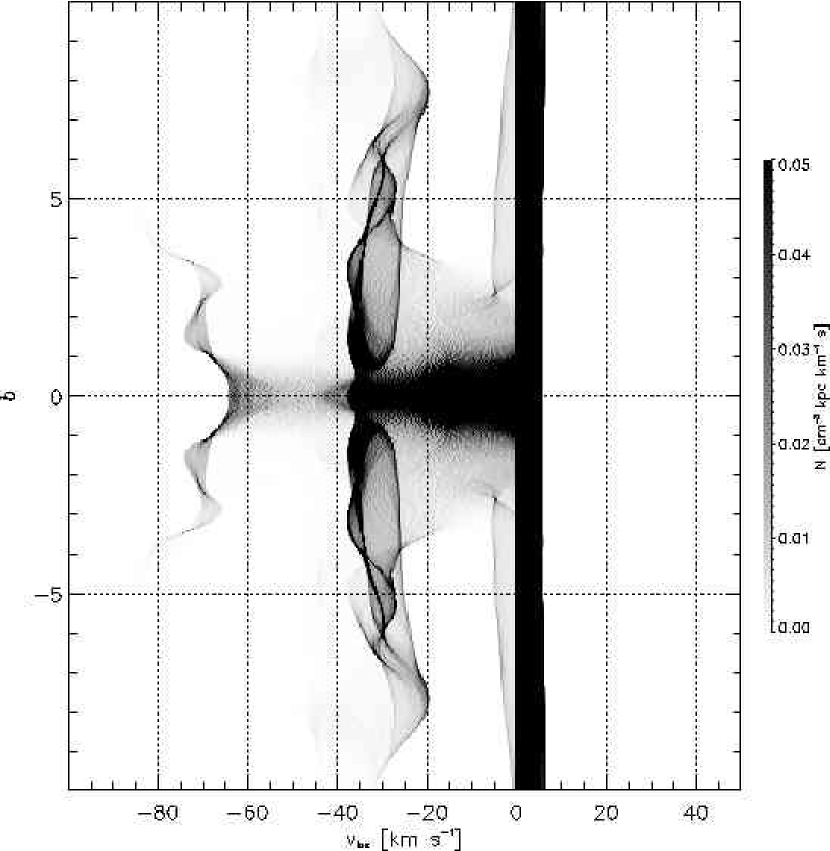
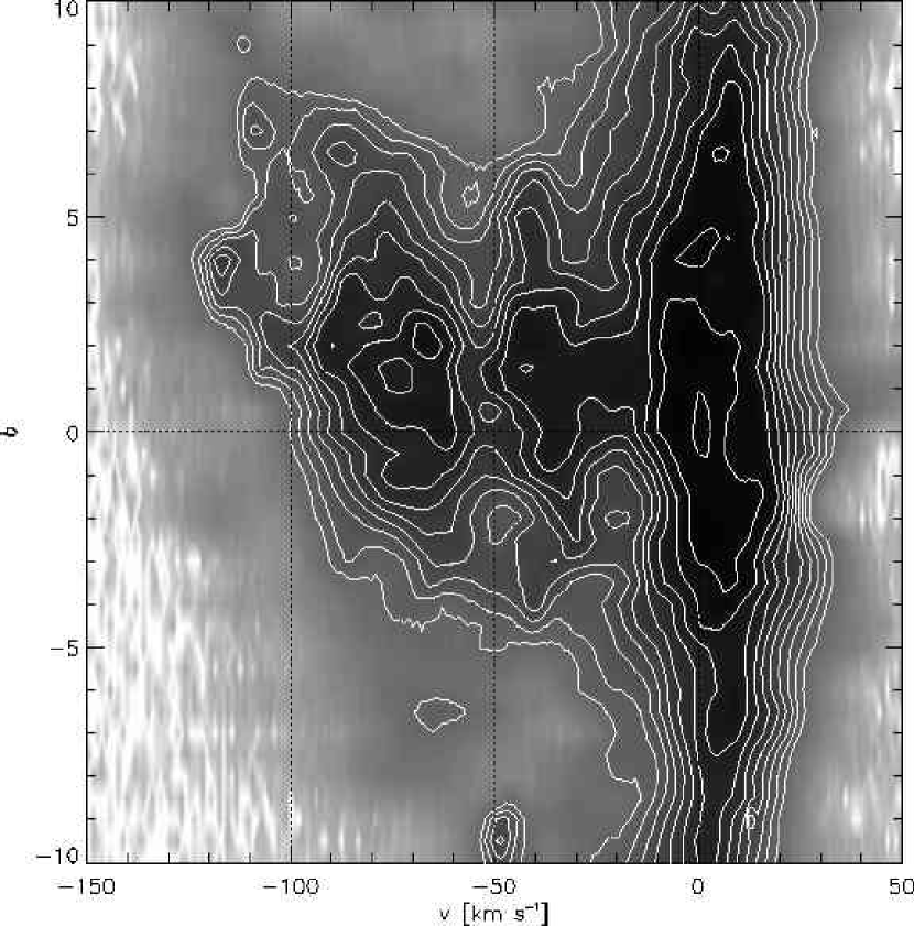
Figure 11.— $v-b$ diagrams for $l=79^{\mbox{\small o}}$ for the simulation and the Leiden/Dwingeloo survey. The grayscale presents the column density at a given velocity (arbitrary units for the survey) in a linear scale. Notice that the galactic warp is present in the survey data, while the symmetry in the simulation does not allow a warped disk. Once again, the encounter with the edge of the calculation grid truncates the model distribution for $v<-70\mbox{~{}km s}^{-1}$. Note that, in both the model and the data, the stem structure of the Norma arm (between $-40$ and $-65\mbox{~{}km s}^{-1}$) is much less pronounced than that of the Perseus arm (between $0$ and $-35\mbox{~{}km s}^{-1}$). Its existence relies on the production of a thin dense region ahead of the arm by the interarm downflow. As seen in Figure 10, at $d\sim 8.5\mbox{~{}kpc}$, this region is thin, but not so dense as that ahead of the Perseus arm.

In Figure 11, the $v-b$ diagram for the simulation in the $l=79^{\mbox{\small o}}$ direction is compared with the equivalent diagram for the Leiden/Dwingeloo H I survey (Hartmann & Burton, 1997). The now familiar mushroom structures appear again at the approximate velocities of the spiral arms, along with the characteristic gap between caps of successive arms. At other galactic longitudes, the observed pattern is less regular, presumably due to galactic complexities not found in our model. Notice that, in the survey data, the galactic warp displaces the mushroom structures off the $b=0^{\mbox{\small o}}$ plane, while restrictions in the simulation does not allow such symmetry break.

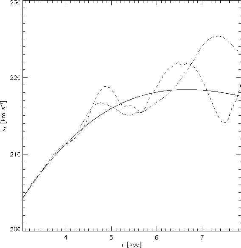
Figure 12.— Rotation curve for the midplane derived by simulating measurements in the model. The continuous line is the rotation law in the setup, the dotted line is the derived rotation for positive longitudes, and the dashed line is for negative longitudes. Our “measured” rotation curve is larger in the $6.8\mbox{~{}kpc}<r<8\mbox{~{}kpc}$ range for positive longitudes than for negative longitudes. The opposite is true for the $4.3\mbox{~{}kpc}<r<6.8\mbox{~{}kpc}$ range. Both trends approximate features of the measured rotation curves of the Milky Way discussed in the text.

5. Rotation curve.

In order to estimate the influence of the spiral arms on measurements of the galactic rotation curve, we measured it in the simulation in a way that emulates how it is measured in the Milky Way. For gas inside the solar circle, we picked a galactic longitude. We then looked for the maximum velocity along the line-of-sight (minimum for negative longitudes) and assumed that it arises from the tangent point and, therefore, the gas at that galactocentric radius moves with that extreme velocity. By repeating this procedure for an array of galactic longitudes, we can trace the rotation curve interior to the solar circle. Figure 12 shows the results. The dotted line shows the case for the northern galaxy, while the dashed line shows the rotation curve for the southern galaxy. For comparison, the rotation curve that arises from the hydrostatic plus rotational equilibrium in the initial conditions is presented as the continuous line.

The observed rotation curve (Blitz & Spergel, 1991; McClure-Griffiths et al., 2004, when scaled for $r_{\odot}=8.0\mbox{~{}kpc}$) is systematically higher in the range $55^{\mbox{\small o}}<l<80^{\mbox{\small o}}$ ($6.5\mbox{~{}kpc}<r<7.8\mbox{~{}kpc}$) than in the corresponding negative longitudes by some $7\mbox{~{}km s}^{-1}$. The converse happens in the $40^{\mbox{\small o}}<l<55^{\mbox{\small o}}$ range ($5\mbox{~{}kpc}<r<6.5\mbox{~{}kpc}$). This behavior and the amplitude of the oscillations are reproduced by our simulations, although around $r=7.5\mbox{~{}kpc}$, the difference between our rotation curves, $\sim 10\mbox{~{}km s}^{-1}$, is somewhat larger than observed.

6. Kinematic distances.

An important use of the rotation curve is the estimation of distances in the Galaxy, by assuming that the target moves in a circular orbit. In this section we try to estimate the error in those distances. The fact that the calculated curve falls below the rotation set by the rotational hydrostatics and the background potential (Figure 12) creates lines of sight in which the gas never reaches the velocity that direction should have in circular orbit, and therefore, if this “true rotation” is used to estimate distances, no gas would be assigned to those regions. If we imagine the galaxy as made of rubber and being distorted by the distance errors, the picture obtained would have large holes in those regions. For this reason, and for self-consistency, we used the rotation curve derived in Section 5.

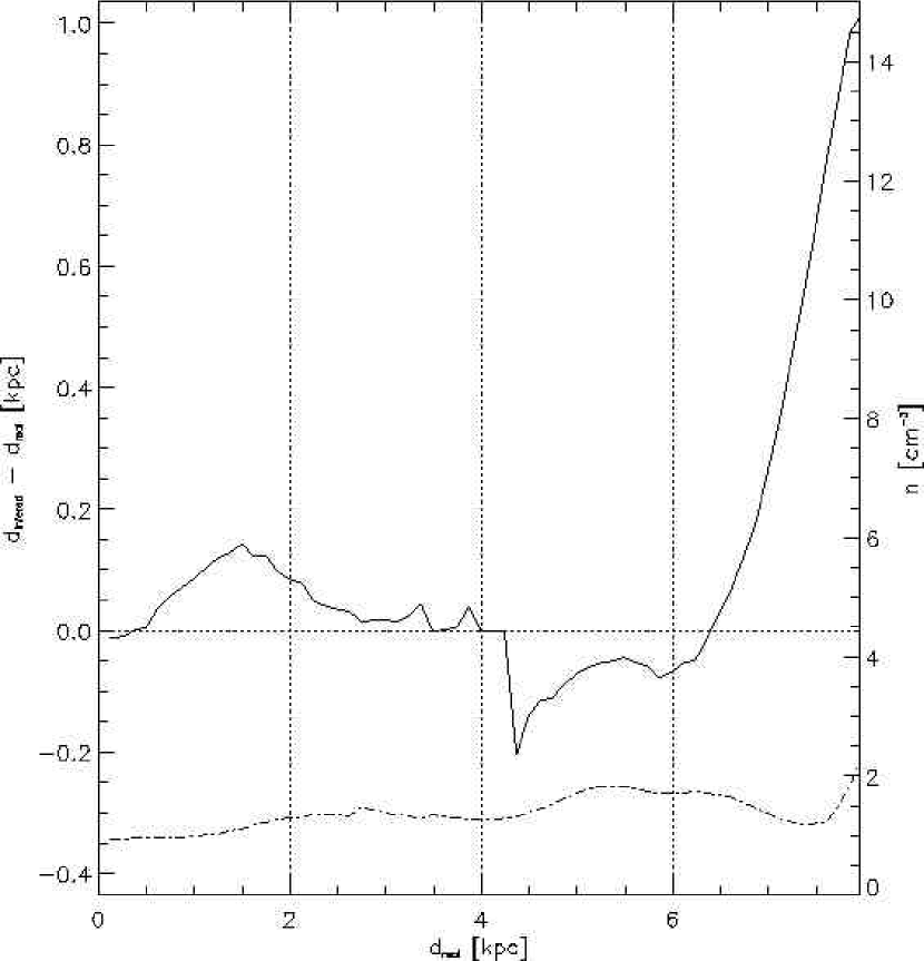
Figure 13.— Error in the estimated distance due to the assumption of circular orbits, along the $l=60^{\mbox{\small o}}$ direction. Our “measured” rotation curve from Figure 12 was used to obtain the kinematic distances. The dashed-dotted line is the gas density at that (real) distance. Generally speaking, the distance is overestimated at the arms, and underestimated in the interarms, although this depends on the chosen galactic longitude.

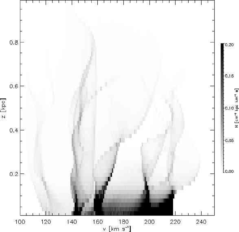
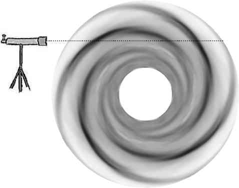
Figure 14.— The left panel shows the spectrum that an observer would get when placing the slit perpendicular to the galactic plane, at a distance of $6.2\mbox{~{}kpc}$ from the center. The grayscale shows the column density for a given velocity above the galactic plane. As shown in the right panel, the line of sight crosses three spiral arms, respectively from left to right, at $160,195$ and $145\mbox{~{}km s}^{-1}$. The fourth midplane concentration, between 200 and $218\mbox{~{}km s}^{-1}$ is along the tangent line, in an interarm region.

Since we have the privileged information of where the gas really is, we can estimate the error created by assuming that the gas moves in circular orbits with the adopted rotation curve. At a given distance along a fixed longitude direction, we take the velocity of the gas given by the simulation, and calculate at what distance the circular orbit assumption puts it. Even if the rotation curve has oscillations, the line-of-sight velocity of the gas in circular orbits might remain monotonic on either side of the tangent point, provided that the oscillations are not too large (as can be seen in Figure 10, that is not the case above the plane, but here we focus in the distances along the midplane). Therefore, there is still only a two-point ambiguity in the assigned distance. We solve that ambiguity by cheating: we place the gas parcel on the side of the tangent point we know it to be.

Figure 13 shows the error in the estimated distance along the $l=60^{\mbox{\small o}}$ direction. In order to compare these errors to the spiral arms, the density is plotted also (dashed-dotted line). Although it depends on the galactic longitude, the distances tend to be over-estimated around the arms and under-estimated in the interarms by a varying amount, typically smaller than $1\mbox{~{}kpc}$. Gas moving at forbidden velocities cannot be given a location with this method.

7. Cylindrical rotation.

Kinematics of the gas above the galactic plane has been studied as a test for models for the galactic fountain, which in turn are used to explain the ionization of the ISM at high $z$ (see discussion in Miller & Veilleux 2003). Unfortunately, the velocity resolution achieved for external galaxies makes it difficult to estimate rotation velocity gradients over the vertical distance our models span, and therefore comparison is difficult. Nevertheless, we present in Figure 14 a synthetic spectrum that could be obtained by placing the slit perpendicular to the galactic plane, at a distance of $6.2\mbox{~{}kpc}$ from the galactic center. Three spiral arm crossings are clear in this picture, at $160,195$ and $145\mbox{~{}km s}^{-1}$ (respectively, as we move away from the observer). Notice that the arms show a leaning toward higher velocity as we move up, due to the gas speeding up over them after the shock. Also, the arm at $195\mbox{~{}km s}^{-1}$ spreads over a range of velocities, since we look at it at a smaller angle.

The right limit of the emission in this diagram is usually associated with the rotation of the galaxy. That maximum velocity is not reached at the point of smallest radius, the tangent point, but the offset is quite small ($1\mbox{~{}kpc}$ or less). That point corresponds to an interarm region, where the gas falls back down to the plane, and slows down as it moves out in radius. Therefore, near the midplane, this maximum velocity falls below the rotational velocity that we get when repeating this exercise at a different radius.

As in previous cases, not all the ridges in this plot correspond to density structures, but are generated by velocity crowding. Such is the case of the element at $v_{los}>220\mbox{~{}km s}^{-1}$ around $z=200\mbox{~{}pc}$, which is generated by a plateau of nearly constant velocity in a region with density lower than its surroundings, which have a larger spread in velocity.

From Figure 14, we would infer that the velocity maximum increases some $20\mbox{~{}km s}^{-1}$ up to $z=200\mbox{~{}pc}$, and then comes back down to $220\mbox{~{}km s}^{-1}$ around $z=400\mbox{~{}pc}$. When placing the slit at a different position, we get similar behavior, with different amplitudes and at different heights. Miller & Veilleux (2003) observed a similar behavior in a couple of galaxies in their sample, although with a larger velocity amplitude. Those seem to be exceptions, since most of the galaxies in their sample do not show significant gradients. The amplitude of the velocity gradient in this model would have been difficult to detect with the resolution achieved in their study.

8. Synchrotron emission.

Figure 15 shows an all sky map of the synchrotron emission. The grayscale corresponds to the total synchrotron intensity, while the direction of the magnetic field, as inferred from the polarization of the integrated emission, is presented in dashes. The synchrotron emissivity is given by

$$\varepsilon_{tot}(r,\phi)\propto n_{cr}(r,z)B_{\perp}^{(p+1)/2},$$ (1)

where $B_{\perp}$ is the component of the magnetic field perpendicular to the line-of-sight, $p=2.5$ is the spectral index of the distribution of cosmic ray electrons, $n_{cr}=\exp(-r/r_{cr}-z/z_{cr})$ is its space density, $r_{cr}=13\mbox{~{}kpc}$ and $z_{cr}=2.5\mbox{~{}kpc}$ (Ferrière, 1998). For each $(l,b)$ direction, this emissivity is integrated, and the direction of the polarization is accounted for by the process described in Paper II.

The degree of polarization of the integrated emission is generally high, varying from $>70\%$ in the midplane and in the $l\sim 0^{\mbox{\small o}}$ and $180^{\mbox{\small o}}$ at all latitudes, to $\sim 40\%$ in four isolated regions toward $(l,b)\sim(\pm 120^{\mbox{\small o}},\pm 70^{\mbox{\small o}})$. This is expected, since our resolution does not allow us to model the random component of the field.

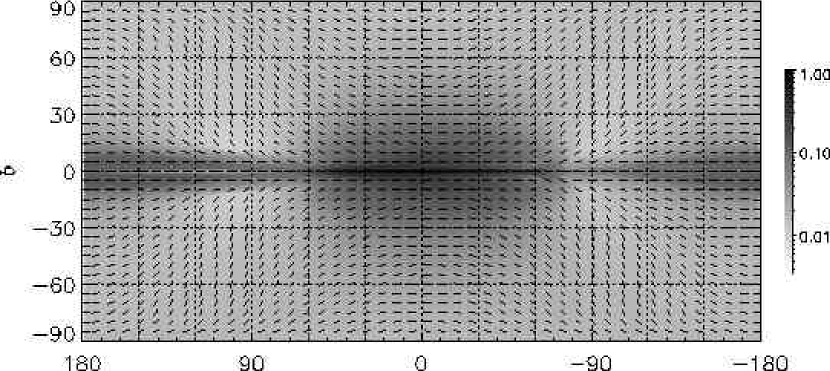
Figure 15.— All sky map of synchrotron emission, in arbitrary units. The dashes mark the direction of the magnetic field, as implied from the polarized emission. With exception of the midplane, a circular field pattern is observed, although the field in the simulation is not.

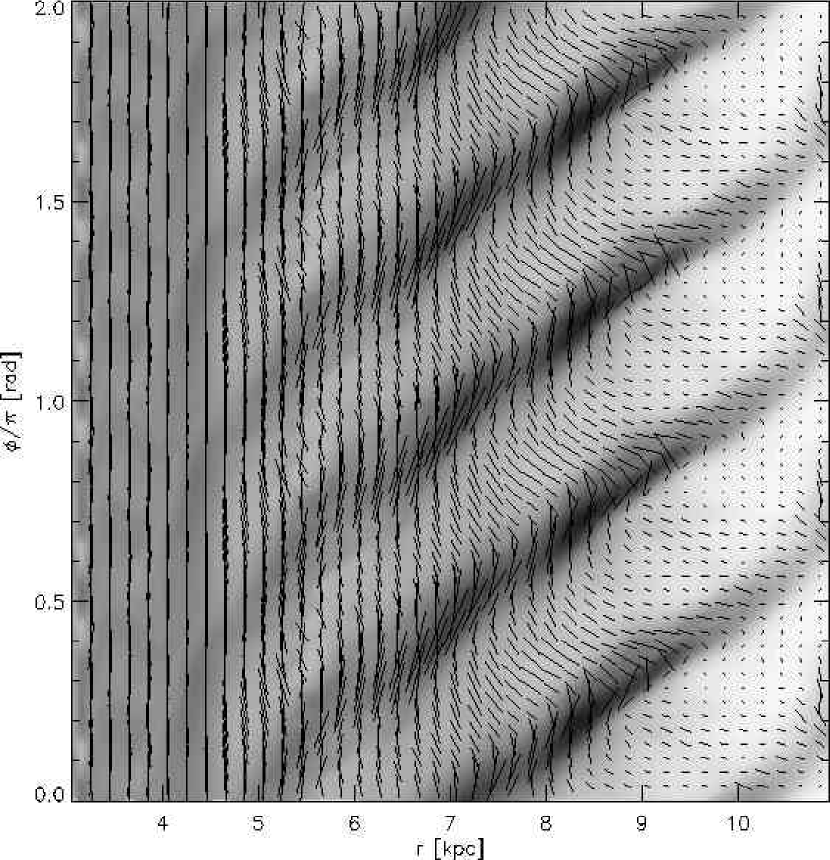
Figure 16.— Reproduced from Paper II, this Figure presents the direction of the magnetic field in the midplane, displayed in a polar diagram. The axes show the radius from the galactic center and the azimuthal angle (the Sun would be in the $(r,\phi)=(8\mbox{~{}kpc},\pi/2)$ position). The orbiting gas flows down from the top. The length of the dashes is proportional to the field strength. The grayscale represents the surface density of the simulation. Notice that the field adopts a negative pitch angle in the interarm region.

To help with the discussion of this map, we present the midplane magnetic field in the simulation in Figure 16, reproduced from Paper II. The grayscale represents the surface density, and the dashes follow the direction of the magnetic field, with its length proportional to the field strength.

Recalling Figure 1, the second and third quadrants have interarm gas nearby. The Perseus arm is $2\mbox{~{}kpc}$ away in the $l=180^{\mbox{\small o}}$ direction, and $5\mbox{~{}kpc}$ away toward $l=90^{\mbox{\small o}}$. In that $90^{\mbox{\small o}}<l<180^{\mbox{\small o}}$ range, near the midplane, the magnetic field has a negative pitch angle. This has the effect that the field is pointing directly toward the observer, and the plane-of-the-sky component is very small, causing the low emission at low latitudes in Figure 15. Around the $l=-90^{\mbox{\small o}}$ direction, that negative pitch angle increases the component of the field projected in the sky, causing a higher emission in the $-90^{\mbox{\small o}}<l<-60^{\mbox{\small o}}$ range. On the other hand, the field above the plane twists more abruptly, with a smaller negative pitch region, yielding a short path length to integrate over and leaving only a small imprint on this plot. As a consequence, off the galactic plane, we see a pattern in the sky that resembles that of a circular field: horizontal in the $l\sim 0^{\mbox{\small o}}$ and $180^{\mbox{\small o}}$ at all latitudes, and in the midplane, at all longitudes; nearly vertical off the plane in the $l\sim 90^{\mbox{\small o}}$ and $-90^{\mbox{\small o}}$ directions (the sky projection of an overhead circle).

Although the sign of the radial component of the field changes between the arm and interarm regions, those changes are not enough to account for the changes in the differential rotation measure that are typically interpreted as reversals in the direction of the galactic magnetic field (Beck, 2001, and references therein).

9. Conclusions.

By placing an imaginary observer inside the modeled galaxy from Paper II, we generated various synthetic observations. Since we actually know where the gas is, we can distinguish which parts of the model are generating the observed structures. In particular, velocity crowding effects can be distinguished from real spatial concentrations.

The synthetic $l-v$ diagram has common characteristics with the observed diagram, although some similarities are only in a qualitative level. Again, velocity crowding generates ridges that do not correspond to spiral arms. But the converse also happens, as a large velocity gradient can dilute a spiral arm in velocity space. In the $v-b$ diagram, on the other hand, velocity crowding and dilution generate structures that test the vertical distribution of matter and velocity above the arms presented in Papers I and II. Such structures can be observed in the Leiden/Dwingeloo H I survey.

We also explored the rotation curve that the imaginary observer would measure from within the model galaxy. Several of the characteristics of this measured rotation curve are also observed in the curve measured for the Milky Way, being higher in some radial ranges than on the opposite side of the galactic center. This agreement is probably a consequence of our having tried to fit the positions of the spiral arms in our model to the proposed positions for the Galaxy. Nevertheless, the measured rotation curve has large deviations with respect to the rotation from our initial conditions, which is also influenced by pressure gradients and magnetic tension and is therefore slightly different from the rotation consistent with the background gravitational potential.

Although the magnetic field is largely non-circular, the averaging effect of the synthetic synchrotron maps generates a largely circular imprint, with exception of the midplane. As mentioned in Paper II, restrictions in our model limit the amount of vertical field that our model generates, increasing the circularity of the field and diminishing the vertical extent of the synchrotron emission.

The ISM of the Milky Way Galaxy is very complex system, in which many different physical processes combine to generate large scale structure. The extra freedom of the third dimension and the dynamical effects of a strong magnetic field, in our view, are two key elements in the formation of such structures. Until we find a way of reliably measuring distances to the diffuse components of the disk, velocity crowding effects will keep blurring and distorting the pictures we generate. More realistic modeling with higher resolution, inclusion of gas self-gravity, and stellar feedback (including cosmic ray generation and diffusion) is necessary to further clarify that picture.

References

- Beck (2001) Beck, R. 2001, Space Sci. Rev., 99, 243
- Blitz & Spergel (1991) Blitz, L. and Spergel, D. N. 1991, ApJ, 370, 205
- Burton (1971) Burton, W. B. 1971, A&A, 10, 76
- Dieter (1964) Dieter, N. H. 1964, AJ, 69, 137
- Ferrière (1998) Ferrière, K. 1998, ApJ, 497, 759
- Georgelin & Georgelin (1976) Georgelin, Y. M. and Georgelin, Y. P. 1976, A&A, 49, 57
- Gómez & Cox (2002) Gómez, G. C. and Cox, D. P. 2002, ApJ, 580, 235 (Paper I)
- Gómez & Cox (2004) Gómez, G. C. and Cox, D. P. 2004, ApJ, submitted (Paper II)
- Haffner et al. (2003) Haffner, L. M., Reynolds, R. J., Tufte, S. L., Madsen, G. J., Jaehnig, K. P. and Percival, J. W. 2003, ApJS, 149, 405
- Hartmann & Burton (1997) Hartmann, D. and Burton, W. B. 1997, Atlas of Galactic Neutral Hydrogen (Cambridge: Cambridge Univ. Press)
- McClure-Griffiths et al. (2004) McClure-Griffiths, N. M., Dickey, J. M., Gaensler, B. M. and Green, A. J. 2004, ApJ, submitted
- Miller & Veilleux (2003) Miller, S. T. and Veilleux, S. 2003, ApJ, 592, 79
- Mulder & Liem (1986) Mulder, W. A. and Liem, B. T. 1986, A&A, 157, 148
- Taylor & Cordes (1993) Taylor, J. H. and Cordes, J. M. 1993, ApJ, 411, 674