3D MHD Modeling of the Gaseous Structure of the Galaxy: Description of the Simulations.

Abstract

As discussed in Gómez & Cox (2002), the extra stiffness that the magnetic field adds to the ISM changes the way it reacts to the presence of a spiral perturbation. At intermediate to high $z$, the gas shoots up before the arm, flows over, and falls behind it, as it approaches the next arm. This generates a multicell circulation pattern, within each of which the net radial mass flux is positive near the midplane and negative at higher $z$. The flow distorts the magnetic field lines. In the arm region, the gas flows nearly parallel to the arm, and therefore, the magnetic field adopts a similar pitch angle. Between the arms, the gas flows out in radius, generating a negative pitch angle in the magnetic field. The intensity and direction of the field yield synthetic synchrotron maps that reproduce some features of the synchrotron maps of external galaxies, like the islands of emission and the displacement between the gaseous and synchrotron arms. When comparing the magnitude of the field with the local gas density, two distinctive relations appear, depending on whether the magnetic pressure is dominant.

Above the plane, the density structure develops a shape resembling a breaking wave. This structure collapses and rises again with a period of about $60\mbox{~{}Myr}$, similar to that of a vertical oscillation mode. The falling gas plays an important part in the overall hydrostatics, since its deceleration compresses the low $z$ gas, raising the average midplane pressure in the interarm region above that provided by the weight of the material above.

1. Introduction.

Spiral structure is an astounding characteristic of disk galaxies. Yet, the nature of the spiral structure of our home galaxy is far from well understood. The generally accepted model, originally discussed by Lindblad (1960), Lindblad (1961) and Lin & Shu (1964), involves a density wave resulting from a global gravitational mode, triggered either by a internal instability or some driving element (like a bar or an interacting external galaxy). Another proposed model describes the spiral structure as a self-propagating wave of enhanced star formation (Mueller & Arnett, 1976). In either case, the models show the importance of the gaseous disk in the global spiral structure phenomenon.

The role of the gas in the spiral structure has been exploited repeatedly in order to trace the spiral arms, both in the Milky Way and in external galaxies. Those efforts have included H I (Oort, Kerr & Westerhout, 1958), CO clouds (Dame et al., 1986) and dust (Drimmel, 2000) as tracers. Since the spiral arms show an enhanced star formation rate, Pop I objects can also be used as tracers. The model presented by Georgelin & Georgelin (1976), which featured a four-arm spiral traced by galactic H II regions, is frequently cited. Nevertheless, it is not unusual to observe differences in the spiral structure when different tracers are used. One example is NGC 2997, in which one clearly defined arm in optical light is absent in infrared light (Block et al., 1994). In the Milky Way Galaxy, Drimmel (2000) found that the dust emission is better fit by a four-arm spiral, while a two-arm spiral fits the stellar emission (Vallée, 2002, presents a review).

As a result of the coupling between the gaseous disk and the interstellar magnetic field, the latter also is influenced by (and influences) the spiral pattern. Since the magnetic fields are “illuminated” by the cosmic rays spinning along the field lines, the so generated synchrotron emission is a direct probe of the field. In external galaxies, the total (polarized + unpolarized) synchrotron emission tends to follow the spiral pattern, although a displacement between the positions at which the optical and synchrotron emission peaks is not unusual. In addition, analysis of the polarization direction of the synchrotron emission shows that the magnetic field is usually aligned with the spiral arms (Beck et al., 1996, 2002). Then, it can be argued that the large scale magnetic field plays a significant role in the formation of spiral structures in disk galaxies.

Martos & Cox (1998) explored what effect a strong galactic magnetic field would have in the vertical structure of the spiral arms. The main difference between their models and previous work was the inclusion of a thicker, higher pressure ISM. The necessity of such environment was pointed out by the fact that some components of the gaseous disk were observed to have scale heights of the order of kpc (Reynolds, 1989; Edgar & Savage, 1989), much larger than those previously considered. The support necessary for the weight of that gas is larger than the thermal pressure observed in the midplane, leading to the conclusion that non-thermal pressures must dominate the vertical hydrostatics of the galactic disk, and that the pressure scale height might be much larger that the density scale height (Boulares & Cox, 1990). When those pressures significantly increase the effective $\gamma$ of the medium, the gas flowing into the spiral arms shows a combination of a shock and a hydraulic jump at the position of the spiral arms, which induced large vertical gas motions. Such behavior appears to have been observed in NGC 5427 (Alfaro et al., 2001).

In an earlier work (Gómez & Cox, 2002, Paper I from here on), we extended Martos & Cox (1998) analysis to three dimensions and included a large fraction of the galactic disk. It is the purpose of this work to further explore those results and aim more directly at the Milky Way structure. The paper is organized as follows: Section 2 summarizes the results of Paper I, presents the initialization of the simulations we present here, and describes the basic features of the flows at an age of $800\mbox{~{}Myr}$; Section 3 describes the magnetic field structure, the synchrotron emission, and the field-density relationships; Section 4 explores the elements of the support of the disk and the vertical hydrostatics near the solar circle; Section 5 explores periodicity and normal frequencies in the simulation; Section 6 describes the large scale motions encountered in the simulation and evidence for circulation; and Section 7 presents our conclusions.

2. The simulation setup.

Details of the setup are provided in Paper I. Here we present only an overview, mentioning the differences from the cases presented there.

We performed three-dimensional MHD simulations using the code ZEUS (Stone & Norman, 1992a, b; Stone, Mihalas & Norman, 1992) to model the ISM response to a spiral gravitational perturbation. The gas starts in vertical and radial hydrostatic equilibrium, following the circular orbits defined by the background gravitational potential from model 2 in Dehnen & Binney (1998), the pressure gradient (thermal plus magnetic), and the magnetic tension. The magnetic field is azimuthal, with a strength defined by the relation:

$$p_{B}=p_{M}\frac{n}{n+n_{c}}\mbox{~{}dyn}\mbox{~{}cm}^{-2},$$ (1)

where $p_{B}$ is the magnetic pressure, $p_{M}=3.5\times 10^{-13}$ and $n_{c}=0.04\mbox{~{}cm}^{-3}$. The equation of state for the initialization is isothermal with a temperature $T=10^{4}~{}\mbox{K}$. As shown in Paper I, by defining the density profile in the midplane (in our cases, an exponential with a scale length of $4\mbox{~{}kpc}$, with $n=1.11\mbox{~{}cm}^{-3}$ at $r=8\mbox{~{}kpc}$), all the equilibrium variables are easily found.

Again, the hydrostatics, the magnetic field geometry, and the density-magnetic pressure relation are only enforced in the initialization. All of them are altered considerably by the MHD evolution.

The simulations were carried out in a cylindrical coordinate system. The grid spans from $3\mbox{~{}kpc}$ to $11\mbox{~{}kpc}$ in the radial direction, 0 to $1\mbox{~{}kpc}$ in $z$ and 0 to $\pi/2$ in azimuth for the four-arm models (0 to $\pi$ in two-arm models). Both $r$ and $z$ boundaries are reflective, while periodic boundaries are set in the azimuth.

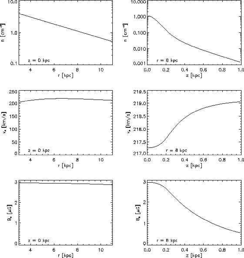
Figure 1.— Density, circular velocity and magnetic field in the initialization. Left panels show midplane quantities versus radius. Right curves show vertical distributions at $r=8\mbox{~{}kpc}$. The gas is initially in hydrostatic equilibrium, with the midplane density decaying radially with a scale length of $4\mbox{~{}kpc}$. The velocity curve is basically flat, increasing only marginally with $z$ to accommodate the radial magnetic tension. The magnetic field is fully azimuthal only in the initialization.

This initialization yields the distribution presented in Figure 1. With slightly different parameters ($p_{M}=1.75\times 10^{-12}$ and $T=5700~{}\mbox{K}$), the vertical density at the solar circle would closely resemble the one described in Boulares & Cox (1990). We chose to use a lower magnetic pressure because we expected that the accumulation of the gas in the spiral arms would increase the magnetic field to values closer to those observed. Also, we expected that the gas dynamics could possibly generate a random component of the field; this did not occur. There are several possible reasons: low spatial resolution, numerical diffusivity, a low effective Reynolds number, a near laminar flow, or a combination of all. We chose to use a higher temperature to help offset the smaller magnetic pressure (this was necessary because, without the extra pressure, the density drops very fast with $z$, generating numerical problems). It should be noted that our relatively high “thermal” pressure is a rough approximation to the pressures provided in fact by the random field, cosmic rays, subgrid turbulence, and the comparatively weak true thermal pressure. Since this pseudo-thermal component is isothermal (except at high density, see discussion below), it did not add the stiffness to the medium that the random field or other components would have. As a result, we likely under-represent the jump-like character of the flow and the associated vertical and turbulent motions.

The rotation curve versus $r$ is nearly flat, increasing only slightly with $z$. From Equation 1, the Alfvén velocity increases with distance from the midplane, to an asymptotic value of about $30\mbox{~{}km s}^{-1}$.

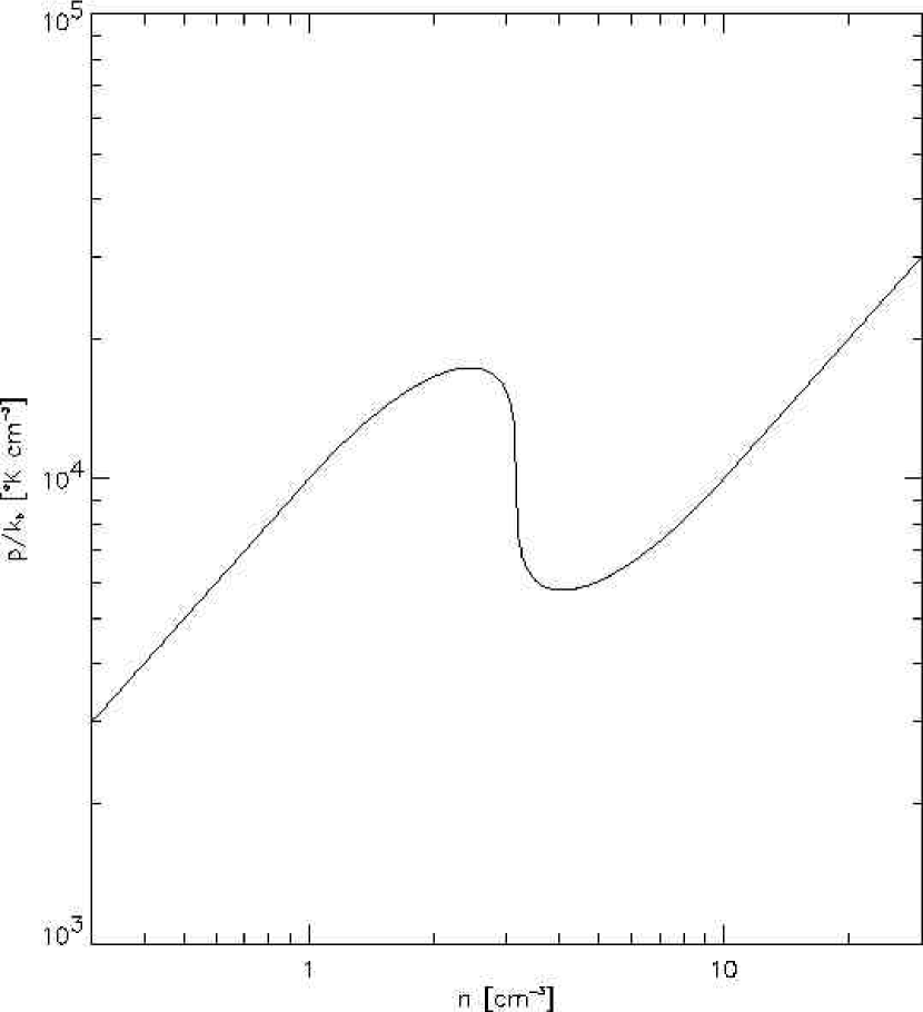
Figure 2.— Equation of state used after the simulation started. Below $n=1\mbox{~{}cm}^{-3}$ and above $n=10\mbox{~{}cm}^{-3}$, the gas is isothermal with $T=10^{4}~{}\mbox{K}$ and $T=10^{3}~{}\mbox{K}$, respectively. In the middle, the temperature falls, mimicking abrupt cooling, and generating a thermally unstable regime.

After the simulation started, we changed the equation of state in order to facilitate the condensation of the gas into the spiral arms. Gas with $n<1\mbox{~{}cm}^{-3}$ behaves isothermally with $T=10^{4}~{}\mbox{K}$; at higher densities, the temperature of the gas is forced down, generating a thermally unstable regime, up to a density of $10\mbox{~{}cm}^{-3}$, above which the gas behaves isothermally again, with $T=10^{3}~{}\mbox{K}$, effectively forming a two-phase medium (Figure 2). This change will have the biggest effect near the midplane, where thermal pressure dominates the magnetic pressure. The choice of $10^{3}~{}\mbox{K}$, rather than $\sim 10^{2}~{}\mbox{K}$ that one might expect from the heating-cooling balance, was made because this pseudo-thermal pressure represents other components that cannot be radiated away, and because of our coarse resolution. It is a modest attempt to sample the effects of condensation, either due to reduced thermal pressure or self-gravity.

In contrast to Paper I, the calculation is performed in the reference frame of the spiral perturbation, which moves with an angular velocity of $12\mbox{~{}km s}^{-1}\mbox{~{}kpc}^{-1}$. The perturbation locus is a logarithmic spiral with a pitch angle of $15^{\mbox{\small o}}$. In radius, the potential perturbation varies in such a way that the implied density perturbation decays exponentially with a scale length of $8\mbox{~{}kpc}$. In azimuth, the perturbation is sinusoidal, with a peak-to-valley amplitude corresponding to an arm/interarm mass ratio of 3.16 at $r=8\mbox{~{}kpc}$. In the midplane, the perturbation force is a relatively constant fraction, $\sim 7\%$, of the average radial force. Details of the radial and vertical shape of the perturbation are presented in Cox & Gómez (2002).

The perturbation is turned on linearly during the first $50\mbox{~{}Myr}$ of the simulation. Also, to avoid splashing against the inner radial boundary, the perturbation forces are not applied in the $3\mbox{~{}kpc}<r<4\mbox{~{}kpc}$, and smoothly increase to full strength in the next kpc. Therefore, the actual useful grid extends from 5 to 11 kpc.

In summary, the differences between the models presented here and those of Paper I are: the new equation of state, a higher magnetic pressure in the initialization, and the shift of the calculation to the pattern reference frame. Also, in order to avoid some of the numerical problems described in Paper I, we set a density floor of $n=4.75\times 10^{-9}\mbox{~{}cm}^{-3}$, equal to the minimum density in the initialization. We were consequently able to run the simulation to much greater ages.

The setup described should be susceptible to the Parker instability (Parker, 1966). Nevertheless, we do not expect to see the interchange mode of the instability due to our low resolution, while the undular mode is expected to be quenched by both our lack of resolution and the flow we are modeling. In order to test this expectation, we restricted the computational domain to a two-dimensional grid along the solar circle, and set up an atmosphere like the one described above. When we turned the arm perturbation off, we observed the growth of the undular mode of the Parker instability. But, when the perturbation was added, the magnetic field lines bent due to the vertical motion of the gas generated by the hydraulic jump, and not so much by the weight of the gas. So, any vertical perturbation in the magnetic field will be carried along with the orbiting gas, and will be damped out when it encounters the hydraulic jump. Therefore, as long as the arm-encounter time is shorter than the instability growth time scale, the undular mode of the instability should not be present.

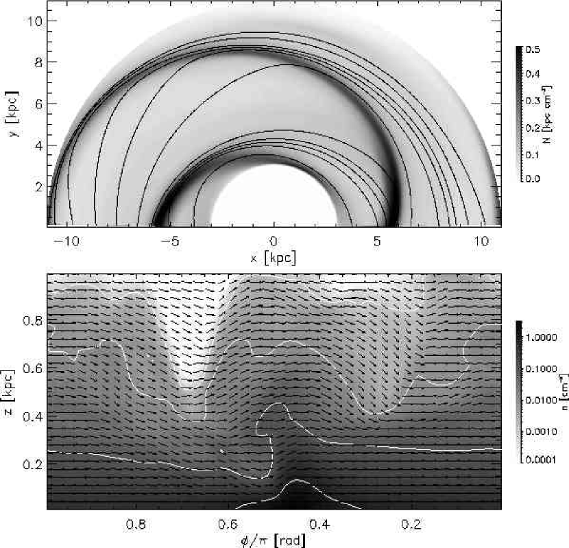
Figure 3.— Structure of our two-arm case after $800\mbox{~{}Myr}$. In the upper panel, the grayscale shows the half-disk column density, and the lines show the integrated pattern frame velocity field in the midplane. In the lower panel, the grayscale show a density cut along a cylindrical surface at $r=8\mbox{~{}kpc}$ with contours at each decade, down from $n=1\mbox{~{}cm}^{-3}$. The arrows show the velocity field component parallel to that surface, in the pattern reference frame. Since ours is a trailing spiral, the gas flows clockwise in the upper panel, and from left to right in the lower one. In the bottom panel, the gravitational perturbation potential minimum occur at $\phi/\pi=0.5$.

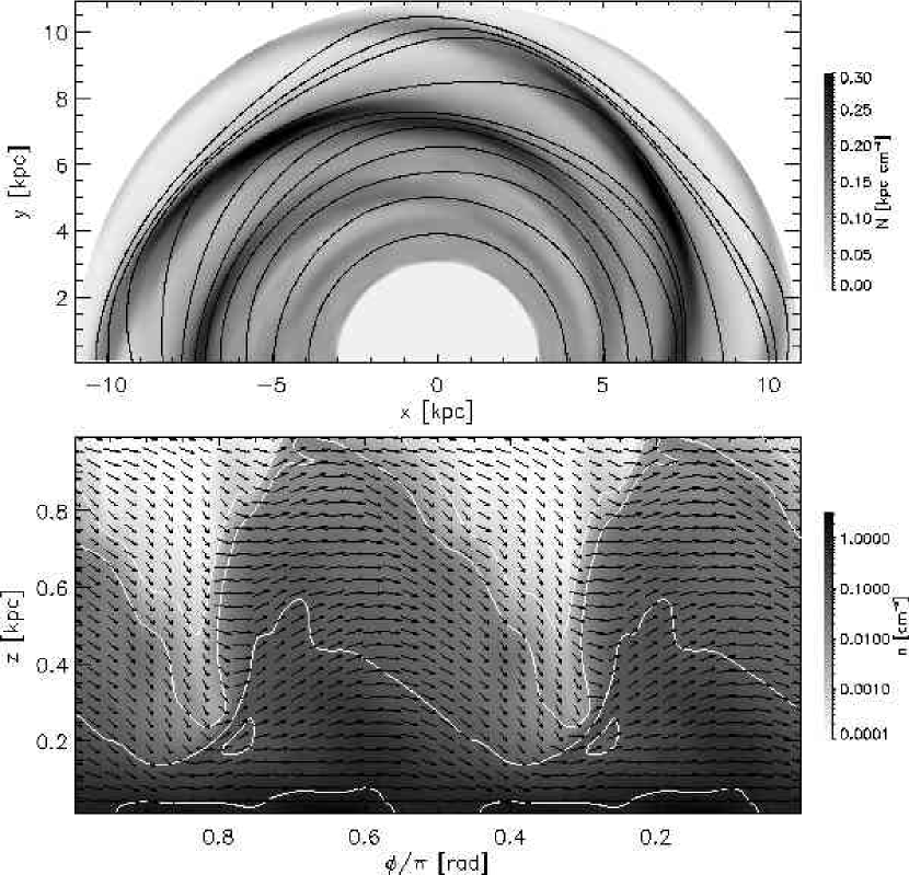
Figure 4.— Same as Figure 3, for our four-arm model. In the bottom panel, the gravitational perturbation potential minima occur at $\phi/\pi=0.35$ and $0.85$.

2.1. General behavior of the simulations.

Figures 3 and 4 show the structures of our two standard models (two and four arms) after 800 Myr. (Unless otherwise noted, we report the state of the simulations at this time.) In both Figures, the grayscale in the upper panel shows half-disk column density; the solid lines show the integrated pattern frame velocity field in the midplane. The grayscale in the lower panels shows a density cut at a cylindrical surface with $r=8\mbox{~{}kpc}$. The arrows represent the velocity field in the pattern reference frame. The length of the arrows is proportional to the total velocity in the $r=8\mbox{~{}kpc}$ surface; but, since the vertical axis is greatly stretched (in reality, the aspect ratio of the grid is $r\Delta\phi:\Delta z\approx 24:1$) the individual components of the velocity are also stretched so that the arrows point in the corresponding direction with respect to the density structures. As these are models of trailing spirals, the gas rotates clockwise in the upper panels, and from left to right in the lower ones.

In Paper I, we showed that, as the gas enters the arm, a combination of a shock and a hydraulic jump is formed. The extra stiffness the magnetic field adds to the ISM makes the gas jump over the obstacle the gaseous spiral arm represents. The gas shoots up before the arm, forming an forward leaning shock, and falls back down after the arm, generating a secondary shock. In isothermal cases with no magnetic field (Paper I), there is much less vertical motion, the forward shock is nearly vertical, and there is no secondary shock.

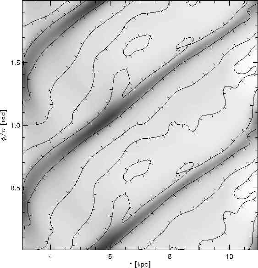
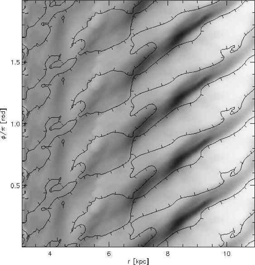
Figure 5.— Integrated vertical mass flux for the two-arm case (left panel) and the four-arm case (right panel). In both panels, the grayscale shows the column density of the simulation. The contour shows the zero-level of the vertical flux, with the dashes pointing in the downflow direction. The gas flows up at the arms and down in the interarms. The two-arm case has a second up-down structure in the interarm region. In both cases, there is a tendency for frequency doubling around $r=7\mbox{~{}kpc}$. Gas flows down from the top.

2.1.1 Two arm model.

In the two-arm case, when the gas falls behind the arm, it bounces back up generating a high $z$ interarm structure that mimics another arm. The high $z$ material then falls again before reaching the next arm. This structure does not show up in the column density, but it is clear in both velocity and density in the lower panel of Figure 3. It is explored in the left panel of Figure 5, where the contours show the zero-level of the integrated vertical mass flux ($\int\rho v_{z}~{}dz$), with the dashes pointing in the downflow direction. The column density is shown in grayscale. The downflow region is broader and happens at lower densities than the upflow. Also, there is a second upflow region downstream of the arm, that mimics the flow structure around the arm. A powerful bounce therefore appears to be a mechanism that might double the number of gaseous arms relative to the stellar arms, as is apparently observed in some galaxies.

Generally speaking, in contrast with the model of Roberts (1969), the gaseous arms sit downstream from the perturbation minimum, but follow a tighter spiral (with a pitch angle of about $13^{\mbox{\small o}}$). We have not yet discovered the reasons behind either the pitch angle difference (which appears in both 2D and 3D models) or the phase difference relative to Roberts (1969) result.

2.1.2 Four arm model.

The four-arm case (Figure 4) has a similar structure to the two-arm one, but presents a big difference: when the gas falls behind the arms, it does not have enough space to complete a bounce and fall again before it encounters the next arm. The downflow does lead to vertical compression ahead of the next arm, but not to a doubling of the vertical velocity pattern. The leading shock is also more vertical, especially at higher $z$. The right panel in Figure 5 shows the vertical mass flux for the four-arm case. Here, the upflow region is broader than in the two-arm case and, as noted above, there is no obvious interarm bounce structure. (Both two and four-arm models show higher numbers of features in narrow radial ranges, notably around $r=7\mbox{~{}kpc}$. This may be due to a resonance between vertical oscillations and arm passage time, and is associated with broadening or even doubling of the arm structure.)

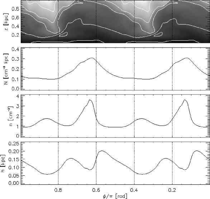
Figure 6.— Comparison of the azimuthal extension of the arms for $r=8\mbox{~{}kpc}$ in the four-arm model. Starting from the top, the first panel shows the density on a surface at constant radius, with contours at every decade, starting at $1\mbox{~{}cm}^{-3}$. The second shows the half-disk column density, the third shows the midplane density, and the last panel shows the disk scale height, defined as the ratio of the column to midplane densities.

It is not clear how to separate the arm and the interarm regions. We illustrate this in Figure 6. As shown in the top panel (a reproduction of the lower panel of Figure 4), the high $z$ structure associated with a spiral arm is very wide, as traced by the density contours. In fact, the region over which the disk thins (the contours reach low $z$) is very narrow. On the other hand, the column density (second panel from the top) also has clearly defined arms, but they cover a smaller region in azimuth than the high $z$ density structure. The arms are even narrower when we look at the midplane density (third panel from the top). Notice that, even if the gas flow does not bounce in the interarm, the downflow compresses the disk and generates an overdensity near the midplane before it encounters the next arm.

A frequently used measure for the thickness of the disk is the ratio of the column density to the midplane density, which is an estimate of the scale height. Examination of the top panel of Figure 6 leads to the idea that the disk swells at the arms. But, since the arm characteristics have different extents along azimuth, the estimated scale height (bottom panel) has a local minimum in the middle of the arm. In the leading and trailing end of the arm, the scale height increases, as expected. This difference in the behavior of the column and midplane densities causes the scale height defined in this way to behave counter-intuitively.

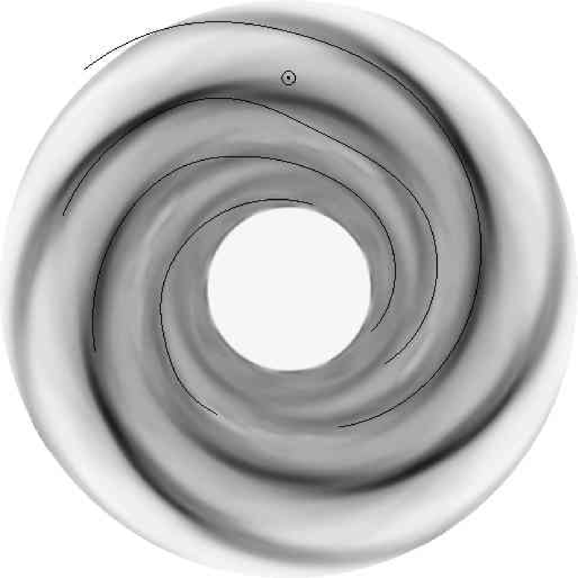
Figure 7.— Column density of our four-arm model, compared with the positions of the Milky Way’s arms, as traced by Taylor & Cordes (1993). The position of the Sun with respect to the modeled arms is marked.

In Figure 4 the arms seem to be discontinuous, with a break at about $r=7.5\mbox{~{}kpc}$. Each of the sections follows an even tighter spiral (with $11^{\mbox{\small o}}$ pitch angle) than the perturbation ($15^{\mbox{\small o}}$) and the overall locus of the arm ($13^{\mbox{\small o}}$). The locus pitch angle has the advantage that the resulting arms are a good approximation to the Milky Way’s spiral arms as traced by Taylor & Cordes (1993). Figure 7 shows the column density of our four-arm model and the locus of the arms in the aforementioned work, scaled so that the distance from the Sun to the Galactic center is $8\mbox{~{}kpc}$. This agreement is extensively used in Gómez & Cox (2004), where we generate synthetic observations using this model, for comparison with real Milky Way data.

3. Magnetic field.

Figures 3 and 4 show that, as material in the midlpane approaches the arms, it moves radially outward, then shocks and follows a path nearly parallel to but soon outside of the arm, moving radially inward in the process. As we discuss below, the post shock inward flow at the midplane is smaller than the outward preshock excursion, and there is a slight migration outward balanced by inflow at higher $z$.

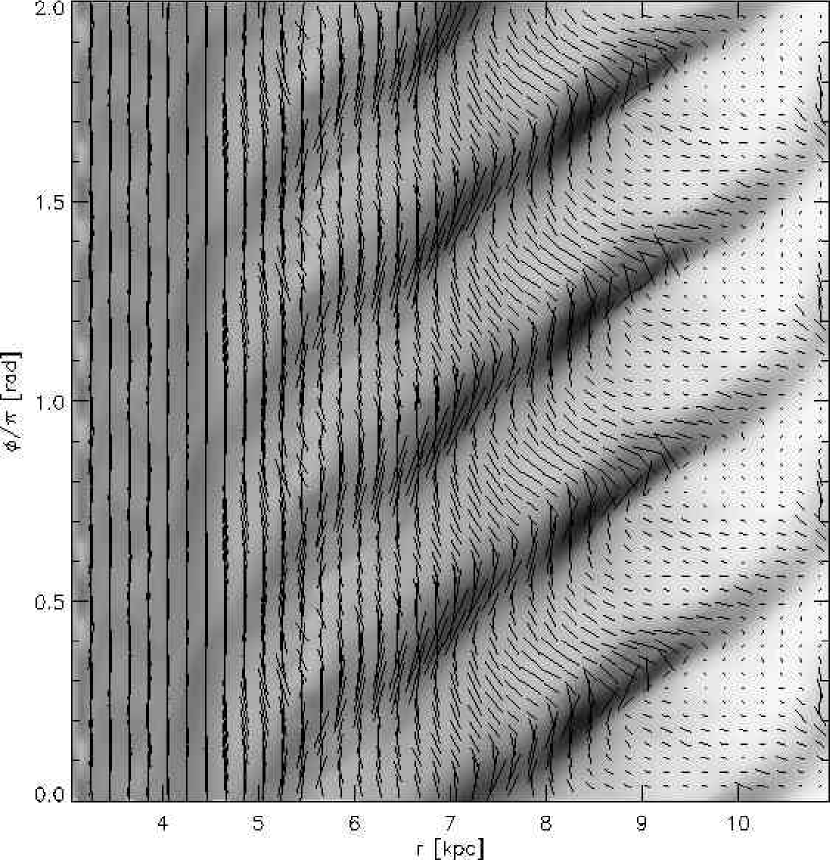
Figure 8.— Pitch angle of the magnetic field in the midplane for the four-arm case and its relation with column density. The grayscale shows the column density of the gas, while the lines show the direction of the magnetic field, with length proportional to the intensity in that plane. As with Figure 5, the gas flows down from the top.

Figure 9.— Same as Figure 8, for $z=0.5\mbox{~{}kpc}$. The length of the lines (proportional to the field strength) have the same normalization as in Figure 8. Patches where the field strength is very small must lie in regions where the higher $z$-lower field material has moved downward to this level. Conversely, strong fields are present where the stronger field from below has been advected upward. A sudden jump from one to the other occurs on the leading edges of the arms for $r>7\mbox{~{}kpc}$.

The magnetic field is carried along with this flow, and therefore has a radially outward component ahead of the arms and a radially inward component just outside of them. On Figure 8, these radial excursions of the field lines are plainly seen. At the locations of the arms, the field is roughly parallel to the arm locus. Between the arms, the field pitch changes from somewhat less positive than the arm pitch, to circular, to negative pitch as it approaches the next arm.

At higher $z$ (Figure 9), both the velocity pattern and field structure are somewhat less regular. As expected from the gas flow, the largest vertical component of the magnetic field is found just before and after the arms. The vertical field can be as large as $0.4\mu\mbox{G}$, but $0.2\mu\mbox{G}$ is a more typical value.

The two-arm case (not shown) has a much smoother magnetic field. It can also show negative pitch in the interarm region, but it does not change as abruptly as in the four-arm case. Also, the vertical field is weaker, being prominent only on the leading edge of the gaseous arms.

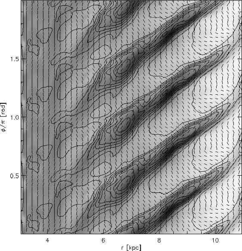
Figure 10.— Synchrotron emission of the four-arm model. Grayscale shows the gas column density, while the contours show the intensity of the emission. Dashes show the direction of the magnetic field as inferred from the polarization.

3.1. Synchrotron emission.

Owing to our missing the random field component, a synthetic synchrotron map cannot represent the emission actually expected from a galaxy, but it could provide a reasonable view of the polarized fraction. Figure 10 shows our calculated total emission, for our four-arm case, as viewed from outside the galaxy, with lines showing the directions of the apparent field (perpendicular to the $E$ field polarization of the integrated emission), assuming no Faraday rotation.

At any given distance above the plane, the emissivity is given by:

$$\varepsilon_{tot}(r,\phi)\propto n_{e}(r,z)B_{\perp}^{(p+1)/2},$$ (2)

where $B_{\perp}$ is the component of the field parallel to the plane of the galaxy, $p=2.5$ is the spectral index of the electron cosmic ray distribution, $n_{e}(r,z)=\exp(-r/r_{cr}-z/z_{cr})$ is the spatial distribution of the electron cosmic rays, $r_{cr}=13\mbox{~{}kpc}$, and $z_{cr}=2.5\mbox{~{}kpc}$ (Ferrière, 1998). This emissivity is integrated along a line of sight perpendicular to the galactic plane. The polarization is calculated by estimating the polarized emission parallel and perpendicular to $B_{\perp}$,

$$\varepsilon_{\parallel} = \frac{1+\Pi}{2}\varepsilon_{tot}$$ (3)

$$\varepsilon_{\perp} = \frac{1-\Pi}{2}\varepsilon_{tot},$$ (4)

where $\Pi=(p+1)/(p+7/3)$ is the degree of polarization of the emissivity. Given the angle $\alpha$ and the intensities $I_{tot}$, $I_{\parallel}$ and $I_{\perp}$ at a certain $z$, the intensities and parallel direction at $z+dz$ are given by:

$$\alpha^{\prime} = \alpha$$

$$+\frac{1}{2}\mbox{arctan}\left[\frac{(\varepsilon_{\perp}-\varepsilon_{\parallel})dz\sin[2(\beta-\alpha)]}{(I_{\perp}-I_{\parallel})+(\varepsilon_{\perp}-\varepsilon_{\parallel})dz\cos[2(\beta-\alpha)]}\right]$$

$$I^{\prime}_{tot} = I_{tot}+\varepsilon_{tot}dz$$ (6)

$$I^{\prime}_{\parallel} = I_{\perp}+\varepsilon_{\perp}dz-(I_{\perp}-I_{\parallel})\cos^{2}(\alpha^{\prime}-\alpha)$$ (7)

$$-(\varepsilon_{\perp}-\varepsilon_{\parallel})dz\cos^{2}(\alpha^{\prime}-\beta)$$

$$I^{\prime}_{\perp} = I^{\prime}_{tot}-I^{\prime}_{\parallel},$$ (8)

where $\beta$ is the direction parallel to the magnetic field at $z+dz$. Notice that $\alpha^{\prime}$ is not the direction of polarization nor the direction of the magnetic field, but the direction of the inferred B-field, as traced by the synchrotron emission.

In Figure 10 we can see that the interarm turning of the B-field happens around the area of minimum emission, which is consistent with the picture of being a consequence of stretching the field. The higher intensity regions tend to be slightly upstream from the arm. The degree of polarization is quite large (about 70%). This is expected, since our resolution does not allow us to model the random component of the field, that might depolarize the emission. Only a shift in the direction of the B-field with $z$ reduces the polarization from the $72.4\%$ of the intrinsic emissivity.

For our two-arm case (not shown), the polarization changes are not as abrupt, the arms are more continuous (no blobs with associated peaks of synchrotron emission), and the difference in the positions of the peaking of emission and column density is smaller.

Figure 10 is to be compared with the maps from Beck et al. (2002). In that work, an atlas of synchrotron emission in external galaxies is presented. They compared the polarized and total emissions, as a way of comparing the total (random + regular) and regular B-fields (again, we do not have enough resolution to say much about the random field). They consistently found islands of synchrotron emission and displacements between the synchrotron and gaseous arms not so different from the ones found here. We did not find magnetic arms without a density counterpart, which have been occasionally found in polarized emission observations and some simulations (Elstner et al., 2000, for example).

Galaxies should have a lot of random field in the spiral arms, generated by both the turbulence of the jump and stellar feedback, but the post arm flow should stretch the field to greater regularity in the interarm region. To the extent that this is true, we would expect the mean convected field to follow the pattern just described. Some observations (Han et al., 1999) suggest that in some galaxies there are magnetic arms, regions of enhanced polarized synchrotron emission not associated with the gaseous arms. Our finding that in two-arm spirals, with their longer interarm transit, the flow tends to bounce and generate an arm-like structure in the interarm region could also be related to this phenomenon. A detailed exploration of these points is outside the scope of the present work.

3.2. Magnetic field-density relation.

The relationship between magnetic field strength and density in the interstellar medium is an interesting diagnostic of the behavior of the flow. To the extent that the various components of the ISM are all just the current states of material that samples all states, so that there is no intrinsic relationship between density and flux, the relationship should distinguish the various dynamical possibilities. If the field were small enough to be dynamically insignificant, compressions on average should be three dimensional, which with flux freezing would yield $B\propto n^{2/3}$. If the field were so strong that it dominates the pressure, compressions would be possible only along the field, and there would be no dependence of field strength on density, except in dynamically active environments. Measurements of the field strength in the midplane, at average and lower densities seem to find no dependence of $B$ with $n$ (Heiles, 2001). At densities high enough that local dynamics or self gravity is important, higher field strengths (and higher total pressures) are found (Crutcher, 1999). At the lower densities, some measurements provide only upper limits to local region fields, but the strong fluctuations in pulsar dispersion measures and the overall synchrotron emissivity seem to imply that the rms field is several microgauss. It would appear that most of the volume, even at low density, must have fields of this order (see discussion in Vallée, 1997).

Our simulation can be explored for its $B(n)$ relationship, though some care is required in interpretation. Two factors must be kept in mind. First, we initialize our run with a very strong dependence of $B$ on $n$, as given by Equation 1. It is almost certain that far from the plane of the Galaxy, not only is the density low, but so is the magnetic field. Our initialization is a specific rule for this relationship, and determines the static vertical structure. We observe, however, that even in our relatively laminar flow, material makes large vertical excursions in its response to the arm disturbance (see Section 6). Thus, the material found at any given height will have a wide spread in initial heights, and therefore, a wide spread in initial $B(n)$. This is more true further from the plane, but should not be discounted close to the plane as well.

The second point is that because we do not have a significant random field, it may be easier for material to move along the field than in the actual Galaxy. This is not necessarily true if, for example, most of that motion occurs in interarm regions where the field is less random (as discussed above). It is also possible that in the actual Galaxy, a considerable amount of motion along fields is driven at small scales and high densities by stellar feedback in the arms, and then frozen in as the material and field are stretched out between the arms, the field returning to its pressure defined equilibrium, with whatever distribution of density is left from the small scale dynamics.

In short, the results we are about to present are suggestive, but cannot be assumed to represent reality very precisely.

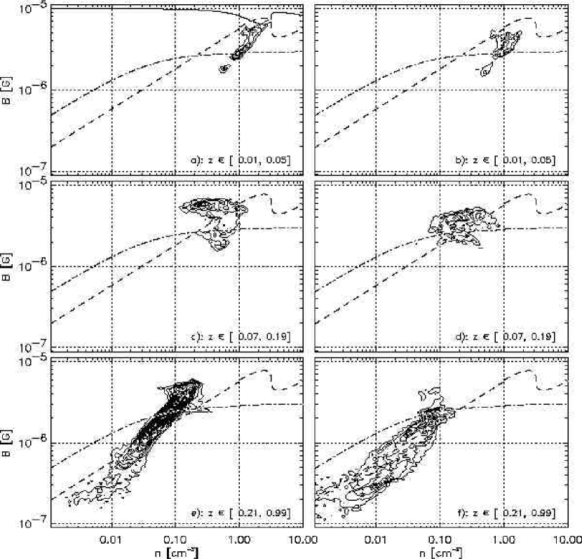
Figure 11.— Distribution of density and magnetic field strength between $r=7$ and $9\mbox{~{}kpc}$ for the four-arm model. The left column corresponds to gas in and near the spiral arms, while the right column corresponds to interarm gas. The solid line in panel $a$ traces the amount of magnetic field needed for a total pressure of $4\times 10^{-12}\mbox{~{}dyn}\mbox{~{}cm}^{-2}$. The dashed line in all panels shows the locus of equal magnetic and thermal pressures. The dot-dash line follows the magnetic pressure-density relation used in the initialization.

Owing to our strong $B(n)$ in the initialization, we restrict our presentation to material found between 7 and $9\mbox{~{}kpc}$, and present three ranges in $z$, close to the plane, intermediate, and high, the boundaries between them being at 50 and $200\mbox{~{}pc}$. We also separate the material into two equal halves (in space), one containing the arms, the other not. The results are shown in the six panels of Figure 11. The contours are of volume containing $B(n)$.

There are also several lines on these diagrams, one showing the $B(n)$ of the initialization, one showing the locus of equal magnetic and thermal pressures, and one (shown only on the midplane arm plot) showing a line of constant total pressure of $4\times 10^{-12}\mbox{~{}dyn}\mbox{~{}cm}^{-2}$.

There are several things to notice. First, at no height does the initial trend of $B(n)$ represent the trend of the data, though in every diagram, significant amounts of material are found along parts of the initialization. Next, there are three characteristic features found in the plots, sections where the distribution has a major horizontal feature, sections where there is a major feature or slope somewhat steeper than the initialization, but lower than the slope (one) expected from purely transverse compression, and in the midplane, a feature at the highest densities which has a concave upward boundary.

The horizontal segments, most noticeable at the intermediate heights, are exclusively found in regions in which the magnetic pressure is higher to significantly higher than the thermal pressure. Our flow thus seems to reproduce the expectation that in such regions the dominance of magnetic pressure is accompanied by flows parallel to it. The vertical width of the horizontal segment should then be associated with the spread in pressures found between 50 and $200\mbox{~{}pc}$ in the central pair of panels. The width is roughly a factor of 1.4 in $B$ and therefore 2 in pressure, more or less consistent with the pressure variation with height presented in Section 4. The fact that this behavior is not well represented in the midplane is likely due to our initialization with dominant thermal pressure at the midplane densities. Notice that in our simulation, the densities within $50\mbox{~{}pc}$ of the midplane are never as low as those expected for intercloud regions in the Milky Way.

The inclined segments have $B\propto n^{0.7}$ or so, roughly as expected from isotropic compression, a little steeper than the initialized relationship. Instead of showing isotropic compression, it could be a mixture of the initialization and the $B\propto n$ expected from purely transverse compression. We do not therefore give definitive reasons for this behavior, but note that it is always found in material whose magnetic pressure is less than or comparable to its thermal pressure. It is in the regime for which isotropic compression is plausible.

The third feature, the concave upward behavior at the highest densities close to the plane, appears to be a consequence of our thermal equation of state. This behavior occurs at those densities for which the temperature is rapidly decreasing with increasing $n$, requiring a higher value of $B$ to have the same total pressure. Notice the similarity of the locus to the constant pressure line superimposed.

4. Vertical hydrostatics.

Various authors (Boulares & Cox, 1990, and references therein) have attempted to reconcile the apparent midplane pressure of the Galaxy with the weight of the material above it. In this section, we test two aspects of this procedure, whether such equality is expected locally (for example, in the immediate neighborhood of the Sun, there appears to be a scarcity of material relative to the average and one might wonder whether this should be reflected in a lower than average midplane pressure), and the degree to which dynamics contributes to the overall balance.

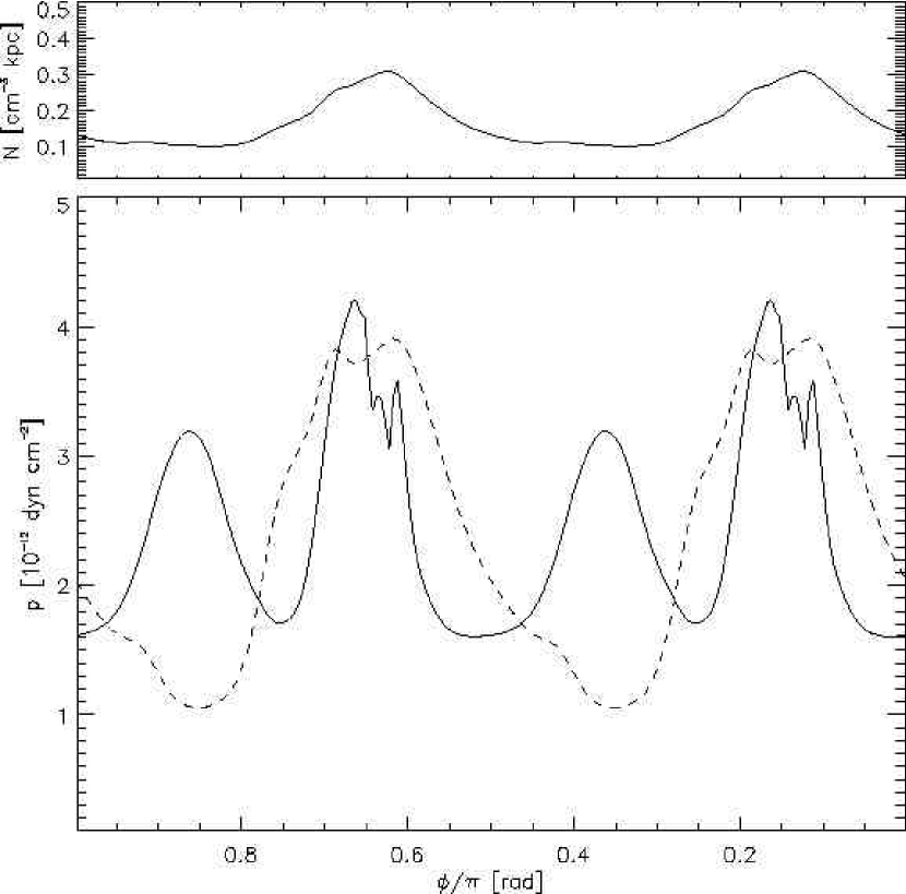
Figure 12.— Comparison of the midplane pressure and gas weight for $r=8\mbox{~{}kpc}$ for the four-arm model. In the lower panel, the solid line shows the midplane pressure, while the dashed line shows the integrated weight. In the places where the weight is higher than the pressure, the downward force is decelerating the upflow (before the arm) or generating the downflow (after the arm). The pressure is higher in the interarm because of the kinematic pressure due to the downflow behind the arm and the subsequent bounce. The half-disk column density is provided in the upper panel for reference.

In Figure 12 we compare the midplane thermal plus magnetic pressure with the integral of the overlying weight per unit area versus phase along a line of constant galactocentric radius of 8 kpc. The half-disk column density is also provided for comparison. The mean value of the midplane pressure ($2.45\times 10^{-12}\mbox{~{}dyn}\mbox{~{}cm}^{-2}$) is in good agreement with the mean weight ($2.41\times 10^{-12}\mbox{~{}dyn}\mbox{~{}cm}^{-2}$). But the behavior with phase shows much more interesting structure. The midplane pressure does have significant variations, as does the weight, and they are correlated to some degree. A perfect match is not expected because material does not evolve on constant radius, because these results are for one specific time, during which things might be slightly out of equilibrium, and because the pressure calculated does not include dynamical contributions. Still, it is possible to get a sense of the dynamical behavior from this plot. For $\phi/\pi=0.8$ to 1, the column density is nearly constant, so the weight is a measure of the vertical extent. From left to right, the weight falls, as does the material, raising the midplane density and pressure. The trend reverses about $\phi/\pi=0.85$ to upflow, increasing weight and decreasing pressure. This is a bounce. Then, there is a sudden increase in pressure and weight, a shock, that raises the pressure above the weight, though only slightly. This is the hydraulic jump. It sustains the upflow, roughly stabilizing the increased height. Thereafter, the flow accelerates parallel to the plane, decreasing the pressure, weight, and column density. Because the effective $\gamma$ is grater than 1, the pressure drops faster than the weight, leading to downflow, a downstream pressure increase and weight minimum, ready to bounce again.

We have explored the vertical hydrostatics more precisely, averaging over phase to see how the contributions to pressure versus height are arranged. We cannot explore the importance of magnetic tension as Boulares & Cox (1990) did, since our model has restrictions that limit the development of vertical magnetic field, namely, lack of spatial resolution, no cosmic rays pushing the magnetic lines, nor an effective dynamo. Nevertheless, we found that the large scale motions of the gas provide a significant fraction of the support.

Consider the vertical component of the momentum conservation equation:

$$\rho\left[\frac{\partial v_{z}}{\partial t}+(\mbox{\boldmath$v\cdot\nabla$})v_{z}\right]=-\rho g_{z}-\frac{\partial}{\partial z}\left(p_{th}+p_{m}\right),$$ (9)

where $v_{z}$ is the component of the velocity in the vertical direction, $g_{z}$ is the vertical gravitational acceleration, $\rho$ is the gas density, $p_{th}$ is the thermal pressure, and $p_{m}$ is the magnetic pressure. Here, we used the approximation proposed in Boulares & Cox (1990), in which the magnetic pressure is diminished by the magnetic tension: $p_{m}=(B^{2}-2B_{z}^{2})/8\pi=(B_{r}^{2}+B_{\phi}^{2}-B_{z}^{2})/8\pi$. In our model, the vertical field is not very large, and the magnetic tension is only a small fraction of the vertical support. In the case of $\partial/\partial t=0$,

$$p(z)=p(z_{0})+\int^{z_{0}}_{z}\rho\left(g_{z}+\frac{v_{\phi}}{r}\frac{\partial v_{z}}{\partial\phi}+v_{r}\frac{\partial v_{z}}{\partial r}+v_{z}\frac{\partial v_{z}}{\partial z}\right)dz.$$ (10)

In Figure 13, the left panel shows the four different integrated terms in the right side of Equation 10, and the right panel compares the left and right hand sides of the equation. In that Figure, $p(z_{0})$ is the value of the thermal plus effective magnetic pressure at the upper boundary at $z_{0}=1\mbox{~{}kpc}$. All the plotted quantities are actually the mean values along the solar circle, so that the effect of the spiral arms is averaged out to give a global picture. In order to calculate the weight of the gas, the total gravitational potential (background + perturbation) was used, but it makes little difference, since the actual value of the perturbation is small compared with the background potential.

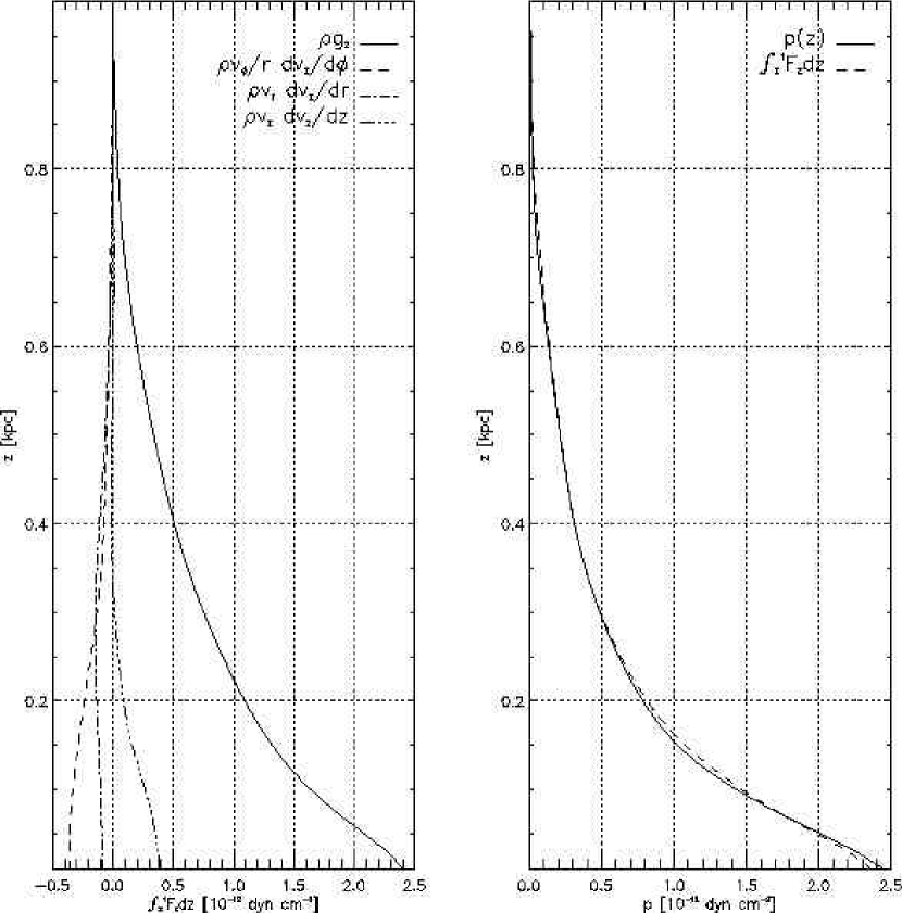
Figure 13.— The left panel shows the contributions of the different force terms to the vertical support of the disk. Notice that the vertical kinematic pressure works in the same direction as the gas weight. The right panel compares the pressure [thermal + magnetic, in the Boulares & Cox (1990) tension approximation] and the vertical forces. When the convective terms are considered, the disk is very close to vertical equilibrium at this epoch.

Figure 13 shows that the spatially averaged disk atmosphere is actually very close to hydrostatic at the $t=800\mbox{~{}Myr}$ time shown. Although most of the pressure is balanced by the weight of the gas, the convective terms have a significant influence, specially at intermediate $z$. As expected, the first two convective terms work into supporting the weight of the gas, generating kinematic pressure. But the fourth term, the vertical kinematic pressure $\int\rho v_{z}(\partial v_{z}/\partial z)dz$, has the same sign as the gas weight. This is because its average is biased toward the highest vertical velocity regions. Such regions are the downflow behind the arms, where $v_{z}$ is negative and becoming more negative with increasing $z$. As hinted by Figure 12, the midplane disk pressure has to decelerate the downflow in addition to supporting the weight of the gas.

At different times, the lines showing the weight of the gas (dashed line in the right panel of Figure 13) and pressure (solid line) oscillate only slightly around each other, suggesting that the vertical hydrostatics described above is not atypical.

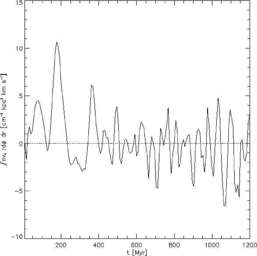
Figure 14.— Vertical mass flux integrated over the plane, at $z=210\mbox{~{}pc}$, as a function of time.

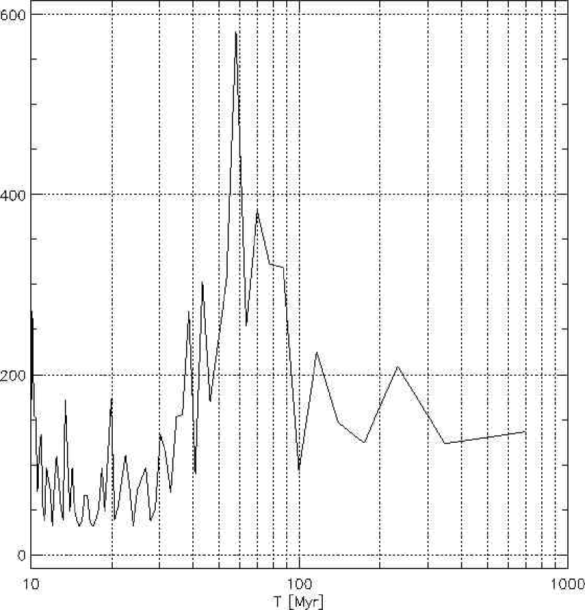
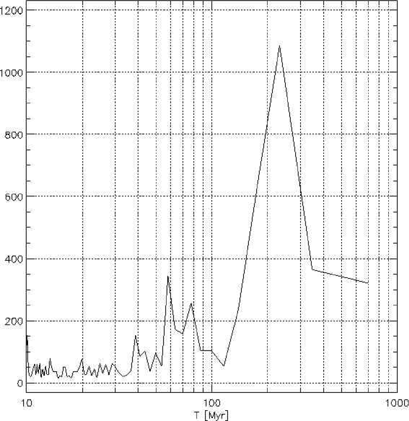
Figure 15.— Fourier analysis for the vertical mass flux at $z=210\mbox{~{}pc}$ for the four-arm case. When we integrate over the plane, a strong peak at $T\sim 60\mbox{~{}Myr}$ appears (left panel). When we restrict the integration to $1\mbox{~{}kpc}$ around $r=8\mbox{~{}kpc}$, that peak diminishes, and another one at $T\sim 230\mbox{~{}Myr}$ appears (right panel).

5. Periodicity.

The simulations do not seem to be in a steady state, but rather in a steady cyclic behavior, in which the “wave-like” structure that is formed above the gaseous arms breaks, only to be regenerated at the back of the arm and rise again. The periodicity of the simulation can be assessed by plotting the vertical mass flow, at a given height, integrated over the $r-\phi$ plane, as a function of time. Such a plot for the four-arm case is presented in Figure 14. The chosen height is $z=210\mbox{~{}pc}$, which is right across the “breaking wave” structure (see Figure 4). The left panel of Figure 15 shows the Fourier transform of this vertical flux for $t>500\mbox{~{}Myr}$. It shows a strong peak at about $T\sim 58\mbox{~{}Myr}$. That peak grows smaller if we restrict the integration to only a range of $1\mbox{~{}kpc}$ around $r=8\mbox{~{}kpc}$ ($1\mbox{~{}kpc}$ is the typical width of the gas’ radial motions, see Section 6). The right panel of Figure 15 shows that case. Notice that a second strong peak at $T\sim 230\mbox{~{}Myr}$ appears. Both peaks are present when we move the integration range to $r=6\mbox{~{}kpc}$ and $10\mbox{~{}kpc}$, although they both move to slightly smaller periods and the large period peak becomes weaker than the short period one as we go to smaller radii.

We performed a linear perturbation analysis of the vertical motions of the disk in order to understand the origin of these periods. The procedure is very similar to the one followed in the appendix of Walters & Cox (2001). Consider the equation of motion in the vertical direction for an plane-parallel isothermal atmosphere:

$$\frac{\partial v}{\partial t}=-\frac{1}{\rho}\frac{\partial p}{\partial z}-g,$$ (11)

where $v$ is the velocity, $\rho$ is the mass density, $p$ is the total pressure (thermal plus magnetic), and $g=\partial\Phi/\partial z$ is the gravitational acceleration. Consider perturbations to the (hydrostatic) equilibrium distribution,

$$\rho\longrightarrow \rho_{0}+\delta(z)$$ (12)

$$p\longrightarrow p_{0}+\epsilon(z)$$ (13)

$$v\longrightarrow v(z).$$ (14)

Substituting these into equation 11, and eliminating the hydrostatic equilibrium condition, we get:

$$\frac{\partial v}{\partial t}=-\frac{1}{\rho_{0}}\left(\delta g+c^{2}\frac{\partial\delta}{\partial z}+\delta\frac{\partial c^{2}}{\partial z}\right),$$ (15)

where $c^{2}=\partial p/\partial\rho$. Using mass conservation,

$$\frac{\partial\delta}{\partial t}=-v\frac{\partial\rho_{0}}{\partial z}-\rho_{0}\frac{\partial v}{\partial z},$$ (16)

and assuming that $\delta,v\sim\exp(i\omega t)$, we can eliminate $\delta$ to get,

$$v^{\prime\prime}-v^{\prime}\left[\frac{g+(c^{2})^{\prime}}{c^{2}}\right]+v\left[\frac{\rho_{0}^{\prime\prime}}{\rho_{0}}-\left(\frac{g+(c^{2})^{\prime}}{c^{2}}\right)^{2}+\frac{\omega^{2}}{c^{2}}\right]=0,$$ (17)

where $f^{\prime}=df/dz$. (Notice that this equation reduces to a sound equation for very large frequencies.) Equation 17 can be solved numerically for the initial density and pressure conditions of the simulation, for a given frequency $\omega$. We explored a range of values for $\omega$ and looked for solutions to equation 17 that are consistent with the zero vertical velocity boundary conditions we imposed in the simulation. The lowest frequency consistent with the boundary conditions corresponds to a period of about $50\mbox{~{}Myr}$ for the vertical gravity and density structure at $r=8\mbox{~{}kpc}$. As with the analysis from Figure 15, that period decreases as we move inward ($45\mbox{~{}Myr}$ at $r=6\mbox{~{}kpc}$), and increases outward ($70\mbox{~{}Myr}$ at $r=10\mbox{~{}kpc}$). We did not find a period corresponding to the other $\sim 230\mbox{~{}Myr}$ peak, which could involve radial motions.

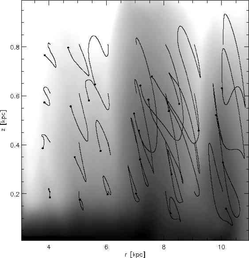
Figure 16.— Paths of gas particles as they move from $\phi=\pi/2$ to $\phi=0$ in the four-arm case, ending at the position with the dot. The grayscale is the logarithm of the density at those angles. The main difference between the looping behavior at low $z$ and the prostate “s” shapes higher up is that, at minimum height, the low $z$ material is moving outward, while the high $z$ material is moving inward. In all cases, the general trend is outward when falling (approaching an arm) and inward when rising (within an arm).

6. Circulation.

In this section, we look for global trends in the gas motions to explore circulation and radial motions of the material. In order to do so, we averaged all the velocities and densities of the simulation for the period of $600-1000\mbox{~{}Myr}$. Then, we integrated the resulting mean velocity field in order to get the trajectory of an imaginary test particle. The result for the four-arm case is presented in Figure 16. In this, the grayscale is the time averaged density at $\phi=0$. The lines show the trajectory in $r$ and $z$ that a test particle follows in the mean velocity field in going from $\phi=0$ to $\pi/2$ (one arm encounter time, which differs with radius), ending at the position with the larger dot.

The first thing to notice in this diagram is that, as the gas goes between arm and interarm regions, it moves a typical distance of about $1\mbox{~{}kpc}$ in $r$, and a varying amount in $z$; sometimes, the vertical displacements can be as large as $0.5\mbox{~{}kpc}$. Also, the trajectories have a slanted appearance. This is consistent with what has been mentioned before: at the spiral shock, the gas shoots up and then moves radially inward along the arm. After leaving the arm, the gas falls down and moves out in radius as it approaches the next arm. The difference between the roughly looping orbits seen at low $z$ and the prostrate “s” shapes at higher $z$ is that material at low $z$ is moving outward at minimum height, whereas at high $z$ it is moving inward. Reference to Figure 4 shows that, at low $z$, minimum height occurs at the interarm bounce, where material is moving outward, while at high $z$, minimum height occurs downstream of the leading edge of the arm, where material has already begun to move in.

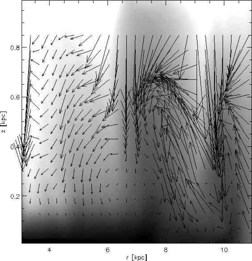
Figure 17.— Same as in Figure 16, but showing the net displacement of the particles for a $\Delta\phi=\pi/2$ fraction of their orbit. The arrows point from to the initial to the final positions. A counterclockwise cycle around the arms can be seen.

In Figure 17, we plotted an arrow from the initial to the final positions of the test particle. The interpretation of this diagram is not straightforward. Each parcel is followed through one fourth of a rotation, relative to the pattern. It typically ends up at both a different $z$ and $r$, and at a different $r$ it is in a different phase with respect to the arm, as evidenced by the shift relative to the density distribution shown. The pattern is also incomplete, in that it shows no obvious source of replenishment for material above $600\mbox{~{}pc}$ outward of $6\mbox{~{}kpc}$. What is clear is that there is a general circulation pattern counterclockwise about each arm structure, in which material above $200\mbox{~{}pc}$ has large radial and vertical net excursions. Higher $z$ material tends to move inward, and lower $z$ outward, though at lower velocity and higher density. In the upper regions of the inner edge of each arm, there is some indication of inward motion that transits from one arm to the next, but we are reluctant to conclude, from modeling by this Eulerian code, that there is thorough mixing of material across the disk.

The fact that the net circulation pattern has several cells, one associated with each arm, shows that it is not a simple consequence of our closed inner and outer boundaries, which might have led to a single cell of circulation.

This Figure is ambiguous about what happens to material very close to the plane, leading us to study the average radial velocity of material as a function of $z$. We calculated the mean radial velocity of the gas at different heights by averaging the radial velocity at a given $z$, weighted by the density at that point:

$$\bar{v}_{r}(z)=\frac{\int\rho v_{r}~{}rd\phi~{}dr}{\int\rho~{}rd\phi~{}dr}.$$ (18)

In Figure 18, we present this mean radial velocity for the time averaged four-arm case. The velocities are inward and significant above $100\mbox{~{}pc}$, reaching $-4\mbox{~{}km s}^{-1}$ at about $400\mbox{~{}pc}$. Near the plane they are outward and low, only about $1\mbox{~{}km s}^{-1}$ is reached. This is consistent with the observational limits (Portinari & Chiosi, 2000, and references therein) and inferences from the previous Figure.

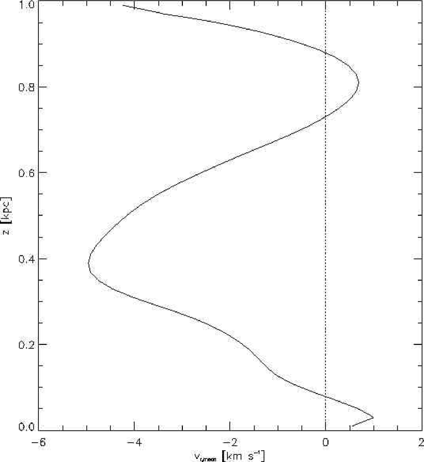
Figure 18.— Mean radial velocity for the time-averaged four-arm case. The gas moves in above and along the arms, and out in the interarm region, closer to the plane similar to the magnetic field pattern in Figure 8. The region of slight positive velocity at $z=0.8\mbox{~{}kpc}$ involves very little material.

From this, we conclude, as anticipated, that there is net outward flow close to the plane to compensate the net inward flow at higher $z$. But we are still uncertain whether this flow occurs in essentially closed cells, separately mixing material within each arm, as suggested by Figure 17 for most of the material, or whether there is sufficient transit between arms for substantial global mixing. Our tentative conclusion is that the velocities shown in Figure 18 are dominated by closed cell circulation, and therefore represent a strong limit on the global mixing rate.

7. Conclusions.

We performed MHD simulations of the gaseous galactic disk having spiral gravitational perturbations with two and four arms. As found in Martos & Cox (1998) and Paper I, the gas motions involve vertical bouncing, plus a combination of a shock and a hydraulic jump at the gaseous arms. The comparative timescales for bouncing and interarm passage, and the realtive phases lead to complications in the details of the arm structure, as predicted by Martos & Cox (1998) and Walters & Cox (2001). This bounce/shock/jump structure leans upstream above the plane, more noticeably in the two-arm case, where the bounce point occurs within the arm at low $z$. In the four-arm case, the low $z$ bounce point occurs at the interarm density peak (at $z=0$) and the upward motion from the bounce leads the shock/jump structure. In both cases, the gas moves up and over the midplane arm, inward in radius. The higher $z$ material then falls down behind the arm, where it is again moving radially outward. In the two-arm case, the gas bounces back up and, at high $z$, generates structures similar to those at the arm, as if the gas were trying to develop a four-arm structure. In the four-arm case, if the Sun’s position is properly chosen, the arms seem to follow the arms traced by Georgelin & Georgelin (1976). In both cases, the gaseous arms follow a spiral tighter than the imposed perturbation.

Since the net radial inflow happens above the arms, and the gas falls in the interarm, when it is moving out before encountering the next arm, the disk averaged radial flow changes sign with height above the disk, from positive near the midplane, to negative higher up. This cycle appears to happen in cells associated with the arms, and might not represent a global mixing phenomenon.

Within the spiral arms, the magnetic field adopts a pitch angle similar to that of the arms, but it develops a negative pitch in the interarms. The vertical magnetic field is only important at the position of the largest vertical flows. Our model does not include cosmic rays, supernovae or other energetic events, and therefore, it does not develop much vertical field, and the total field strength falls faster with $z$ than observations suggest. Those shortcomings, on top of our low resolution, did not allow us to model the random component of the field, which causes us to overestimate the synchrotron polarization fraction.

An examination of the relationship between $B$ and $n$ found that, when the magnetic pressure strongly exceeded the thermal, $B$ was constant, independent of $n$. Conversely, when thermal pressure is significant, $B$ tends to increase with $n$.

The disk atmosphere is close to hydrostatic equilibrium, when the dynamical terms are taken into account. It is noticeable that the downward vertical ram pressure of the gas, when averaged in azimuth, plays an important role in the hydrostatics, incrementing the effective weight of the gas. Magnetic tension plays only a small part in the vertical support, an effect of the model’s weak vertical fields, that may not represent the true situation.

The periodicity of the structures found in this model can be estimated by Fourier analyzing the vertical mass flux. We found two outstanding periods, $T\sim 60$ and $\sim 230\mbox{~{}Myr}$, the smaller of which can be explained in terms of the lowest normal mode of vertical oscillation.

Modelers have the huge advantage of knowing exactly where material being studied is, and its velocity. Observers do not have that luxury. We will make that connection for our model in Gómez & Cox (2004), in which we generate synthetic observations, and then explore them from the advantageous point of knowing the details of the underlying distributions.

References

- Alfaro et al. (2001) Alfaro, E. J., Pérez, E., González Delgado, R. M., Martos, M. A., and Franco, J. 2001, ApJ, 550, 253
- Beck et al. (1996) Beck, R., Brandenburg, A., Moss, D., Shukurov, A., and Sokoloff, D. 1996, ARA&A, 34, 155
- Beck et al. (2002) Beck, R., Shoutenkov, V., Ehle, M., Harnett, J. I., Haynes, R. F., Shukurov, A., Sokoloff, D. D. and Thierbach, M. 2002, A&A, 391, 83
- Block et al. (1994) Block, D. L., Bertin, G., Stockton, A., Grosbøl, P., Moorwood, A. F. M. and Peletier, R. F. 1994, A&A, 288, 365
- Boulares & Cox (1990) Boulares, A., and Cox, D. P. 1990, ApJ, 365, 544
- Cox & Gómez (2002) Cox, D. P. and Gómez, G. C. 2002, ApJS, 142, 261
- Crutcher (1999) Crutcher, R. M. 1999, ApJ, 520, 706
- Dame et al. (1986) Dame, T. M., Elmegreen, B. G., Cohen, R. S., and Thaddeus, P. 1986, ApJ, 305, 892
- Dehnen & Binney (1998) Dehnen, W. and Binney, J. 1998, MNRAS, 294, 429
- Drimmel (2000) Drimmel, R. 2000, A&A, 358, L13
- Edgar & Savage (1989) Edgar, R. J. and Savage, B. D. 1989, ApJ, 340, 762
- Elstner et al. (2000) Elstner, D., Otmianowska-Mazur, K., von Linden, S. and Urbanik, M. 2000, A&A, 357, 129
- Ferrière (1998) Ferrière, K. 1998, ApJ, 497, 759
- Georgelin & Georgelin (1976) Georgelin, Y. M. and Georgelin, Y. P. 1976, A&A, 49, 57
- Gómez & Cox (2002) Gómez, G. C. and Cox, D. P. 2002, ApJ, 580, 235 (Paper I)
- Gómez & Cox (2004) Gómez, G. C. and Cox, D. P. 2004, ApJ, submitted
- Han et al. (1999) Han, J. L., Beck, R., Ehle, M., Haynes, R. F. and Wielebinski, R. 1999, A&A, 348, 405
- Heiles (2001) Heiles, C. 2001 in ASP Conf. Ser. 231, Tetons 4: Galactic Structure, Stars, and the Interstellar Medium, ed. C. E. Woodward, M. D. Bicay, & J. M. Shull (San Francisco: ASP), 294
- Lin & Shu (1964) Lin, C. C. and Shu, F. H. 1964, ApJ, 140, 646
- Lindblad (1961) Lindblad, B. 1961, Stockholm Observ. Ann., 21, 8
- Lindblad (1960) Lindblad, P. O. 1960, Stockholm Observ. Ann., 21, 3
- Martos & Cox (1998) Martos, M. A. and Cox, D. P. 1998, ApJ, 509, 703
- Mueller & Arnett (1976) Mueller, M. W. and Arnett, W. D. 1976, ApJ, 210, 670
- Oort, Kerr & Westerhout (1958) Oort, J. H., Kerr, F. J., and Westerhout, G. 1958, MNRAS, 118, 379
- Parker (1966) Parker, E. N. 1966, ApJ, 145, 811
- Portinari & Chiosi (2000) Portinari, L. and Chiosi, C. 2000, A&A, 355, 929
- Reynolds (1989) Reynolds, R. J. 1989, 339, L29
- Roberts (1969) Roberts, W. W. 1969, ApJ, 158, 123
- Stone, Mihalas & Norman (1992) Stone, J. M., Mihalas, D. and Norman, M. L. 1992, ApJS, 80, 819
- Stone & Norman (1992a) Stone, J. M., and Norman, M. L. 1992a, ApJS, 80, 753
- Stone & Norman (1992b) Stone, J. M., and Norman, M. L. 1992b, ApJS, 80, 791
- Taylor & Cordes (1993) Taylor, J. H. and Cordes, J. M. 1993, ApJ, 411, 674
- Vallée (1997) Vallée, J. P. 1997, Fundam. Cosmic Phys., 19, 1
- Vallée (2002) Vallée, J. P. 2002, ApJ, 566, 261
- Walters & Cox (2001) Walters, M. A. and Cox, D. P. 2001, ApJ, 549, 353