On the saturation of corotation resonances: a numerical study

Abstract

The torque exerted by an external potential on a two-dimensional gaseous disk at non-co-orbital corotation resonances is studied by means of numerical simulations. The degree of saturation of these resonances is important in determining whether an eccentric giant planet embedded in a protoplanetary disk experiences an eccentricity excitation or damping. Previous analytic studies of the saturation properties of these resonances suffered two important restrictions, as they neglected: (i) the possible overlap between neighboring first-order corotation resonances, and (ii) the fact that first-order corotation resonances share their location with principal Lindblad resonances. We perform calculations restricted to one or two resonances to investigate the properties of two neighboring corotation resonances, as well as the properties of a corotation resonance that overlaps a Lindblad resonance. We find that these properties hardly differ from the case of an isolated corotation resonance, which is found in a first step to agree with the analytical theory. In particular, although the torque of two neighboring corotation resonances may differ from the sum of the torques of the corresponding resonances considered as isolated, it never exceeds the sum of the fully unsaturated isolated corotation resonances, and it saturates in a fashion similar to an isolated resonance. Similarly, the presence of an underlying Lindblad resonance hardly affects the corotation torque, even if that resonance implies a torque strong enough to significantly redistribute the azimuthally averaged surface density profile, in which case the corotation torque scales with the resulting vortensity gradient. This set of numerical experiments thus essentially validates previous analytic studies. As a side result, we show that corotation libration islands misrepresented by a mesh of too low resolution can lead to a strongly overestimated corotation torque. This may be an explanation why the eccentricity of embedded Jupiter-sized planets was never observed to undergo an excitation in the numerical simulations performed so far.

1 Introduction

Among the puzzles raised by the statistics of the recently discovered extrasolar giant planets (hereafter EGPs) is the origin of their eccentricities. The population of EGPs with periods larger than $\sim 10$ days displays an important scatter in eccentricity, which reaches for some systems values as extreme as $0.9$, while most of the eccentricities of longer-period planets are almost uniformly distributed between $0$ and $0.6-0.7$. Several explanations have been envisaged to date in order to account for these eccentricities, such as planet-planet interactions (Rasio & Ford 1996, Ford et al. 2001), external perturbers such as distant binary companions or passing stars (Holman et al. 1997, Mazeh et al. 1997), or disk–planet interactions (Goldreich & Sari 2003, Ogilvie & Lubow 2003 and references therein). In this last case these interactions endow the giant protoplanets with non-vanishing eccentricities that remain after the dispersal of the disk. Here we examine some aspects of this tidal excitation of the eccentricity of a giant protoplanet, by means of restricted numerical simulations. In order for these simulations to describe as closely as possible the resonances excited by an eccentric giant planet, it is useful to bear in mind their location and their action on the eccentricity. In Table 1 we indicate the ratio $\Omega/\Omega_{p}$ at the location of principal and first-order resonances and the impact of these resonances on the planet’s eccentricity, where we denote by $\Omega$ the orbital angular velocity of fluid elements in the disk, and by $\Omega_{p}$ the planet’s orbital frequency. The qualification fast refers to first-order terms of the potential that have the pattern frequency $\Omega_{p}+\kappa_{p}/m$, where $\kappa_{p}$ is the planet’s epicyclic frequency and $m$ the azimuthal wavenumber, while the slow denomination refers to first-order terms that have a pattern frequency $\Omega_{p}-\kappa_{p}/m$. In Table 1 we neglect the slight sub-Keplerianity of the disk due to the radial pressure gradient, we also neglect the slight offset between the nominal position of a Lindblad resonance and its effective position (corresponding to the turning point in the WKB dispersion relation of density waves in the disk), and we exploit the Keplerian degeneracy $\Omega_{p}=\kappa_{p}$ and $\Omega=\kappa$.

In the case of an embedded giant protoplanet that clears a gap around its orbit, none of the co-orbital resonances (the principal corotation resonances, the fast first-order outer Lindblad resonances and the slow first-order inner Lindblad resonances) contributes to the exchange of energy and angular momentum with the planet, and the eccentricity budget of the planet is therefore determined by the extreme Lindblad resonances (the fast ILR and the slow OLR), which excite the eccentricity, and by the first-order corotation resonances, which damp it. It has long been known that the damping provided by the CRs slightly exceeds the excitation due to the LRs. Goldreich & Tremaine (1980), using the large-$m$ Bessel-function approximation for the torques and treating $m$ as a continuous variable (an approximation which might not be accurate for the gap-opening giant planets which involve low $m$-values), have shown that the corotation resonances dominate over the Lindblad resonances by a $5$% amount. The corotation resonances can however easily saturate, unlike the Lindblad resonances. If they reach a $5$% saturation, the net effect on the eccentricity is an excitation. Ogilvie & Lubow (2003) and Goldreich & Sari (2003) have studied the saturation properties of an isolated corotation resonance. The saturation of a corotation resonance results from the competition between libration (which tends to flatten the vortensity profile across the libration islands of the resonance) and viscous diffusion (which tends to establish the large-scale gradient of vortensity over the width of the libration islands). The saturation of a resonance therefore requires a sufficiently small viscosity, for a given resonance width. For a given mass and eccentricity of the planet, there exists a critical viscosity below which the planet undergoes an eccentricity excitation, at least according to the balance between the resonant interactions. Ogilvie & Lubow (2003) show that for a planet-to-primary mass ratio $q=0.001$, and a disk with aspect ratio $H/r=0.05$, a starting eccentricity of order $e=0.01$ is sufficient to trigger an eccentricity growth. Their analysis however neglected the fact that non-co-orbital corotation resonances are not isolated. Successive corotation resonances can indeed overlap, and these resonances share their location with the principal Lindblad resonances, as can be seen in Table 1.

This work aims at studying the properties of a non-isolated corotation resonance by means of numerical simulations. Our analysis is threefold: we first check that numerical simulations of an isolated corotation resonance provide results in agreement with the analytical theory, then we investigate the properties of a pair of corotation resonances of similar strength with wave-numbers that differ by $1$, from the well separated case to the strongly overlapping case, and, finally, we investigate the behavior of a first-order corotation resonance that lies at the location of a principal Lindblad resonance. Disentangling the torque from each resonance in that last case is made possible by the fact that the azimuthal wavenumber of the Lindblad resonance and that of the corotation resonance differ by $1$, as can be seen in Table 1.

2 Numerical issues and setup

2.1 Numerical scheme

The scheme is one commonly used in the context of the tidal interaction of a protoplanetary disk and an embedded planet (Nelson & al. 2000, d’Angelo & al. 2003, Bate & al. 2003). It is an upwind scheme on a staggered polar mesh, in which the slopes are computed using a second-order estimate (van Leer 1977, Stone & Norman 1992). This kind of scheme is known to exhibit a spurious post-shock oscillatory behavior that is regularized by the use of a second-order artificial viscosity. In the present work however, in which we hardly ever had to deal with shocks (which appear only in the case of a strong overlapping Lindblad resonance), this artificial viscosity plays no role. We work in a frame rotating with angular speed $\Omega_{f}$, which corotates either with one of the resonances or with the mid-radius of our annular domain. We use the angular momentum conservative scheme described by Kley (1998) for a rotating frame, rather than considering the Coriolis force as a source term. A significant speed-up is obtained using the fast azimuthal advection method described by Masset (2000). In a standard manner, we consider a locally isothermal 2D gaseous disk with sound speed $c_{s}(r)$ ($r$ being the distance to the mesh center), which we characterize by its aspect ratio $H/r=c_{s}(r)/[r\Omega(r)]$, assumed to be uniform over the computational domain. The disk is torqued by a potential $\Phi(r,\phi,t)$ that corresponds either to one or two rotating components:

$$\Phi(r,\phi,t)=T(t/\tau)\sum_{i=1}^{1\mbox{~{}\footnotesize or~{}}2}\psi_{i}(r)\cos[m_{i}(\phi-\Omega_{i}t)],$$ (1)

where $\phi$ denotes the azimuthal angle, $t$ the time, $\psi_{i}(r)$ the radial profile of the $i^{th}$ component of the potential, $m_{i}$ its azimuthal wavenumber, $\Omega_{i}$ its pattern speed, and where

$$T(x) = \left[\sin\left(\frac{\pi}{2}x\right)\right]^{2}\mbox{~{}if~{}}x<1$$

$$= 1\mbox{~{}~{}~{}~{}otherwise}$$

is a temporal tapering that turns on the potential on the time-scale $\tau$.

2.2 Annular domain width

In order for the torque arising from each component of equation (1) to correspond only to a specific resonance, some care must be taken about the radial width over which the disk is torqued. One can either adopt a profile $\psi_{i}(r)$ that is non-vanishing on a radial range smaller than that of the computational domain, or one can adopt a constant $\psi_{i}(r)$ profile and a sufficiently narrow computational domain, so as to remain everywhere sufficiently far from the other resonances associated to that potential component (e.g. from the Lindblad resonances in the case we want to consider a corotation resonance). We have adopted this second solution, and we work on radially narrow meshes. Namely, we consider low-$m$ resonances ($m=2$ or $3$). For the less favorable case $m=3$, the LR to CR radius ratios are $r_{OLR}/r_{CR}=1.21$ and $r_{ILR}/r_{CR}=0.76$. We want the computational domain to avoid the LR locations, at least by typically two or three driving lengths (Meyer-Vernet & Sicardy 1987):

$$\lambda_{D}\simeq\left(\frac{H^{2}r}{3m}\right)^{1/3}.$$

This implies that we have a sufficiently thin disk (the “standard” choice $H/r=0.05$, for which the driving length is $\lambda_{D}\sim 0.06r$, would give marginally too large Lindblad resonance widths, since the corotation resonance – which is at least as large as $H$ – would slightly overlap the perturbation inside of the OLR). Instead, we use a much thinner disk ($H/r=0.01$) for which the wave driving length at the Lindblad resonance is approximately three times shorter. With this choice, we can safely consider two distinct corotation resonances that are well separated from the Lindblad resonances.

2.3 Boundary conditions

Far from an isolated corotation resonance, but still inside of the band forbidden for the propagation of acoustic perturbations around corotation, the perturbation corresponds to an evanescent wave, with a purely imaginary radial wave-number given by:

$$k_{r_{i}}^{2}=\frac{1}{c_{s}^{2}}[m_{i}^{2}(\Omega-\Omega_{i})^{2}-\Omega^{2}]-\frac{m_{i}^{2}}{r^{2}}$$

obtained from the dispersion relation of a density wave in a Keplerian disk. In the case where we consider only corotation resonances, we evaluate this wave-number for each resonance $i$ at the mesh boundaries, and we apply the following procedure:

• We evaluate the azimuthal Fourier transform of the hydrodynamic variables (surface density, radial and azimuthal velocities) with wavenumber $m_{i}$, in the second ring at the inner boundary and in the penultimate ring at the outer boundary:

  $$A_{m_{i}} = \frac{2}{N_{\phi}}\sum_{k=0}^{N_{\phi}-1}\xi_{k}\cos\left(\frac{2\pi}{N_{\phi}}m_{i}k\right)$$

  $$B_{m_{i}} = \frac{2}{N_{\phi}}\sum_{k=0}^{N_{\phi}-1}\xi_{k}\sin\left(\frac{2\pi}{N_{\phi}}m_{i}k\right),$$

  where $(\xi_{k})_{0\leq k<N_{\phi}}$ is any of the aforementioned quantities on the corresponding ring, and where $N_{\phi}$ is the number of zones of the mesh in azimuth.

• We then overwrite the content of the first ring (at the inner boundary) and of the last ring (at the outer boundary) with:

  $$\xi_{k}= \xi^{0}+\sum_{i}\left[A_{m_{i}}\cos\left(\frac{2\pi}{N_{\phi}}m_{i}k\right)\right.+$$

  $$\left.B_{m_{i}}\sin\left(\frac{2\pi}{N_{\phi}}m_{i}k\right)\right]\exp(-|k_{r_{i}}|\Delta r),$$

  where $\Delta r$ is the radial resolution of the mesh, and where $\xi^{0}$ stands for the unperturbed hydrodynamic variable.

This simple prescription ensures a correct description at the mesh boundaries of the evanescent waves arising for all the corotation resonances.

In the case where one considers both a corotation resonance and a Lindblad resonance, a similar procedure does not produce satisfactory results, and the computational domain is rapidly invaded by spurious propagating waves. We then turn to a procedure proposed by Kley, Nelson & Artymowicz for a comparison test problem, in which the perturbation is artificially damped on a short range of radius near either boundary. Although this prescription mangles the response of the disk to a corotation resonance near its boundaries, it is very effective at avoiding the reflection of the wave launched at the Lindblad resonance.

2.4 Centrifugal balance

The mechanism we want to investigate relies on a minute motion inside libration islands, which involves very small radial velocities. The idealized picture of these libration islands can easily be mangled by an inaccurate initial centrifugal balance, which gives rise to axisymmetric waves with an associated radial velocity which can be larger than the one corresponding to libration. It is therefore critical to impose a strict centrifugal balance at $t=0$, which takes into account the discretization of the problem on the mesh. Since the mesh is staggered there is an infinite number of sequences $(v_{\phi}^{j})_{0\leq j<N_{r}}$ (where $N_{r}$ is the radial number of zones of the mesh) that lead to a strict centrifugal balance. We choose the one that minimizes the quantity $R$ defined by:

$$R=\sum_{j=1}^{N_{r}-2}|v_{\phi}^{j+1}+v_{\phi}^{j-1}-2v_{\phi}^{j}|$$

2.5 Torque expression

The total torque exerted by the potential on the disk is evaluated as:

$$\Gamma=\sum_{i=0}^{N_{r}-1}\sum_{j=0}^{N_{\phi}-1}-\frac{\Phi_{ij+1}-\Phi_{ij-1}}{2\Delta\phi}S_{ij}\Sigma_{ij},$$

where $S_{ij}$ is the surface area of zone $(i,j)$, $\Sigma_{ij}$ and $\Phi_{ij}$ respectively the surface density and gravitational potential pertaining to the center of this zone, and $\Delta\phi=2\pi/N_{\phi}$ the resolution in azimuth.

We shall also use the torque exerted on the disk by the specific potential component with azimuthal wavenumber $m$. Its expression is given by :

$$\Gamma_{m} = \sum_{i=0}^{N_{r}-1}\sum_{j=0}^{N_{\phi}-1}S_{ij}\Sigma_{ij}\frac{\sin(m\Delta\phi)}{\Delta\phi}\times$$

$$[A_{m}^{i}\sin(mj\Delta\phi)-B_{m}^{i}\cos(mj\Delta\phi)]$$

where

$$A_{m}^{i} = \frac{2}{N_{\phi}}\sum_{j=0}^{N_{\phi}-1}\Phi_{ij}\cos(mj\Delta\phi)$$

$$B_{m}^{i} = \frac{2}{N_{\phi}}\sum_{j=0}^{N_{\phi}-1}\Phi_{ij}\sin(mj\Delta\phi).$$

The value of $\Gamma_{m}$ coincides exactly with the value of $\Gamma$ whenever only one potential component is present, regardless of the resolution.

2.6 Units

As in a large number of publications on the disk–planet tidal interaction problem, the mass unit is the mass of the central object, the distance unit is arbitrary (in what follows it either corresponds to the corotation radius of an isolated resonance, or the mean of the corotation radii of two resonances), and the time unit is $\Omega^{-1}$, where $\Omega$ is the Keplerian angular speed at $r=1$. The surface density is initially uniform and equal to one.

3 The isolated corotation resonance

In a first step we have checked what resolution was needed for the code to properly capture the torque properties (unsaturated torque value and saturation properties) in the case of an isolated corotation resonance. For this purpose, we have made a number of test calculations with different resolutions and viscosities. Our first setup consists of an isolated $m=3$ resonance at frequency $\Omega=1$. The inner mesh boundary is located at $R_{\rm min}=0.93$, and the outer mesh boundary is located at $R_{\rm max}=1.07$. The potential is turned on on a time-scale $\tau=150$ $\Omega^{-1}$. The number of zones in $\phi$ is set to $90$, which means that each libration island spans $30$ zones azimuthally. The width of the libration islands is given, if one neglects pressure effects, by

$$W=(32)^{1/2}\delta_{\psi}=\frac{8}{\Omega}\left(\frac{\psi}{3}\right)^{1/2},$$ (2)

where

$$\delta_{\psi}=\left(\frac{2\psi}{3\Omega^{2}}\right)^{1/2}$$

is the characteristic length-scale for libration in a Keplerian disk (Ogilvie & Lubow 2003). The forcing potential amplitude is $\psi=10^{-5}$, so the width of the libration islands, neglecting pressure effects, is $W\simeq 0.014$. This typically corresponds to a Jupiter-sized planet orbiting a solar-type star on an eccentric orbit with $e\sim 4\cdot 10^{-3}$. We have tried to vary the number of zones radially, from $N_{r}=30$ to $N_{r}=240$. This corresponds to a radial sampling of the libration islands that varies from $3$ to $25$ zones. In this last case, the number of zones over which a libration island is described is approximately the same in azimuth and radius. The kinematic viscosity is either set to $0$, in which case diffusion is only of numerical origin, or to the constant value $10^{-6}$, which corresponds to a small ($\sim 7$%) saturation of the resonance. This can be evaluated by using the saturation parameter introduced by Ogilvie & Lubow (2003), the expression of which, in a Keplerian disk, is

$$p=\left(\frac{2\psi}{3\Omega^{2}}\right)\left(\frac{3m\Omega}{2\nu r}\right)^{2/3},$$ (3)

which leads in our case to the value $p=0.182$. The $7$% saturation is then deduced using equation (66) of Ogilvie & Lubow (2003), which holds for slightly saturated resonances.

The results are presented in Figure 1. One can notice an oscillatory behavior of the torque value in the inviscid case, with a period of the order of the libration time

$$\tau_{\rm lib}\sim\frac{8r}{3\Omega\delta_{\psi}m}.$$

The torque value at large viscosity is in correct agreement with the estimate that can be deduced from the Goldreich & Tremaine (1980) formula that leads to:

$$\Gamma_{\rm unsaturated}=-5.92\cdot 10^{-9}$$

The expected torque value is therefore $7$% smaller in absolute value, i.e. $\Gamma=-5.51\cdot 10^{-9}$. The error in the torque given by our calculation is therefore typically $5$%. One can also notice that the unsaturated torque value is very well described even at low radial resolution (bottom curves). This had already been noticed by Masset (2002) in the context of the horseshoe region torque. On the contrary, the curves of different resolutions noticeably differ in the inviscid case. The expected behavior is that the torque tends toward zero (saturates) as time goes to infinity. The three highest resolutions seem to be in reasonable agreement with this expectation, within a small offset. The case of lowest resolution, however, does have a significant residual torque at large $t$, and does not exhibit any oscillatory behavior. It is likely that at these low resolutions the numerical diffusion itself acts to unsaturate the torque. One can also note that the oscillatory behavior of the torque, in the inviscid case, increases as the resolution increases.

In Figure 2 we plot the dimensionless residual torque value at large time as a function of the resolution, expressed as the number of zones spanned by the libration islands. We see that a resolution $w/\Delta r$ of $12$ to $25$ is sufficient to ensure a residual unsaturation of about $1$% after approximately 1000 orbits.

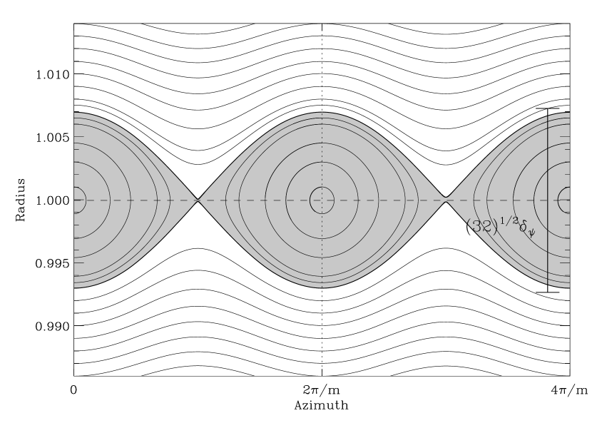
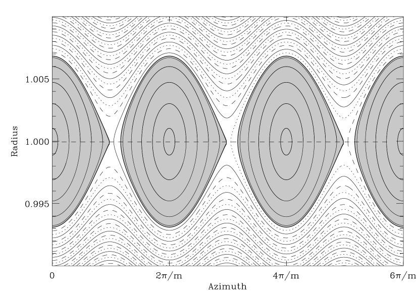
Figure 3: Topology of the streamlines in the inviscid case (left panel) and for the viscous case (right panel). In the right panel, the solid, dotted and dashed lines represent three distinct unique streamlines that show how a fluid element originating in the outer disk eventually reaches the inner disk after passing through the corotation radius between the libration islands. This flow topology is very similar to the one of the horseshoe region in a viscous disk (Masset 2001, 2002).

In Figure 3 we plot the streamlines (from the calculation with highest radial resolution) in the inviscid case and in the viscous case. As we consider a thin disk, for which the pressure length-scale is of the order of the libration scale, the radial width of the libration islands is satisfactorily accounted for by the ballistic expression of equation (2).

We have performed additional calculations for the isolated corotation resonance case in order to investigate whether the viscosity prescription ($\nu=\mbox{constant}$ or $\nu\propto\Sigma^{-2/3}$, as used in the analysis of Ogilvie & Lubow 2003), and the boundary condition prescription, could significantly alter the value and saturation properties of the corotation torque.

The results are shown in Figure 4. The curves with diamonds show the results with a constant viscosity, while the curves with squares show the results with the viscosity prescription $\nu\propto\Sigma^{-2/3}$. All these calculations have $W/\Delta r=21.5$ or $22$. The solid lines show calculations with an inner boundary at $R_{\rm min}=0.88$ and an outer boundary at $R_{\rm max}=1.12$, with damping boundary conditions on the $7$% inner and outer parts of the mesh. The dotted lines show calculations with the same boundary conditions but with an inner boundary at $R_{\rm min}=0.83$ and an outer boundary at $R_{\rm max}=1.17$. Finally the dashed lines show calculations with boundary conditions adapted to the evanescent waves. The dashed and dotted lines strictly have all same parameters, and differ only by their boundary conditions. One can make the following comments:

• There is a systematic offset between a uniform viscosity prescription and the $\nu\propto\Sigma^{-2/3}$ prescription, which amounts to a bit less than 10%, the latter prescription leading to a more saturated resonance.

• The calculation that one would expect to best fit the analytical results of Ogilvie & Lubow (2003) is the one with adapted boundary conditions and a $\nu\propto\Sigma^{-2/3}$ prescription. This corresponds to the dashed line with squares. Although it satisfactorily agrees with the theoretical expectations for $p\leq 0.3$, it leads to a resonance that is less saturated than expected for larger values of $p$. For $p=2.0$, the measured dimensionless torque is offset of $0.1$ from its analytical estimate. Such an offset is unlikely to be due to numerical diffusion, as can be seen in Fig. 2.

• Damping boundary conditions have a small but measurable impact on the fully unsaturated torque value. This might be linked to the fact that with the radially extended mesh that we consider, the boundaries lie within $\sim 2$ driving lengths from the Lindblad resonances. In any case, whenever we shall study a situation with two resonances (either two corotation resonances or one corotation resonance and one Lindblad resonance), we will compare our results to the isolated corotation resonance case by performing separately an isolated resonance test calculation, with exactly the same boundary location and prescription.

4 Saturation of a pair of corotation resonances

We have performed a first set of calculations in which we consider the $m=3$ corotation resonance presented at length in the previous section ($\psi=10^{-5}$, $\Omega=1$), and a second resonance, with potential amplitude $\psi^{\prime}=1.3\cdot 10^{-5}$, with azimuthal wavenumber $m^{\prime}=2$, and with frequency $\Omega^{\prime}$ such that the corotation radius is located at $r=1+s\cdot 10^{-4}$, where $s$ takes the following values: $25,50,100,200,300,500$. With the largest separation ($s=500$), the resonances are well apart and their distance in radius amounts to slightly more than $3$ times the sum of their half-widths, while for the smallest separation, the distance between the corotation radii amounts to only 16% of the sum of their half-widths, so the resonances strongly overlap. For each two-resonance calculation, two other separate calculations with exactly the same parameters are performed, in which one only of the resonances is present. We have performed all these calculations with three different values for the viscosity (chosen here as uniform): $\nu=10^{-6}$, $\nu=10^{-7}$ and $\nu=0$. The first choice corresponds to a low value of the $p$ parameter, and to resonances that are therefore almost unsaturated, while the second choice corresponds to values of $p$ that are close to unity ($p=0.844$ for the $m=3$ resonance, and $p=O(1)$ for the $m^{\prime}=2$ resonance as well, with an exact value that depends on $s$). The mesh parameters were $R_{\rm min}=0.87$, $R_{\rm max}=1.18$, $N_{r}=270$, $N_{\phi}=90$.

4.1 High viscosity

In Figure 5 we show results for four values of the separation ($s=300,100,50,25$) of the highly viscous case. On these plots the variable $\delta$ represents the distance between the corotation radii of the two resonances, $w_{1}$ is the $m=3$ resonance width, and $w_{2}$ is the $m^{\prime}=2$ resonance width, estimated with the ballistic approximation of equation (2). The resonances should overlap when the parameter $\overline{\delta}=2\delta/(w_{1}+w_{2})$ becomes smaller than unity, i.e. when the distance between the corotation radii is smaller than the sum of the resonances’ half-widths.

The variable $\tau_{\rm beat}$ features in Figure 5. It represents the amount of time that separates identical configurations of potential components:

$$\tau_{\rm beat}=2\pi\left|\frac{m^{-1}-m^{\prime-1}}{\Omega-\Omega^{\prime}}\right|$$ (4)

When the two resonances overlap, a passive scalar advected by the flow displays a highly time-dependent behavior, and remarkably, in this highly viscous case, this has no impact on the torque value. The two-resonance torque value is almost insensitive to the resonance overlap, and exhibits a value that is nearly constant in time, whatever the value of $\overline{\delta}$. A tentative explanation for this property could be the following: Ogilvie & Lubow (2003) have emphasized that the nonlinear effect on the corotation torque of an isolated resonance can be understood as the feedback of the perturbation on the vortensity gradient of the disk, and this is likely generalizable to a set of corotation resonances. For a viscosity large enough that the viscous timescale across the libration islands be shorter than any other timescale (libration timescale or beating timescale), the vortensity gradient across the resonances is hardly modified with respect to its unperturbed value, hence nonlinear effects should be negligible and the torque value should be the sum of the linear estimates for each resonance.

4.2 Moderate viscosity

In Figure 6 we show results for six values of the separation ($s=500,300,200,100,50,25$) of the moderately viscous case. On these curves one can see that the two-resonance torque is nearly equal to the sum of the one-resonance torques when the resonances are separated ($\overline{\delta}>1$), although there exists a small but noticeable difference between these two values that increases as $\overline{\delta}$ gets close to unity. When both resonances overlap (bottom panels), the time-averaged two-resonance torque value can be either larger (in absolute value, for $\overline{\delta}=0.63$) or smaller (for $\overline{\delta}=0.32$ or $\overline{\delta}=0.16$) than the sum of the one-resonance torque values. One can also notice a torque modulation with period $\tau_{\rm beat}$. The findings of the highly viscous case therefore do not hold, even for the time-averaged values. Note that $\tau_{\rm beat}$ is only the shortest period over which one can expect the torque modulation to occur, while the longest is $2\pi/[\mbox{GCD}(m,m^{\prime})|\Omega-\Omega^{\prime}|]$, where $\mbox{GCD}(m,m^{\prime})$ is the greatest common divisor of $m$ and $m^{\prime}$, which is $1$ in the case where $|m^{\prime}-m|=1$.

4.3 Inviscid case

In Figure 7 we show results for six values of the separation ($s=500,300,200,100,50,25$) of the inviscid case. Again the solid and dashed-dotted curves are almost indistinguishable by eye when the resonances do not overlap ($\overline{\delta}>1$, corresponding to the top panels), while they are markedly different when they overlap ($\overline{\delta}<1$, bottom panels). All curves slowly decay in absolute value. This is normal for the one-resonance torques and their sum, as the corotation torque in that case tends to saturate, and it is reasonable to expect it also to saturate, on the average, in the two-resonance case. A quasi-periodic torque modulation is apparent for the closest case (right-bottom plot), with a pseudo-period that corresponds to $2\tau_{\rm beat}$.

4.4 Systematic exploration

We have performed calculations similar to the illustrative cases of two corotation resonances of the previous paragraphs, with a more systematic exploration of the (separation, saturation) parameter space. Our aim is to check the following trends:

1. The two-resonance torque value is the sum of the one-resonance torques, whenever the viscosity is high or the resonances do not overlap.

2. The two-resonance torque value of overlapping resonances saturates at low viscosities, in a fashion that is similar to the saturation of a one-resonance torque.

3. The time-averaged torque value of two overlapping resonances for a small or moderate viscosity may sensibly differ from the sum of the isolated resonances torques, but it never exceeds the sum of the fully unsaturated isolated resonance torques.

We therefore set up the following series of calculations:

• We consider two fixed corotation resonances, with frequencies and azimuthal wavenumbers respectively $\Omega=1.015$ and $m=3$, and $\Omega^{\prime}=0.985$ and $m^{\prime}=2$. These resonances have the same forcing potential amplitude $\psi$, which we vary. The disk still has $H/r=0.01$, the mesh has $N_{r}=240$ by $N_{\phi}=90$ zones, the inner mesh boundary is at $R_{\rm min}=0.84$, the outer mesh boundary is at $R_{\rm max}=1.16$. The potential is turned on on the time-scale $\tau=20\;\Omega^{-1}$. We use damping boundary conditions.

• The amplitude of the forcing potential is chosen such that the parameter ${\overline{\delta}}^{-1}=(w_{1}+w_{2})/2\delta$ takes the following values: $0.3$, $0.45$, $0.6$, $0.8$, $1.0$, $1.15$, $1.3$, $1.45$, $1.8$, $2.1$, $2.5$, $2.75$, $3.0$, $4.0$, $5.0$, $6.0$, i.e. from well separated resonances to strongly overlapping resonances. In the above expression $w_{1}$ and $w_{2}$ are evaluated as if the resonance frequencies were both $\Omega=1$, therefore $w_{1}=w_{2}$ since the libration island width, in the ballistic approximation, does not depend on $m$.

• The viscosity is varied such that the saturation parameter, given by equation (3), of the “mean” fictitious resonance that would have $\Omega=1$, the same forcing potential as the two resonances considered, and $m=2.5$, would take the values $p=0.2,0.4,0.6,\ldots 2.0$.

• Each calculation is performed over a time that is larger than the libration time of each resonance, the beating time between them, and the viscous time across each libration zone. The torque is then measured and averaged over the last beating time.

• The same procedure is repeated for two other calculations in which only one of the resonances is present, and which is performed over exactly the same time, and again the torque is measured and time-averaged over the same temporal window (although the beating time is then meaningless). The whole calculation therefore amounts in total to $3\times 16\times 10=480$ such runs.

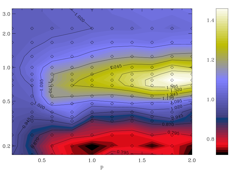
Figure 8: Ratio of the two-resonance torque to the sum of the torque of the corresponding resonances considered separately, as a function of the saturation parameter $p$ and the overlap parameter. Viscosity increases to the left, and the separation increases to the top.

In Figure 8 we plot the ratio of the time-averaged two-resonance torque to the sum the one-resonance torques, as a function of viscosity and resonance separation. As expected, the result is very close to unity near the top and left axes, which respectively correspond to the well separated case and the highly viscous case. This confirms the expectation 1 above.

The fact that the ratio plotted in Figure 8 does not differ from unity by more than roughly $40$% confirms the expectation 2 above, i.e. the saturation curve of total torque vs. $p$, taken at any given value for the overlap parameter, does not significantly differ from the sum of the saturation curves of the corresponding resonances, considered as isolated.

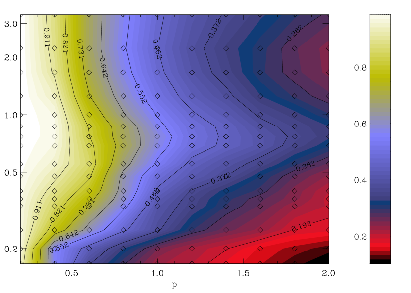
Figure 9: Ratio of the two-resonance torque to the sum of the torques of the corresponding fully unsaturated resonances considered separately, as a function of the saturation parameter $p$ and the overlap parameter. Viscosity increases to the left, and the separation increases to the top.

We plot in Figure 9 the ratio of the two-resonance torque value to the sum of the fully unsaturated torque values of both resonances, as a function of viscosity and resonance separation. This ratio can be seen to never exceed unity, which confirms expectation 3 above.

5 Saturation of a corotation resonance overlapping a Lindblad resonance

As the first-order corotation resonances lie on top of principal Lindblad resonances, we have addressed the restricted problem of the saturation of one corotation resonance that exactly overlaps a Lindblad resonance. We have examined the consequences of this overlap in two different situations:

• The Lindblad torque is small enough so that it does not significantly affect the azimuthally averaged radial profile of surface density. This allows us to compare directly the corotation torque value with its value in the case no Lindblad resonance is present.

• The Lindblad torque is large and significantly redistribute the disk material and thus it considerably alters the slope of vortensity across the resonance. In that case, a direct comparison with a single corotation calculation is not possible. Rather, we measure the slope of vortensity across the resonance and compare the value of the unsaturated resonance to the Goldreich & Tremaine estimate.

5.1 Small Lindblad torque

We consider a corotation resonance excited by a potential with wavenumber $m=3$, frequency $\Omega=1$ and amplitude $\psi=2\cdot 10^{-6}$, which has exactly the same location as a Lindblad resonance excited by a potential with wavenumber $m^{\prime}=2$, frequency $\Omega^{\prime}=3/2$ and amplitude $\psi^{\prime}=5\cdot 10^{-5}$. For the case of an eccentric planet, this corresponds to a slow first-order corotation resonance overlapping a principal outer Lindblad resonance. The reason why we consider such a low-amplitude forcing potential for the corotation resonance is that we wish the onset of possible non-linear effects between the corotation and Lindblad resonances to be as low as possible.

Our mesh extends from $R_{\rm min}=0.84$ to $R_{\rm max}=1.16$, its resolution is $N_{r}=1000$ by $N_{\phi}=90$. The radial resolution is large in order to have a satisfactory resolution of the narrow libration islands of the corotation resonance. The potentials are turned on over the time-scale $\tau=150\;\Omega^{-1}$.

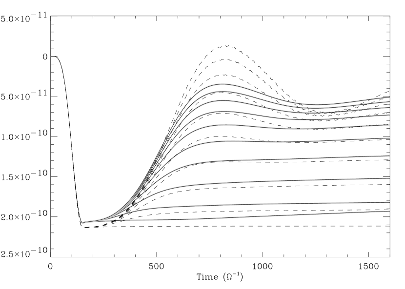
Figure 10: Corotation torque of the resonance described in text, as a function a time, for different values of the viscosity (low viscosities are at the top), for the case of an overlapping Lindblad resonance (solid curves) and for the case of an isolated resonance (dashed curves).

In Figure 10 we plot the torque value of the corotation resonance as a function of time for different values of the viscosity, corresponding to an arithmetic sequence of the saturation parameter $p$, for a mixed corotation/Lindblad resonance and for the case of an isolated corotation resonance with the same characteristics.

Both series of curves exhibit very similar trends. The torque of the isolated resonance tends to oscillate more than the one overlapping a Lindblad resonance, at low viscosity. One can also notice the very long libration time, due to the narrowness of the libration islands.

In Figure 11 we plot the dimensionless torque as a function of the saturation parameter, obtained from the time average of the torque values presented in Figure 10, over the interval $800\;\Omega^{-1}<t<1600\;\Omega^{-1}$.

The time-averaged torque estimate at low viscosity, especially for the isolated resonance, may be slightly biased by the fact that it has not enough time to reach a steady saturation level over the full duration of the calculation. The impact of this bias is however small, and the conclusion that can be drawn from the examination of Figure 11 is that the torque saturation properties are hardly affected by the presence of the underlying Lindblad resonance. The tiny difference between both curves can be attributed either to the relatively small number of libration times over which the time average is performed (at low viscosity) or to the slight radial redistribution of the disk material under the action of the Lindblad torque. The tiny change of the vortensity slope, defined as $-d\log(\Sigma/B)/d\log r$ (where $B$ is the second Oort’s constant), can indeed be estimated to be of the order of a few percent, compatible with the discrepancy of the two saturation curves.

5.2 Large Lindblad torque

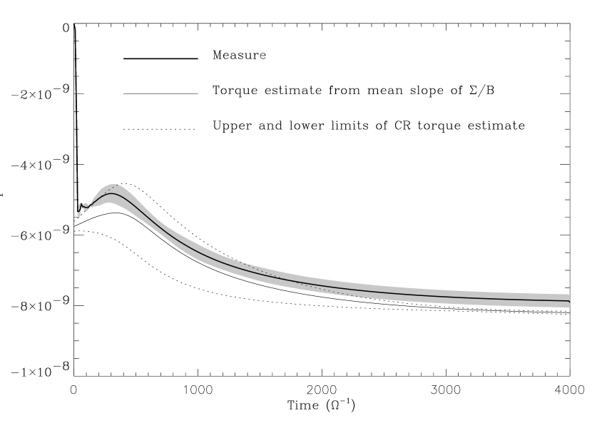
Figure 12: Torque of a corotation resonance overlapping a Lindblad resonance (thick solid line). The Goldreich & Tremaine estimate of that torque using the mean value of the slope of $\Sigma/B$ across the corotation resonance width is shown with the thin solid line, while the extreme values of this estimate, which correspond to the extrema of the slope of $\Sigma/B$ across the resonance width, are shown as dotted lines. The shaded area corresponds to the excursion of the torque value, which is modulated on the short time-scale $\tau_{\rm beat}$. The right panel shows the vortensity profile at $t=0$ (tilted dotted line) and at $t=2000\;\Omega^{-1}$. The common position of the resonances is marked with the dashed line. The equidistant vertical dotted lines show the limit of the corotation libration islands – determined as if it was isolated.

We have also performed a test calculation in which the forcing potential amplitude of the Lindblad resonance is much larger, so that it modifies the surface density profile, in a reduced version of what occurs at a gap edge. We cannot vary the viscosity in this kind of calculation, as we want the surface density profile to converge toward the redistributed profile in a reasonable amount of time. At viscosities low enough to significantly saturate the corotation torque, the viscous time-scale across the excavated region becomes prohibitively large. We therefore just compare the corotation torque value to the Goldreich & Tremaine estimate, obtained by measuring the slope of $\Sigma/B$ across the resonance width at any instant in time. In Figure 12, the left panel shows the comparison between this estimate and the actual corotation torque value. They agree to within a few percent, and the actual torque value is slightly smaller than the Goldreich–Tremaine estimate. The parameters that we adopted for this calculation are:

• $\psi=10^{-5}$, $m=3$ and $\Omega=1$ for the corotation resonance,

• $\psi^{\prime}=10^{-4}$, $m^{\prime}=2$ and $\Omega^{\prime}=1/2$ for the Lindblad resonance. This frequency implies that it is an ILR. If we wanted to strictly reproduce the overlap between a first-order corotation resonance and a principal inner Lindblad resonance, we should have $m_{\rm ILR}=m_{\rm CR}+1$. We have chosen instead $m_{\rm ILR}=m_{\rm CR}-1$, which allows us to better resolve the wave launched at the Lindblad resonance for a given value of $N_{\phi}$. We anticipate that our conclusions are not affected by this choice.

6 Low-resolution issues

The above sections essentially validate the previous work of Ogilvie & Lubow (2003) on the saturation of an isolated corotation resonance, in the context of the first-order corotation resonances of an eccentric giant planet, which are not isolated. The numerical simulations performed thus far on the problem of the eccentricity excitation of a giant planet did not exhibit any eccentricity growth for Jupiter-sized giant planets (Papaloizou et al. 2001). While there may be a number of reasons for that, we show in this section how the corotation torque estimate is mangled at very low resolution, i.e. when the width of the libration islands is of the order of the mesh radial size. The width of a first-order corotation resonance is given by:

$$\frac{W}{r}\approx 4.1(C_{m}^{\pm}meq)^{1/2},$$ (5)

where $q$ is the mass ratio and $C_{m}^{\pm}$ is a factor of order unity given in Tables 1 and 2 of Ogilvie & Lubow (2003). Assuming one has a Jupiter-sized planet orbiting a solar mass star ($q=10^{-3}$) with eccentricity $e=0.01$, the resonance width is therefore $W/r\approx 0.013(C_{m}^{\pm}m)^{1/2}$. As a point of comparison, in run N1 in Papaloizou et al. (2001), which corresponds to a Jupiter-sized giant planet, the radial resolution is $\Delta r/r=0.043$.

Figure 13 shows the results (as before, diamonds are for a uniform viscosity prescription while squares are for a $\nu\propto\Sigma^{-2/3}$ viscosity prescription). The solid lines are for a resolution $W/\Delta r=1.0$, the dotted one $W/\Delta r=0.5$ and the dashed one $W/\Delta r=2.0$. This shows again that the value of the fully unsaturated corotation torque is relatively well reproduced even at very low resolution, but the saturated resonant torque is completely mangled at low resolution. The case $W=\Delta r$ is particularly striking, since in this case one gets a torque value larger than the Goldreich & Tremaine estimate. Therefore in a low-resolution simulation of an embedded giant planet, as soon as the eccentricity gets to values which give the libration islands a size comparable to the radial resolution, these effects could lead to a strong spurious damping of the eccentricity, which would therefore be bounded by small values ($O[0.01]$, depending on the resolution).

7 Conclusions

By means of reduced two-dimensional numerical simulations, involving two resonances at the same time and each resonance separately in order to compare the isolated case to the two-resonance case, we reach the following conclusions:

• The corotation torque of two overlapping resonances coincides with the sum of the corotation torques of each resonance, considered as isolated, either when the resonances do not overlap (their separation is larger than the sum of the half-widths of their libration islands) or when the viscosity is large (fully unsaturated resonances).

• When the resonances overlap and are partially saturated, the two-resonance torque may differ at most by a few tens of percent from the sum of the isolated torques, evaluated for the same viscosity. This implies that a given degree of saturation of a non-isolated resonance is reached for a value of the viscosity of the same order of magnitude as the viscosity needed to achieve the same degree of saturation for the isolated resonance.

• The time-averaged two-resonance torque never exceeds the sum of the Goldreich & Tremaine estimates of each resonance.

• In the case where a corotation resonance overlaps a weak Lindblad resonance (that does not significantly redistribute the vortensity profile), the time-averaged torque value differs from the isolated case by at most a few percent, whatever the value of the viscosity.

• In the case where a corotation resonance overlaps a strong Lindblad resonance, for which our calculations are limited to high-viscosity situations, the time-averaged torque value corresponds to the Goldreich & Tremaine estimate, i.e. to the torque of the unsaturated corotation resonance, considered as isolated.

• The only case in which we have observed a corotation torque value that is larger than the Goldreich & Tremaine estimate (which therefore jeopardizes an eccentricity excitation for the set of parameters quoted in the introduction) is when the mesh resolution is too low. This is therefore a numerical artifact, and we conclude that a high resolution is needed in the region of first-order corotation resonance (i.e. close to the gap edges) in order to observe an eccentricity excitation, with libration islands spanning at least about $10$ zones radially.

Finally, we emphasize that the saturation of the first-order corotation resonances is only one of the factors determining whether the eccentricity of a giant protoplanet grows or decays through its interaction with the disk. An aspect of this problem that tends to be overlooked is the secular exchange of eccentricity between the planet and the disk, which may occur on a time-scale of thousands of orbital periods. The mechanism responsible for this exchange is sometimes referred to as the apsidal resonance (Goldreich & Sari 2003), although this resonance is so broad in a nearly Keplerian disk that we prefer to avoid this denomination. When a planet is placed on an elliptical orbit in a circular disk, its eccentricity should initially decrease as eccentricity is imparted to the disk. This exchange can, in principle, occur in a way that conserves the angular momentum deficit of the coupled disk–planet system, in which case the eccentricity of the planet will be restored later in the cycle of secular exchange. Therefore, a transient decrease of the planet’s eccentricity in such circumstances should not be confused with eccentricity damping. In the analogous problem of the secular inclination dynamics of coupled disk–planet systems, Lubow & Ogilvie (2001) have defined a positive-definite measure of the bending disturbance of the system, equivalent to an angular momentum deficit, which is conserved in the secular exchange and evolves only through the effects of mean-motion resonances and viscous damping. Papaloizou (2002) has also treated aspects of the eccentricity dynamics of coupled disk–planet systems, while Ogilvie (2001) has drawn attention to the subtle issue of whether eccentricity is damped or excited by viscous or turbulent stresses in the disk, and at what rate.

A fully self-consistent calculation therefore involves many additional complications, such as the treatment of the force arising from the material inside of the Roche lobe, the role of self-gravity, and the eccentric coupling between the disk and the planet through the apsidal waves. It will be presented in a forthcoming work.

Table 1: List of the locations of resonances and their action on the eccentricity. Bracketed terms correspond to co-orbital resonances ($\Omega=\Omega_{p}$) which play no role when the planet clears a gap.

Resonance	$(\frac{r}{r_{p}})^{-2/3}=\frac{\Omega}{\Omega_{p}}$	$(\frac{1}{e})(\frac{de}{dt})_{\rm res}$
Principal OLR	$\frac{m}{m+1}$	$+$
Principal ILR	$\frac{m}{m-1}$	$-$
Principal CR	$1$	$[?]$
Fast first-order OLR	1	$[-]$
Fast first-order ILR	$\frac{m+1}{m-1}$	$+$
Fast first-order CR	$\frac{m+1}{m}$	$-$
Slow first-order OLR	$\frac{m-1}{m+1}$	$+$
Slow first-order ILR	$1$	$[-]$
Slow first-order CR	$\frac{m-1}{m}$	$-$

Figure 1: Corotation torque exerted by the external potential on the disk as a function of time, for an inviscid disk (upper curves) or for a viscous disk (lower curves), for different radial resolutions. The curves corresponding to the viscous case differ very little from each other, as can be seen in the close-up.

Figure 2: Dimensionless residual corotation torque as a function of resolution, for an inviscid disk.

Figure 4: Dimensionless corotation torque value of an isolated $m=3$ resonance, as a function of the saturation parameter. The thick solid line shows the theoretical curve for the case $\nu\propto\Sigma^{-2/3}$ (Ogilvie & Lubow 2003).

Figure 5: Corotation torque of a pair of corotation resonances (solid line) in the high-viscosity case, as a function of time. The dotted line shows the corotation torque of the isolated $m=3$ resonance, which is the same on all plots since this resonance is fixed. The dashed line shows the corotation torque of the isolated $m^{\prime}=2$ resonance, and the dot-dashed line the sum of these one-resonance corotation torques. On the first two plots, this curve and the solid curve are indistinguishable by eye, while a slight offset can be noticed in the strongly overlapping cases (bottom plots). It can be noticed that the two-resonance corotation torque adopts an almost constant value over a time that is larger than $\tau_{\rm beat}$. One can note a fast oscillation of the torque value with a small amplitude. These oscillations are found on the two-resonance runs as well as on the isolated $m^{\prime}=2$ runs, so they are probably due to the fact that the $m^{\prime}=2$ potential component and the mesh do not corotate.

Figure 6: Corotation torque of a pair of corotation resonances in the moderate-viscosity case, as a function of time. The curve styles are the same as in the previous figure.

Figure 7: Corotation torque of a pair of corotation resonances in the inviscid case, as a function of time. The curve styles are the same as in the previous figure.

Figure 11: Dimensionless corotation torque as a function of the saturation parameter $p$, for the case of a mixed corotation/Lindblad resonance (solid line) and for the case of an isolated corotation resonance (dashed line).

Figure 13: Dimensionless torque of an isolated corotation resonance as a function of viscosity, for three different resolutions.

References

- (1) d’Angelo, G., Kley, W., & Henning, T. 2003, ApJ, 586, 540
- (2) Bate, M. R., Lubow, S. H., Ogilvie, G. I., & Miller, K. A. 2003, MNRAS, 341, 213
- (3) Ford, E. B., Havlickova, M., & Rasio, F. A. 2001, Icarus, 150, 303
- (4) Goldreich, P. & Sari, R. 2003, ApJ, 585, 1024
- (5) Goldreich, P. & Tremaine, S. 1979, ApJ, 233, 857
- (6) Goldreich, P. & Tremaine, S. 1980, ApJ, 241, 425
- (7) Holman, M., Touma, J., & Tremaine, S. 1997, Nature, 386, 254
- (8) Kley, W. 1998, A&A, 338, 37
- (9) Lubow, S. H. & Ogilvie, G. I. 2001, ApJ, 560, 997
- (10) Masset, F. S. 2002, A&A, 387, 605
- (11) Masset, F. S. 2001, ApJ, 558, 453
- (12) Masset, F. S. 2000a, A&AS, 141, 165
- (13) Mazeh, T., Krymolowski, Y., & Rosenfeld, G. 1997, ApJ, 477, L103
- (14) Meyer-Vernet, N. & Sicardy, B. 1987, Icarus, 69, 157
- (15) Nelson, R. P., Papaloizou, J. C. B., Masset, F. S., & Kley, W. 2000, MNRAS, 318, 18
- (16) Ogilvie, G. I. 2001, MNRAS, 325, 231
- (17) Ogilvie, G. I. & Lubow, S. H. 2003, ApJ, 587, 398
- (18) Papaloizou, J. C. B. 2002, A&A, 388, 615
- (19) Papaloizou, J. C. B., Nelson, R. P., & Masset, F. S. 2001, A&A, 366, 263
- (20) Rasio, F. A. & Ford, E. B. 1996, Science, 274, 954
- (21) Stone, J. M. & Norman, M. L. 1992, ApJS, 80, 753
- (22) van Leer, B. 1977, Journal of Computational Physics, 23, 276