Dynamical Mass Estimates for Five Young Massive Stellar Clusters

Abstract

We have obtained high-dispersion spectra for four massive star clusters in the dwarf irregular galaxies NGC 4214 and NGC 4449, using the HIRES spectrograph on the Keck I telescope. Combining the velocity dispersions of the clusters with structural parameters and photometry from images taken with the Hubble Space Telescope, we estimate mass-to-light ratios and compare these with simple stellar population (SSP) models in order to constrain the stellar mass functions (MFs) of the clusters. For all clusters we find mass-to-light ratios which are similar to or slightly higher than for a Kroupa MF, and thereby rule out any MF which is deficient in low-mass stars compared to a Kroupa-type MF. The four clusters have virial masses ranging between $2.1\times 10^{5}\mbox{$M_{\odot}$}$ and $1.5\times 10^{6}\mbox{$M_{\odot}$}$, half-light radii between 3.0 and 5.2 pc, estimated core densities in the range $2\times 10^{3}\,\mbox{$M_{\odot}$}\,{\rm pc}^{-3}$ to $2\times 10^{5}\,\mbox{$M_{\odot}$}\,{\rm pc}^{-3}$ and ages between 200 Myr and 800 Myr. We also present new high-dispersion near-infrared spectroscopy for a luminous young ($\sim 15$ Myr) cluster in the nearby spiral galaxy NGC 6946, which we have previously observed with HIRES. The new measurements in the infrared agree well with previous estimates of the velocity dispersion for this cluster, yielding a mass of about $1.7\times 10^{6}\mbox{$M_{\odot}$}$. The properties of the clusters studied here are all consistent with the clusters being young versions of the old globular clusters found around all major galaxies.

1 Introduction

The term “super star cluster” was probably first coined by van den Bergh (1971), who used it to describe a number of highly luminous, compact sources in the starburst in M 82. Similar clusters have since been found in many other galaxies, often (but not exclusively) in starbursts and mergers. Thanks to high resolution imaging with the Hubble Space Telescope, it is now clear that these clusters in many ways resemble young versions of the classical (old) globular clusters found around all large galaxies. This, in turn, has fuelled expectations that these objects may provide an opportunity to gain first-hand insight into the formation mechanisms and early evolution of globular clusters.

One question which has spawned considerable debate concerns the stellar initial mass function (IMF) of young star clusters, and whether or not variations exist. Such variations might have implications for cluster survival, since clusters with a shallow IMF are more easily disrupted (Goodwin, 1997) and may not be able to survive for a Hubble time. By definition the initial mass function can only be observed at the time of formation. Observations of older clusters (or stellar populations in general) reveal a present-day mass function (MF) which may be different from the initial one. At the high-mass end, the two will differ because of stellar evolution, but in a stellar cluster there can also be differences between the IMF and the present-day MF at the low-mass end due to effects of dynamical evolution. Thus, we will deliberately omit the I in the term IMF throughout this paper.

Even with the HST, direct observations of all but the brightest individual stars in extragalactic star clusters are generally impossible, so attempts to constrain the MF have to rely on indirect methods. One approach which has gained popularity in recent years is to combine information about structural parameters for the clusters, typically derived from HST imaging, with velocity dispersion measurements obtained from integrated-light spectra with high-dispersion spectrographs, and estimate the mass-to-light (M/L) ratios by application of the virial theorem. If the cluster ages are known (for example from broad-band colors), the virial M/L estimates can then be compared with predictions by simple stellar population (SSP) models computed for various MFs. Ho & Filippenko (1996a, b) studied three young clusters in the two nearby dwarf galaxies NGC 1569 and NGC 1705 and found masses of several times $10^{5}\,\mbox{$M_{\odot}$}$. Analyzing the same data and comparing with SSP models, Sternberg (1998) found some evidence for variations in the MF slope between the three clusters. Several other recent studies have reported a mixture of “normal” (usually meaning Kroupa 2002 or Salpeter 1955-like) and top-heavy MFs (Smith & Gallagher, 2001; Mengel et al., 2003; Maraston et al., 2003; Gilbert & Graham, 2003; McCrady et al., 2003). While in principle straight-forward, the simple application of the virial theorem is in practice complicated by several factors, such as the assumption of virial equilibrium (which may not be valid for the youngest clusters) and isotropy of the velocity distribution, mass segregation (primordial or as a result of dynamical evolution), presence of binary stars, and (especially for more distant systems) crowding- and resolution effects. Evidence for a top-heavy MF has also been claimed based on Balmer line strengths measured on medium-resolution spectra for clusters in the peculiar galaxy NGC 1275 (Brodie et al., 1998).

In this paper we report new observations of four luminous young star clusters in the two nearby irregular dwarf galaxies NGC 4214 and NGC 4449. HST photometry for the clusters has been published by Billett et al. (2002, hereafter BHE02) and Gelatt et al. (2001, GHG01). A primary selection criterion for our spectroscopic follow-up was that the clusters be isolated and appear on as uniform a background as possible, allowing accurate measurements of their structural parameters and velocity dispersions. In addition, the clusters all have estimated ages greater than 100 Myrs. With typical crossing times of $\sim 10^{6}$ years the assumption of virial equilibrium is expected to be a very plausible one for these clusters. We have obtained high-dispersion spectra with the HIRES spectrograph (Vogt et al., 1994) on the Keck-I telescope and use these spectra to measure velocity dispersions for the clusters. We have also observed a younger cluster in the nearby spiral galaxy NGC 6946 with the NIRSPEC spectrograph on the Keck-II telescope. We have previously observed this cluster with HIRES (Larsen et al., 2001, hereafter LAR01), so the new data provide a welcome consistency check of our earlier results.

For the distances to NGC 4449 and NGC 6946 we assume 3.9 Mpc and 6.0 Mpc (Gelatt et al., 2001; Karachentsev et al., 2000). The distance to NGC 4214 has long been assumed to be around 4–6 Mpc and BHE02 used 4.8 Mpc. However, recent measurements by Drozdovsky et al. (2002) and Maíz-Apellániz et al. (2002) based on HST photometry of the red giant branch suggest significantly smaller values of $2.7\pm 0.3$ Mpc and $2.94\pm 0.18$ Mpc, respectively. Here we adopt a compromise of $2.8\pm 0.3$ Mpc.

2 Observations and data reduction

2.1 WFPC2 imaging

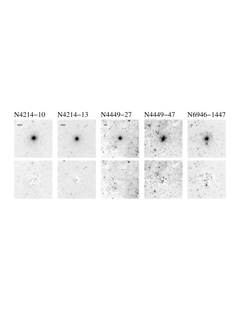
Figure 1: HST F555W images of the five clusters. Each top panel shows a $6\arcsec\times 6\arcsec$ section of the image centered on the cluster. The bar in the upper left corner of each panel indicates a linear scale of 10 pc. The bottom panels show the residuals after subtraction of the best-fitting EFF model convolved with the TinyTim PSF.

Table 1 lists the cluster IDs and the HST datasets used for this analysis. Coordinates for the clusters and discussion of their host galaxy properties can be found in GHG01, BHE02 and LAR01. HST images of the clusters are shown in Fig. 1. When possible, multiple exposures were combined to reject cosmic ray hits, but in many cases we only had a single exposure in each band. The cluster N4214-13 was saturated on the F555W and longer F814W exposures obtained under programme 6569, so for this cluster we used only the F336W data and a single short F814W exposure from that programme. Other images in F606W, F555W and F814W were available for N4214-13 from programmes 5446 and 6716 and these were all used for the analysis. For the two clusters in NGC 4449, only a single exposure in each of the F555W and F814W bands were used. Exposures in F336W were also available for this galaxy from programme 6716 and were used by GHG01 for photometry, but had too low S/N for our size measurements. For the photometry of clusters in NGC 4214, NGC 4449 and NGC 6946 we use the data published in BHE02, GHG01 and Larsen et al. (2001), and we refer to those papers for further details. The colors and $V$ magnitudes, corrected for Galactic foreground extinction, are listed in Table 2. Note that GHG01 and BHE02 also included a correction of $E(B-V)=0.05$ mag for internal reddening in the galaxies, which is included for the photometry in Table 2.

2.2 Ages and reddenings

Cluster ages and reddenings were determined by comparing Bruzual & Charlot (2003, hereafter BC03) model predictions for the evolution of broad-band colors as a function of age for simple stellar populations (SSPs) with the observed cluster colors. We used the BC03 models tabulated for a Salpeter (1955) stellar MF extending down to $0.01\,\mbox{$M_{\odot}$}$, but the exact MF choice is not important for the age determinations because the integrated colors of clusters are dominated by stars in a narrow mass range near and just above the turn-off. The BC03 models are also tabulated for a Chabrier MF, and we verified that using this MF yielded nearly identical results to the Salpeter MF, as expected. The MF choice does of course have a significant impact on the mass-to-light ratios, as will be discussed below.

Fig. 2 shows the BC03 model sequence in the ($U-V$, $V-I$) plane for metallicity $Z=0.008$ and the five datapoints corresponding to the cluster photometry in Table 2 (without any additional reddening corrections). Ages are indicated along the sequence. The arrow indicates the reddening vector for $A_{B}=1$ mag, according to the Galactic extinction law in Cardelli et al. (1989). Ages and reddenings were determined for each cluster by projecting the observed colors along the reddening vector until the best match to the BC03 models was obtained. We have only two colors for 4 of the 5 clusters and for these objects the best match between model and observed colors simply corresponds to the intersection between a line drawn through the datapoints in Fig. 2 along the reddening vector and the model sequence. For NGC6946-1447 more colors are available and an exact match to the model colors can not be achieved. For this cluster we selected the age/reddening combination corresponding to the closest match between the projection of the observed colors along the reddening vector and the BC03 models.

The best fitting age- and extinction estimates are given for $Z=0.004$, $Z=0.008$ and $Z=0.02$ (solar) models in Table 2. While the metallicities of the clusters themselves are unknown, estimates of oxygen abundances for Hii regions in NGC 4214 and NGC 4449 are available in the literature. For two knots in NGC 4214, Kobulnicky & Skillman (1996) found 12 + $\log$(O/H) = $8.173^{+0.020}_{-0.022}$ and $8.267^{+0.015}_{-0.017}$, corresponding to [O/H]$\sim-0.57$ (taking the Solar [O/H] from Lang (1997)). For NGC 4449, Lequeux et al. (1979) measured 12 $+$ $\log$(O/H) = 8.3 or [O/H]$=-0.49$. Assuming solar-scaled abundances, these Oxygen abundances correspond to $Z=0.0054$ and $Z=0.0065$, intermediate between the BC03 $Z=0.004$ and $Z=0.008$ models. The [O/H] abundance in NGC 6946 was estimated for two clusters near N6946-1447 by Efremov et al. (2002), who found 12 $+$ $\log$(O/H) = 8.95$\pm$0.2, consistent with the Solar value. Since the $Z=0.004$ models give a negative reddening for N4449-27 (even accounting for the $E(B-V)=0.05$ internal reddening correction implicit in the photometry) and the ages and reddenings derived for NGC 4214 are nearly independent of the assumed metallicity, we will use the age and metallicity estimates derived for $Z=0.008$ for the clusters in NGC 4214 and NGC 4449 and those derived for $Z=0.020$ for the cluster in NGC 6946. The age estimates are then virtually identical to those tabulated by BHE02 and GHG01, who used Starburst99 models. For N6946-1447, it is interesting to note that the procedure adopted here also yields a very similar age estimate to that obtained by LAR01, where the Girardi et al. (1995) “S”-sequence calibration was used. While the S-sequence method is attractive because of its empirical founding, it is (at least for now) restricted to $UBV$ colors, and the multi-color approach adopted here allows for a more robust estimate of the foreground reddening.

Obtaining realistic estimates of the errors on the derived ages and reddenings is not straight-forward. The errors given in Table 2 are based on the photometric uncertainties only. They were estimated by adding random offsets to the input photometry, drawn from Gaussian distributions with standard deviations corresponding to the photometric errors, and rederiving the ages and metallicities. This procedure was repeated 100 times for each cluster, and the standard deviations of the resulting distributions of age- and metallicity estimates were then taken as estimates of the corresponding 1 $\sigma$ uncertainties. It is clear, however, that systematic uncertainties can dominate over the random errors. Table 2 illustrates the metallicity dependence, but the models themselves are also uncertain. Stellar models from different groups (e.g. Padua vs. Geneva: Girardi et al., 2000; Lejeune & Schaerer, 2001) differ significantly in their predictions for the effective temperature, luminosity and lifetimes of red supergiants, for example, which translates into uncertainties on the integrated colors of simple stellar population models. To avoid artificially low uncertainties on the log(age) estimates for the clusters with very small errors on the photometry, we adopt 0.1 or the values in Table 2, whichever is larger.

2.3 Cluster sizes

For the measurements of cluster sizes we used the ISHAPE profile-fitting code, which has been tested and described in Larsen (1999). Briefly, the code models the image of a cluster by assuming an analytic model for the intrinsic profile and then convolves the model with a user-specified point spread function (PSF). The shape parameters of the model are iteratively adjusted until the best possible match to the data is obtained. A particularly relevant feature for this work is that ISHAPE assigns weights to each pixel by measuring the standard deviation in concentric rings around the center of the object. Pixels which deviate by more than 2$\sigma$ from other pixels in each annulus are assigned zero weight, effectively eliminating pixels affected by cosmic rays from the fitting process.

We assumed cluster profiles of the form

$$P(r)\propto\left[1+(r/r_{c})^{2}\right]^{-\alpha}$$ (1)

These profiles differ from the classical King (1962) models for globular clusters in that they do not have a well-defined tidal radius, but they have been shown by Elson et al. (1987) to provide very good fits to young clusters in the Large Magellanic Cloud. In the following we refer to them as EFF profiles. During the fitting procedure, we allowed both the core radius $r_{c}$ and envelope slope parameter $\alpha$ to vary as free parameters. The input WFPC2 PSFs were constructed using version 6.0 of the TinyTim software including a convolution with the “diffusion kernel” to simulate charge diffusion between neighboring pixels. Separate PSFs were generated for each band at the position of each cluster. The residuals after subtraction of the best-fitting EFF models, convolved with the TinyTim PSF, are shown for the F555W images in the bottom panels of Fig. 1. The intensity scales in the bottom and top panels are identical.

Table 3 summarizes the EFF profile fits for a fitting radius of $3\arcsec$. For each cluster we list the S/N within the fitting radius, followed by the fitted FWHM (in arcsec, corrected for the HST PSF) and envelope slope parameter $\alpha$. The conversion from FWHM and $\alpha$ values to effective (half-light) radii, needed for the virial mass determinations (Sec. 3), depends on the adopted outer radius of the cluster profiles. In the case of infinite cluster size and $\alpha>1$, the effective radius $r_{\rm eff}$ is

$$\mbox{$r_{\rm eff}$}\,=\,r_{c}\,\sqrt{(1/2)^{\frac{1}{1-\alpha}}-1}$$ (2)

where $r_{c}$ is the core radius in Eq. (1), related to the FWHM as

$${\rm FWHM}\,=\,2\,r_{c}\,\sqrt{2^{1/\alpha}-1}.$$ (3)

However, for $\alpha<1$ the total volume contained under the EFF profile is infinite, and $r_{\rm eff}$ therefore undefined. If $\alpha$ is only slightly greater than 1, the $r_{\rm eff}$ computed from Eq. (2) can be very large. Thus, more meaningful estimates of $r_{\rm eff}$ may be obtained by adopting a finite outer radius for the cluster profile:

$$\mbox{$r_{\rm eff}$}\,=\,r_{c}\left[\left\{\frac{1}{2}\left[\left(1+\frac{\mbox{$r_{\rm max}$}^{2}}{r_{c}^{2}}\right)^{1-\alpha}+1\right]\right\}^{\frac{1}{1-\alpha}}-1\right]^{1/2}$$ (4)

where $r_{\rm max}$ is the adopted outer limit of the cluster. In Table 3 we list $r_{\rm eff}$ values for $\mbox{$r_{\rm max}$}=3\arcsec$, $5\arcsec$ and $\mbox{$r_{\rm max}$}=\infty$. While the $r_{\rm eff}$ values do show some dependence on the adopted $r_{\rm max}$, especially for clusters with relatively shallow envelopes (N4214-13, N6946-1447), the difference between $\mbox{$r_{\rm max}$}=3\arcsec$ and $\mbox{$r_{\rm max}$}=5\arcsec$ is comparable to the overall scatter in the measurements on different images. We also carried out fits within a fitting radius of $1\farcs 5$, and found the results to be consistent with the numbers in Table 3 within the uncertainties.

We also carried out a series of King model fits to the cluster profiles, the results of which are listed in Table 4. The King profiles might seem a more obvious choice since they depend on only two parameters, namely the core radius and concentration parameter $c=r_{t}/r_{c}$, where $r_{t}$ is the tidal radius, and there is no need to introduce an artificial cut-off radius. The problem is that $r_{t}$ is often poorly constrained, leading to substantial uncertainties on $r_{\rm eff}$. Nevertheless, the King profile fits in Table 4 are generally consistent with our estimates of the half-light radii from the EFF fits. In the following we use the mean values listed in Table 3 for fitting radius of $3\arcsec$ and $\mbox{$r_{\rm max}$}=3\arcsec$.

2.4 HIRES and NIRSPEC spectroscopy

The four clusters in NGC 4214 and NGC 4449 were observed on May 8 and May 9, 2003, with the HIRES spectrograph on the Keck-I telescope. We used the C2 decker, providing a slit width of $0\farcs 861$ and a resolution of $\lambda/\Delta\lambda=45000$. A spectral range of 5450Å–7800Å was covered, with some gaps between the 20 echelle orders. Integration times were about 3 hours for each object, typically split into 3 exposures. This yielded signal-to-noise (S/N) ratios of 15–55 per pixel in the dispersion direction in the combined spectra. The raw exposures were reduced with the MAKEE package written by T. Barlow and tailored specifically for HIRES spectra. MAKEE automatically performs bias subtraction and flat-fielding, then traces the echelle orders in the input images, extracts the spectra and performs wavelength calibration using observations of calibration lamps mounted within the spectrograph and night sky lines to fine-tune the zero-points. Finally, the spectra were average combined using a sigma-clipping algorithm to eliminate any remaining cosmic-ray hits not recognized by MAKEE.

The cluster in NGC 6946 was observed on Jul 13, 2002 with the NIRSPEC near-infrared spectrograph (McLean et al., 1998) on Keck-II, using a $0\farcs 432$ slit. Observations were obtained for two echelle-mode settings, covering the $H$ and $K$ bands with a spectral resolution of $\lambda/\Delta\lambda=25000$. Integrations were made in pairs of 240 s each, nodded by a few arcsec along the slit to allow sky subtraction. Observations of an A-type star (HR 44) were obtained for removal of telluric lines from the spectra. The data were reduced with the REDSPEC package written by L. Prato, S. S. Kim & I. S. McLean, but with two modifications by us: 1) we modified the extraction algorithm to perform optimal extraction of the spectra (Horne, 1986), and 2) we implemented a cross-correlation technique to fine-tune the wavelength scale of the calibrator spectrum. Finally, the spectra were averaged in the same way as for the HIRES data.

Details of the HIRES and NIRSPEC observations are provided in Table 5. In addition to the cluster spectra, a number of template stars for the velocity dispersion measurements were also observed during both the HIRES and NIRSPEC runs. These are listed in Table 6 and 7. Absolute $M_{V}$ magnitudes are listed for each star, based on Hipparcos parallaxes (Perryman et al., 1997) and the $V$ magnitudes in the Bright Star Catalogue (Hoffleit & Jaschek, 1991). For the HIRES run we observed both giant and supergiant template stars, since the clusters in NGC 4214 and NGC 4449 are sufficiently old that giant stars might be more appropriate templates. For the NIRSPEC run, only the luminosity class (LC) I and II stars were observed.

Velocity dispersions were measured using the cross-correlation technique first described by Tonry & Davis (1979) and applied to young clusters by Ho & Filippenko (1996a, b). We have previously used this method in LAR01 for our analysis of N6946-1447 HIRES data and refer to that paper for details specific to our approach. In brief, the cluster spectra were cross-correlated with the spectra of the template stars, using the FXCOR task in the RV package within IRAF. Prior to the cross-correlation, the spectra were continuum-subtracted using a cubic spline and any remaining large scale variations were eliminated by further applying a high-pass filter cutting at a wavenumber of 10. The FWHM of the peak of the resulting cross-correlation function (CCF) is a measure of the broadening of the stellar lines in the cluster spectrum, here assumed to be mainly due to the line-of-sight velocity dispersion, $v_{x}$. Because the spectra are continuum-subtracted and only the width of the CCF peak is used, addition of a smooth continuum to the spectra (e.g. from early-type stars in the clusters) does not affect the velocity dispersion measurements. In the original implementation of the method described by Tonry & Davis (1979), the $v_{x}$ is determined as the quadrature difference between the Gaussian dispersion of the CCF peak of the template versus object spectra ($\mu$) and the internal velocity dispersion of the template, $\tau$:

$$v_{x}^{2}\,=\,\mu^{2}\,-\,2\tau^{2}$$ (5)

Setting $v_{x}^{2}=0$ for the template spectrum, it is seen that $2\tau^{2}$ is simply the squared dispersion of the CCF peak for two template star spectra. Thus, $v_{x}^{2}$ is the squared difference of the dispersions of the two CCF peaks. A convenient feature of the cross-correlation method is that instrumental resolution effects cancel out, as long as they are the same for the object- and template spectra. In principle this also applies to any intrinsic broadening of the stellar lines, for example by macroturbulent motions in the atmospheres.

If the CCFs do not have a Gaussian shape, it is unclear how to relate the FWHM values output by the FXCOR task to Gaussian sigmas. Thus, we adopted a slightly different approach than simply applying Eq. (5). The relation between the FWHM of the CCF peak and $v_{x}$ was established by convolving the template star spectra with a series of Gaussians corresponding to $v_{x}$ values bracketing the values expected for the clusters, and then cross-correlating the broadened template star spectra with the unbroadened ones. Thus, each cross-correlation product of broadened and un-broadened spectra led to an estimate of the CCF peak FWHM for the corresponding broadening, which could then be compared with the FWHM of the cluster versus template CCF. The cross-correlation method does not rely on any individual, strong lines, but utilizes the multitude of fainter lines from late-type stars that are present in the spectra. In fact, it is better to avoid strong lines like the Ca II triplet where saturation effects set in. For this work, we performed the analysis separately for each echelle order, though not all echelle orders were included. Some orders included only a few suitable lines, while others were contaminated by sky lines. For the HIRES spectra we used 8 out of the 20 available echelle orders while 6 out of the 15 echelle orders were used for the NIRSPEC data.

Figure 3 shows the mean peak amplitude of the CCF as a function of template star spectral type for the HIRES data, averaged over all echelle orders included in the analysis. Only stars of luminosity class II are included in this figure, but similar plots were made and inspected for the LC I and III templates. For all four clusters, the maximum is reached for late G and early K-type, indicating that the cluster spectra are best matched by such stars. Thus, we discard stars earlier than G0 and later than M0.

Most of the uncertainties in the cross-correlation analysis are probably systematic rather than random. Part of the uncertainty is due to the many different parameters involved in the reduction, such as the details of the continuum-subtraction, how the filtering of the spectra is done, and which wavelength range is used for the cross-correlation. We found that the derived velocity dispersions could vary by 0.5–1 km/s depending on the parameter settings. In particular, Tonry & Davis applied both a high-pass filter (to remove large-scale variations in the spectra) and low-pass filter (to suppress noise) in their analysis, while we only use a high-pass filter. For the low-pass filter we found our velocity dispersions to be rather sensitive to the exact bandpass of the filter used, though there was a general trend for $v_{x}$ to increase when a filter was applied. Also, contrary to the high-pass filtering, low-pass filtering of the data actually led to an increase in the scatter of the $v_{x}$ values. Therefore we decided not to apply a low-pass filter, but note that the $v_{x}$ values could be somewhat underestimated because of this.

Another potential problem is that the atmospheres of the template stars may have different macroturbulent velocities than the cluster stars, as the macroturbulent velocities in red giants and supergiants are known to depend on luminosity class (Gray & Toner, 1987). Because the velocity dispersions in the clusters are comparable to, or in some cases smaller than, the macroturbulent velocities in the atmospheres of the template stars ($\sim 10$ km/s), this could potentially lead to serious systematic errors in the cluster velocity dispersions. Table 8 lists the $v_{x}$ values derived for the clusters using template stars of LC I, II and III. The measurements show a clear trend of increasing $v_{x}$ versus luminosity class of the template star, consistent with a decrease in macroturbulent broadening of the stellar lines for less luminous giants. In order to determine which stars might provide the most suitable templates for our clusters, we compared the expected luminosities of the brightest late-type stars of a given age, using stellar isochrones from the Padua group (Girardi et al., 2000), with the tabulations of absolute $M_{V}$ magnitudes versus luminosity class in Schmidt-Kaler (1982). For ages of $10^{8}$ years, $5\times 10^{8}$ years and $10^{9}$ years, the brightest red giants have $M_{V}=-4.5$, $-3.0$ and $-2.5$, respectively, while Schmidt-Kaler (1982) tabulates typical $M_{V}$ magnitudes of $-2.3$ and $+0.7$ for K-type stars of LC II and III. The $M_{V}$ magnitudes given by Schmidt-Kaler generally agree quite well with the values listed in Table 6–7. This comparison suggests that LC II bright giants might be the more suitable templates.

To further test how the choice of a particular template star might affect the velocity dispersions, we derived $v_{x}$ values for each cluster using each template star individually, i.e. the relation between FWHM of the CCF and $v_{x}$ was estimated by broadening each template with Gaussians and then cross-correlating the broadened spectra with the unbroadened spectra of the same stars. In Fig. 4 we plot these individual $v_{x}$ measurements for each cluster, based on each LC II and III template star, versus the corresponding $v_{x}$ for the cluster N4214-10 (somewhat arbitrarily chosen as a reference). Measurements based on LC II and LC III stars are shown with plus ($+$) markers and diamonds ($\diamond$). We have excluded measurements with a scatter of more than 3 km/s between the echelle orders. If the derived $v_{x}$ values were uncorrelated with the choice of template star, we would expect only a random scatter in Fig. 4. Instead, the $v_{x}$ measurements clearly depend systematically on the choice of template star. Depending on the template, the $v_{x}$ values may differ by as much as 3–4 km/s. There are clear systematics depending on whether the LC II and LC III templates are used, but some scatter even within the same luminosity classes. We also tested if the $v_{x}$ values depend on the spectral type of the template star. Figure 5 shows the $v_{x}$ values versus spectral type for the LC II bright giants. Here, no clear correlation is seen, suggesting that a good match between the temperature of the template star and stars in the cluster is less critical.

Presumably the best approach would be to select template stars with very similar surface gravities to those in the cluster. However, such detailed information is rarely available, and we simply adopt the mean of the LC II and III values in Table 8 for the clusters in NGC 4214 and NGC 4449. For the cluster in NGC 6946, which is much younger, we use template stars of luminosity classes I and II. We assign the same error bar of 1.0 km/s to all measurements, bracketing both of the values based on LC II and LC III stars for the clusters in NGC 4214 and NGC 4449.

In LAR01 we derived a velocity disperson of 10.0 km/s for N6946-1447, based on HIRES data. This is somewhat higher than the 8.8 km/s obtained from the NIRSPEC data, but it is worth noting that a value of 9.4 km/s was derived from the HIRES data if only the three best-fitting templates were used. It is not clear a priori that the HIRES and NIRSPEC data sample the same stars, and effects such as mass segregation might be responsible (at least partly) for the different velocity dispersions derived from the two datasets. Arguing against such an effect is the fact that the red supergiants span only a narrow mass range: according to isochrones by Girardi et al. (2000), stars above the main sequence turn-off have masses between 16.3$M_{\odot}$ and 17.1$M_{\odot}$ for log(age)=7.10. We do not know to what extent N6946-1447 might be mass segregated. From Tables 3 and 4, the size tends to decrease for observations made at longer wavelengths (this was also noted by LAR01), as if the red supergiants are predominantly concentrated near the center. This suggests that some mass segregation may be present, although other effects (e.g. differential reddening) could also play a role. At any rate, the comparison of velocity dispersion measurements obtained with the two different spectrographs, covering very different wavelength ranges and with different instrumental resolutions, provides another estimate of the uncertainties and suggests that our 1 km/s estimated errors are reasonable.

3 Results and discussion

Assuming that the clusters are in virial equilibrium, the line-of-sight velocity dispersion $v_{x}$, cluster half-light radius $r_{\rm eff}$ and virial mass $M_{\mathrm{vir}}$ are related as

$$M_{\mathrm{vir}}\,\approx\,9.75\frac{\mbox{$r_{\rm eff}$}\,v_{x}^{2}}{G}.$$ (6)

(Spitzer, 1987, p. 11–12). The typical crossing times are of order $\mbox{$r_{\rm eff}$}/v_{x}\sim 1$ Myr, so the clusters studied here are many crossing times old and the assumption of virial equilibrium appears fully justified (possibly with the exception of N6946-1447, which is only $\sim 10$ crossing times old). The factor in front of Eq. (6) depends on the density profile of the cluster and on the assumption of velocity isotropy, but the value used here should be accurate to $\sim 10\%$ for most realistic cluster profiles (Spitzer, 1987). The simple relation given by Eq. (6) hides a number of uncertainties, such as the assumption of isotropy, contribution to line broadening by binary stars, and mass segregation, which are difficult to quantify.

Table 9 summarizes the observed and derived parameters for the five clusters. All five clusters have masses in excess of $10^{5}\mbox{$M_{\odot}$}$, and two of them are more massive than $10^{6}\mbox{$M_{\odot}$}$. We also tabulate $V$-band mass-to-light ratios ($M/L_{V}$), based on the virial mass estimates and the integrated $M_{V}$ magnitudes corrected for reddening. The central surface brightness $\mu_{0}$ (in mag arcsec^-2) and integrated $V$ magnitude within radius $r$ of EFF profiles are related as

$$10^{-0.4\,\mu_{0}}\,=\,\frac{(1-\alpha)10^{-0.4\,V(r)}}{\pi r_{c}^{2}\left[(1+r^{2}/r_{c}^{2})^{1-\alpha}-1\right]}$$ (7)

for $\alpha\neq 1$ and with $r$ and $r_{c}$ measured in arcsec. In order to compute the central densities $\rho_{0}$ we use the relation

$$\rho_{0}=\frac{3.44\times 10^{10}}{Pr_{c}}10^{-0.4\mu_{0}}\left(\frac{M}{L}\right)M_{\odot}\,\rm{pc}^{-3},$$ (8)

with $P\approx 2$ and $r_{c}$ in parsecs (Peterson & King, 1975; Williams & Bahcall, 1979). We use the dynamical estimates of the $M/L$ ratios, but note that the errors on $\rho_{0}$ do not include the uncertainty on $M/L$. In any case, the $\rho_{0}$ values should be considered order-of-magnitude estimates only, as the cores of the clusters are not well resolved. The mean densities within the half-mass radius, which are somewhat more robust, are listed as $\rho_{\rm hmr}$. Note that for most realistic cluster profiles, the 3-dimensional half-mass radius is larger than the 2-dimensional (projected) effective radius by about a factor 4/3 (Spitzer, 1987). This correction factor was included in the computation of the $\rho_{\rm hmr}$ values.

For N6946-1447, the analysis is complicated by the fact that this cluster has a very extended shallow envelope and no clear outer boundary, as discussed in LAR01. Therefore the half-light radius is also uncertain. In LAR01 we used aperture photometry in concentric apertures to obtain an estimate of the half-light radius, but the dynamical mass itself was derived by modelling the density profile of the cluster assuming hydrostatic equilibrium. This approach yielded a somewhat smaller estimate of the dynamical mass than a direct application of the virial theorem, but had its own uncertainties in that the WFPC2 PSF was not taken into account in the profile modeling and the boundary conditions for pressure and density are unknown. For a given value of the velocity dispersion, the mass derived by this method was lower by about 25% than the valued obtained by Eq. (6) using the structural parameters in Table 9. This difference is not strongly significant given the 16% uncertainty on the $r_{\rm eff}$ estimate, which translates to a similar uncertainty on the mass.

In Fig. 6 we finally compare the observed mass-to-light ratios (here expressed as $M_{V}$ magnitude per solar mass) with SSP models computed for a variety of stellar MFs. The solid curve shows Bruzual & Charlot (2003) models for a Salpeter law with a lower mass limit of $0.1\mbox{$M_{\odot}$}$. The remaining curves were calculated by us, populating stellar isochrones from Girardi et al. (2000) according to Salpeter laws with lower mass limits of $0.01\mbox{$M_{\odot}$}$, $0.10\mbox{$M_{\odot}$}$ and $1.0\mbox{$M_{\odot}$}$ (long-dashed, dotted-dashed and triple-dotted-dashed curves) and a Kroupa MF (short-dashed curve). Our model sequence for a Salpeter law extending to $0.1\mbox{$M_{\odot}$}$ is brighter than the Bruzual & Charlot models by up to $\sim 0.3$ mag, with the difference increasing at higher ages. This might be partly due to different approaches in the treatment of dark remnants, which are ignored in our calculations. All curves are shown for $Z=0.008$, but using $Z=0.02$ would shift them downwards by only 0.1-0.2 mag. Thus, it appears reasonable to plot N6946-1447 on the same graph, even if its metallicity may be somewhat higher than for the other clusters.

Based on Figure 6, at least the four older clusters appear consistent with a Salpeter-type MF truncated at $0.1\mbox{$M_{\odot}$}$ or a Kroupa-type MF, while N6946-1447 may be somewhat bottom-heavy. The results for this youngest object, however, may be more uncertain due to its young age and uncertain size. The current data and many uncertainties inherent in the analysis do not allow us to distinguish between the Salpeter and Kroupa IMFs, but any MF with a significant excess or deficiency of low-mass stars, such as Salpeter MFs truncated at $1.0\mbox{$M_{\odot}$}$ or extending all the way down to $0.01\mbox{$M_{\odot}$}$, appears unlikely. Formally, the M/L ratio for NGC4214-13 appears to be too high for a Kroupa-type MF, although the offset is reduced if we shift the Kroupa curve downwards by an amount corresponding to the difference between our Salpeter ($M_{\rm min}=0.1\mbox{$M_{\odot}$}$) curve and the Bruzual & Charlot model. While some claims for top-heavy MFs have been made by various authors (e.g. Smith & Gallagher (2001)), inclusion of a Salpeter MF extending down to $0.01\mbox{$M_{\odot}$}$ in Fig. 6 is perhaps mostly a numerical exercise, but does serve to illustrate at what level the MF is actually constrained.

In Fig. 7 we plot curves illustrating the range of ages and mass-to-light ratios obtained for each cluster by keeping the extinction correction fixed at a range of values between $\pm 0.5$ mag with respect to the $A_{B}$ values in Table 9 (but avoiding negative extinctions). The filled circles show the best-fitting values from Table 9, obtained by allowing the extinction to vary as a free parameter, as in Fig. 6. Increasing the extinction correction makes the clusters appear intrinsically more luminous, as well as bluer and thus generally younger. For most of the clusters, the ”reddening vector” in Fig. 7 happens to be roughly parallel to the model tracks in Fig. 6, so that even fairly large uncertainties on the extinction are not expected to strongly affect the comparison of M/L ratios with the SSP models. The exception is NGC6946-1447, which is in an evolutionary phase dominated by rapid color variations due to the appearance of red supergiants. Therefore, the age does not vary smoothly with the assumed extinction as for the other clusters.

The $M/L_{V}$ ratios are inversely proportional to the assumed distance so the comparison in Fig. 6 is not strongly affected by small uncertainties in the distances. If the distance to NGC 4214 is as large as previously assumed, i.e. about 5 Mpc, the two datapoints for this galaxy would shift upwards by 0.6 mag in Fig. 6. The datapoint for NGC4214-10 would then fall about 0.2 mag above the model curve calculated for the Kroupa MF, but would still be consistent with it within the uncertainties. NGC4214-13 would fall about 0.3 mag below the Kroupa curve. We note, however, that the present estimate of the distance of 2.8 Mpc, which is based on photometry on resolved stars, is probably more accurate than the old value base on Hubble flow.

The masses, sizes and central densities of the five clusters studied here are well within the range spanned by Milky Way globular clusters (GCs). Using GC luminosities tabulated in Harris (1996) and assuming a $M/L_{V}$ ratio of $1.5$ (McLaughlin, 2000), the median mass of Milky Way GCs is $1.0\times 10^{5}\mbox{$M_{\odot}$}$. All of the clusters in Table 9 have masses greater than $10^{5}\,\mbox{$M_{\odot}$}$ and two of them (N4214-13 and N6946-1447) have masses similar to even the most massive of Milky Way GCs, such as $\omega$ Cen. The physical dimensions (half-light radii) of these young clusters are also very similar to those of old globular clusters. Curiously, the sizes of star clusters show little or no correlation with mass (Zepf et al., 1999; Larsen, 2004), and in this regard it is interesting to note that the most compact of the five clusters analysed here (N4214-13) is also the second-most massive. While the cluster in NGC 6946 is only $\sim 15$ Myrs old, the four clusters in NGC 4214 and NGC 4449 already have ages of several hundred Myrs, and it appears likely that they will eventually evolve into objects that are very similar to the globular clusters presently observed in the Milky Way. It is also worth noting that these clusters are in an age range where the near-infrared light is expected to be dominated by asymptotic giant branch stars (Lançon et al., 1999; Mouhcine & Lançon, 2002), and it would be interesting to obtain infrared spectra to look for AGB features.

4 Summary and conclusions

We have measured velocity dispersions and structural parameters for five luminous young star clusters (“super-star clusters”) in the nearby spiral galaxy NGC 6946 and in two irregular dwarf galaxies, NGC 4214 and NGC 4449. The five clusters are all well resolved on HST/WFPC2 images, allowing us to accurately measure their structural parameters and obtain spectra free of contamination. The dynamically derived mass-to-light ratios are at least as high as those predicted by SSP models for a Kroupa-type MF or a Salpeter law extending down to $0.1\mbox{$M_{\odot}$}$. Within the uncertainties, we cannot distinguish between these two possibilities, but the data are inconsistent with a MF with a significant deficiency of low-mass stars relative to either, such as a Salpeter MF truncated at $1\mbox{$M_{\odot}$}$. The cluster in NGC 6946 has previously been observed with the HIRES spectrograph on Keck-I, while the data used here were obtained with the NIRSPEC spectrograph on Keck-II. The velocity dispersion derived from the NIRSPEC data is consistent with our previous estimate from HIRES data within about 1 km/s. The masses, central densities and sizes of the five clusters are within the same range spanned by Milky Way globular clusters, and it is difficult to point to any differences between these young star clusters and “classical” GCs other than age.

Figure 2: Two-color diagram showing Bruzual & Charlot (2003) models ($Z=0.008$) and observations for the clusters. The logarithm of ages are indicated along the model sequence. The arrow indicates the reddening vector for $A_{B}=1.0$. Photometry is not corrected for extinction internally in the galaxies (see Table 2)

Figure 3: Cross-correlation peak amplitude vs. spectral type of the template star for luminosity class II bright giants.

Figure 4: Comparison of velocity dispersion measurements using different template stars. Each datapoint represents measurements based on one template star. Measurements for template stars of luminosity classes II and III are shown with plus markers and diamonds, respectively.

Figure 5: Velocity dispersion versus spectral type of the template star.

Figure 6: Comparison of observed mass-to-light ratios for young stellar clusters in NGC 4214, NGC 4449 and NGC 6946 with SSP models calculated for various stellar mass functions.

Figure 7: Change in ages and mass-to-light ratios for different extinction values. The filled circles indicate the locations of the clusters in the log(age) vs. $M_{V}(1\mbox{$M_{\odot}$})$ plane for the best-fitting extinction values, while the curves through each datapoint indicate the effect of varying the extinction within a range of $\pm 0.5$ mag (but not less than $A_{B}=0.0$) with respect to the $A_{B}$ values in Table 9.

Table 1: Observation log for HST imaging observations of the clusters. N4214-13 was saturated in the longer F555W and F814W exposures obtained under program 6569.

Object	Program ID	Filter	Exposure
N4214-10	6569	F336W	$260+2\times 900$ s
		F555W	$2\times 600$ s
		F814W	$100+2\times 600$ s
N4214-13	5446	F606W	80 s
	6569	F336W	$260+2\times 900$ s
		F814W	100 s
	6716	F555W	200 s
		F814W	200 s
N4449-27	6716	F555W	200 s
		F814W	200 s
N4449-47	6716	F555W	200 s
		F814W	200 s
N6946-1447	8715	F439W	$2\times 1100$ s
	8715	F555W	$2\times 300$ s
	8715	F814W	$2\times 700$ s

Table 2: Photometric parameters for the clusters, taken from BHE02 and GHG01. Photometry corrected for Galactic foreground reddening only.

	N4214-10	N4214-13	N4449-27	N4449-47	N6946-1447
$V_{0}$	$17.08\pm 0.01$	$16.37\pm 0.00$	$18.35\pm 0.01$	$17.58\pm 0.01$	$15.70\pm 0.01$
$(U-V)_{0}$	$0.05\pm 0.01$	$0.48\pm 0.01$	$0.57\pm 0.05$	$0.40\pm 0.02$	$-0.67\pm 0.01$
$(U-B)_{0}$	-	-	-	-	$-0.70\pm 0.01$
$(B-V)_{0}$	-	-	-	-	$0.03\pm 0.01$
$(V-I)_{0}$	$0.49\pm 0.01$	$0.87\pm 0.01$	$0.68\pm 0.01$	$0.69\pm 0.01$	$0.67\pm 0.01$
$Z=0.004$:
Log(age)	$8.30\pm 0.04$	$8.35\pm 0.04$	$9.35\pm 0.33$	$8.65\pm 0.06$	$7.02\pm 0.01$
$A_{B}$ (mag)	$0.03\pm 0.08$	$0.91\pm 0.10$	$-0.52\pm 0.32$	$0.30\pm 0.07$	$0.45\pm 0.02$
$Z=0.008$:
Log(age)	$8.30\pm 0.03$	$8.30\pm 0.03$	$8.90\pm 0.25$	$8.45\pm 0.05$	$7.00\pm 0.01$
$A_{B}$ (mag)	$0.09\pm 0.04$	$1.09\pm 0.05$	$-0.01\pm 0.37$	$0.48\pm 0.05$	$0.72\pm 0.02$
$Z=0.020$:
Log(age)	$8.25\pm 0.03$	$8.25\pm 0.03$	$8.61\pm 0.11$	$8.40\pm 0.03$	$7.02\pm 0.09$
$A_{B}$ (mag)	$0.15\pm 0.02$	$1.14\pm 0.03$	$0.37\pm 0.17$	$0.51\pm 0.06$	$-0.06\pm 0.03$

Table 3: Size measurements for the clusters based on EFF fits within a $3\arcsec$ fitting radius.

	S/N	FWHM	$\alpha$	$r_{\rm eff}$
				$\mbox{$r_{\rm max}$}=3\arcsec$	$\mbox{$r_{\rm max}$}=5\arcsec$	$\mbox{$r_{\rm max}$}=\infty$
N4214-10
F336W (WF3)	290	$0\farcs 215$	1.23	$0\farcs 333$	$0\farcs 368$	$0\farcs 550$
F555W (WF3)	980	$0\farcs 231$	1.28	$0\farcs 326$	$0\farcs 353$	$0\farcs 458$
F814W (WF3)	750	$0\farcs 265$	1.43	$0\farcs 299$	$0\farcs 312$	$0\farcs 338$
Mean				$0\farcs 319\pm 0\farcs 010$	$0\farcs 344\pm 0\farcs 017$	$0\farcs 449\pm 0\farcs 070$
N4214-13
F606W (PC)	340	$0\farcs 099$	1.14	$0\farcs 217$	$0\farcs 251$	$0\farcs 626$
F336W (WF3)	280	$0\farcs 013$	0.99	$0\farcs 152$	$0\farcs 201$	$\ldots$
F814W (WF3)	375	$0\farcs 076$	1.08	$0\farcs 233$	$0\farcs 276$	$2\farcs 646$
F555W (WF4)	560	$0\farcs 072$	1.06	$0\farcs 253$	$0\farcs 307$	$1100\arcsec$
F814W (WF4)	540	$0\farcs 109$	1.13	$0\farcs 257$	$0\farcs 295$	$0\farcs 996$
Mean				$0\farcs 222\pm 0\farcs 019$	$0\farcs 266\pm 0\farcs 019$	$\ldots$
N4449-27
F555W (PC)	98	$0\farcs 167$	1.36	$0\farcs 213$	$0\farcs 223$	$0\farcs 248$
F814W (PC)	80	$0\farcs 177$	1.55	$0\farcs 180$	$0\farcs 184$	$0\farcs 188$
Mean				$0\farcs 197\pm 0\farcs 017$	$0\farcs 204\pm 0\farcs 020$	$0\farcs 218\pm 0\farcs 030$
N4449-47
F555W (PC)	210	$0\farcs 138$	1.11	$0\farcs 316$	$0\farcs 376$	$1918\arcsec$
F814W (PC)	190	$0\farcs 139$	1.22	$0\farcs 237$	$0\farcs 261$	$0\farcs 468$
Mean				$0\farcs 277\pm 0\farcs 040$	$0\farcs 319\pm 0\farcs 058$	$\ldots$
N6946-1447
F439W (PC)	285	$0\farcs 087$	0.94	$0\farcs 455$	$0\farcs 627$	$\ldots$
F555W (PC)	450	$0\farcs 080$	1.00	$0\farcs 336$	$0\farcs 432$	$\ldots$
F814W (PC)	820	$0\farcs 071$	1.05	$0\farcs 261$	$0\farcs 320$	$145\arcsec$
Mean				$0\farcs 350\pm 0\farcs 056$	$0\farcs 460\pm 0\farcs 090$	$\ldots$

Table 4: Size measurements for the clusters based on King model fits within a $3\arcsec$ fitting radius. For N4214-13 we have excluded the fit to the F336W image from the mean.

	FWHM	$r_{t}/r_{c}$	$r_{\rm eff}$
N4214-10
F336W (WF3)	$0\farcs 174$	55	$0\farcs 339$
F555W (WF3)	$0\farcs 183$	36	$0\farcs 294$
F814W (WF3)	$0\farcs 203$	24	$0\farcs 269$
Mean			$0\farcs 301\pm 0\farcs 020$
N4214-13
F606W (PC)	$0\farcs 082$	87	$0\farcs 197$
F336W (WF3)	$0\farcs 011$	$10^{9}$	$45\arcsec$
F814W (WF3)	$0\farcs 055$	713	$0\farcs 316$
F555W (WF4)	$0\farcs 056$	2566	$0\farcs 571$
F814W (WF4)	$0\farcs 087$	127	$0\farcs 251$
Mean1			$0\farcs 334\pm 0\farcs 083$
N4449-27
F555W (PC)	$0\farcs 142$	33	$0\farcs 193$
F814W (PC)	$0\farcs 131$	41	$0\farcs 202$
Mean			$0\farcs 198\pm 0\farcs 005$
N4449-47
F555W (PC)	$0\farcs 150$	52	$0\farcs 271$
F814W (PC)	$0\farcs 122$	48	$0\farcs 214$
Mean			$0\farcs 243\pm 0\farcs 029$
N6946-1447
F439W (PC)	$0\farcs 109$	225	$0\farcs 410$
F555W (PC)	$0\farcs 089$	211	$0\farcs 324$
F814W (PC)	$0\farcs 071$	178	$0\farcs 241$
Mean			$0\farcs 325\pm 0\farcs 049$

Table 5: Observation log for spectroscopic observations of the clusters. For HIRES observations, S/N estimates (per pixel) are given for order 11 ($\lambda\lambda 6440-6520$Å). For NIRSPEC $H$ and $K$ settings the S/N are for orders 3 ($\lambda\lambda 1.65-1.67\mu m)$ and 5 ($\lambda\lambda 2.11-2.31\mu m)$.

Object	Instrument	Date	Slit	$\lambda/\Delta\lambda$	Range	Orders	t(min)	S/N
N4214-10	HIRES	2003-05-09	$0\farcs 861$	45000	5450–7800Å	20	150	38
N4214-13	HIRES	2003-05-08	$0\farcs 861$	45000	5450–7800Å	20	150	56
N4449-27	HIRES	2003-05-09	$0\farcs 861$	45000	5450–7800Å	20	150	15
N4449-47	HIRES	2003-05-08	$0\farcs 861$	45000	5450–7800Å	20	200	28
N6946-1447	NIRSPEC	2002-07-13	$0\farcs 432$	25000	H band	8	64	26
N6946-1447	NIRSPEC	2002-07-13	$0\farcs 432$	25000	K band	7	48	36

Table 6: Supergiant template stars used for cross-correlation analysis. Spectral classifications are from the Bright Star Catalogue and $M_{V}$ magnitudes were estimated using Hipparcos parallaxes, neglecting interstellar absorption.

Star	Spectral type	$M_{V}$
HR 2453	G5 Ib	$-1.7\pm 0.9$
HR 2615	K3 Ib	$\ldots$
HR 3073	F1 Ia	$-2.1\pm 0.7$
HR 7456	G0 Ib	$-1.7\pm 0.6$
HR 7475	K4 Ib	$-2.9\pm 1.2$
HR 7892	K3 Ib	$-2.3\pm 0.7$
HR 2959	K3 II	$-1.6\pm 0.3$
HR 3229	G5 II	$-2.9\pm 0.6$
HR 7139	M4 II	$-2.9\pm 0.3$
HR 7479	G1 II	$-1.4\pm 0.2$
HR 7525	G5 II	$-3.0\pm 0.2$
HR 7823	F1 II	$-3.0\pm 1.0$
HR 7834	F5 II	$-2.8\pm 0.3$
HR 8003	K0 II	$-1.3\pm 0.3$
HR 8082	K0 II-III	$1.0\pm 0.2$

Table 7: Giant template stars used for cross-correlation analysis

Star	Spectral type	$M_{V}$
HR 5044	K III	$0.41\pm 0.16$
HR 7413	K5 III	$-0.23\pm 0.25$
HR 7448	K4 III	$-1.54\pm 0.43$
HR 7509	M5 IIIa	$-0.33\pm 0.30$
HR 7566	M2 IIIa	$-1.27\pm 0.23$
HR 7583	K4 III	$-0.65\pm 0.27$
HR 7626	G9 III	$0.35\pm 0.16$
HR 7633	K5 II-III	$-2.27\pm 0.31$
HR 7811	G6 III	$-0.42\pm 0.26$
HR 7824	G8 III	$0.48\pm 0.28$
HR 7919	K2 III	$0.18\pm 0.17$
HR 7966	K3 III	$-1.59\pm 0.56$
HR 8011	K0 III	$-0.61\pm 0.23$
HR 8057	M1 III	$-0.09\pm 0.35$
HR 8066	K5 III	$-0.99\pm 0.38$
HR 8078	K0 III	$0.46\pm 0.14$
HR 8082	K0 II-III	$0.99\pm 0.17$

Table 8: Velocity dispersion measurements for each cluster as a function of template star luminosity class

	Ia/Ib	II	III
N4214-10	$4.1\pm 1.4$	$4.8\pm 1.4$	$5.4\pm 1.0$
N4214-13	$14.9\pm 2.6$	$14.8\pm 2.8$	$14.7\pm 3.0$
N4449-27	$4.1\pm 2.8$	$4.7\pm 1.9$	$5.3\pm 1.6$
N4449-47	$5.0\pm 1.5$	$5.7\pm 1.7$	$6.7\pm 1.1$
N6946-1447	$8.8\pm 1.5$		-

Table 9: Adopted physical parameters for the clusters. $A_{B}$ values in this table are in addition to the foreground extinction from Schlegel et al. (1998). For clusters in NGC 4214 and NGC 4449 the $v_{x}$ values listed here are averages of the values for LC II and LC III templates in Table 8.

	N4214-10	N4214-13	N4449-27	N4449-47	N6946-1447
Distance (Mpc)	2.8	2.8	3.9	3.9	6.0
$v_{x}$ (km/s)	$5.1\pm 1.0$	$14.8\pm 1.0$	$5.0\pm 1.0$	$6.2\pm 1.0$	$8.8\pm 1.0$
$r_{\rm eff}$	$0\farcs 32\pm 0\farcs 01$	$0\farcs 22\pm 0\farcs 02$	$0\farcs 20\pm 0\farcs 02$	$0\farcs 28\pm 0\farcs 04$	$0\farcs 35\pm 0\farcs 06$
$r_{\rm eff}$ (pc)	$4.33\pm 0.14$	$3.01\pm 0.26$	$3.72\pm 0.32$	$5.24\pm 0.76$	$10.2\pm 1.6$
$r_{c}$ (pc)	$1.93\pm 0.12$	$0.64\pm 0.06$	$2.09\pm 0.06$	$1.45\pm 0.01$	$1.15\pm 0.07$
Log(age)	$8.30\pm 0.10$	$8.30\pm 0.10$	$8.90\pm 0.25$	$8.45\pm 0.10$	$7.05\pm 0.10$
$A_{B}$ (mag)	$0.09\pm 0.04$	$1.09\pm 0.05$	$-0.01\pm 0.37$	$0.48\pm 0.05$	$0.00$
$M_{V}$	$-10.22$	$-11.68$	$-9.61$	$-10.74$	$-13.19$
$M_{\mathrm{vir}}$ ($\times 10^{5}\mbox{$M_{\odot}$}$)	$2.6\pm 1.0$	$14.8\pm 2.4$	$2.1\pm 0.9$	$4.6\pm 1.6$	$17.6\pm 5$
$M/L_{V}$	$0.25\pm 0.10$	$0.38\pm 0.06$	$0.36\pm 0.15$	$0.28\pm 0.10$	$0.11\pm 0.03$
$\mu_{0}$ ($V$ mag arcsec-2)	$14.9\pm 0.2$	$11.8\pm 0.2$	$15.5\pm 0.1$	$14.2\pm 0.1$	$12.2\pm 0.2$
$\rho_{\rm hmr}$ (M⊙ pc-3)	$340\pm 140$	$6000\pm 1300$	$420\pm 190$	$340\pm 150$	$180\pm 80$
$\rho_{0}$ (M⊙ pc-3)	$(2.5\pm 1.0)\times 10^{3}$	$(1.9\pm 0.6)\times 10^{5}$	$(1.9\pm 0.8)\times 10^{3}$	$(6.8\pm 2.4)\times 10^{3}$	$(2.3\pm 0.8)\times 10^{4}$

References

- Billett et al. (2002) Billett, O. H., Hunter, D. A., & Elmegreen, B. G., 2002, AJ, 123, 1454 (BHE02)
- Brodie et al. (1998) Brodie, J. P. et al. 1998, AJ, 116, 691
- Bruzual & Charlot (2003) Bruzual, G. A., & Charlot, S., 2003, in prep.
- Cardelli et al. (1989) Cardelli, J. A., Clayton, G. C., and Mathis, J. S., 1989, ApJ, 345, 245
- Drozdovsky et al. (2002) Drozdovsky, I. O., Schulte-Ladbeck, R. E., Hopp, U., Greggio, L., & Crone, M. M. 2002, AJ, 124, 811
- Efremov et al. (2002) Efremov, Yu. N., Pustilnik, S. A., Kniazev, A. Y., et al., 2002, A&A, 389, 855
- Elson et al. (1987) Elson, R. A. W., Fall, S. M., & Freeman, K. 1987, 323, 54
- Gelatt et al. (2001) Gelatt, A. E., Hunter, D. A., & Gallagher, J. S., 2001, PASP, 113, 142 (GHG01)
- Gilbert & Graham (2003) Gilbert, A. M. & Graham, J. R. 2003, in: Extragalactic Globular Clusters and their Host galaxies, 25th meeting of the IAU, Joint Discussion 06.
- Girardi et al. (1995) Girardi, L., Chiosi, C., Bertelli, G., Bressan, A., 1995, A&A, 298, 87
- Girardi et al. (2000) Girardi, L., Bressan, A., Bertelli, G., Chiosi, C. 2000, A&AS, 141, 371
- Goodwin (1997) Goodwin, S. P., 1997, MNRAS, 286, 669
- Gray & Toner (1987) Gray, D. F. & Toner, C. G. 1987, ApJ, 322, 360
- Harris (1996) Harris, W. E. 1996, AJ, 112, 1487
- Ho & Filippenko (1996a) Ho, L. C. & Filippenko, A. V. 1996a, ApJ, 466, L83
- Ho & Filippenko (1996b) Ho, L. C. & Filippenko, A. V. 1996b, ApJ, 472, 600
- Hoffleit & Jaschek (1991) Hoffleit, D., & Jaschek, C., 1991, Bright Star Catalogue, 5th rev. ed., New Haven, Conn.: Yale University Observatory
- Horne (1986) Horne, K., 1986, PASP, 98, 609
- Karachentsev et al. (2000) Karachentsev, I. D., Sharina, M. E., & Huchtmeier, W. K., 2002, A&A, 362, 544
- King (1962) King, I. R. 1962, AJ, 67, 471
- Kobulnicky & Skillman (1996) Kobulnicky, H. A., & Skillman, E. D., 1996, ApJ, 471, 211
- Kroupa (2002) Kroupa, P. 2002, Science, 295, 82
- Lançon et al. (1999) Lançon, A., Mouhcine, M., Fioc, M., & Silva, D., 1999, A&A, 344, L21
- Lang (1997) Lang, K. R., 1997, “Astrophysical Formulae”, Berlin: Springer, 3rd ed.
- Larsen (1999) Larsen, S. S. 1999, A&AS, 139, 393 (Paper II)
- Larsen (2004) Larsen, S. S. 2004, A&A, 416, 537
- Larsen et al. (2001) Larsen, S. S., Brodie, J. P., Elmegreen, B. G., Efremov, Y. N., Hodge, P. W., & Richtler, T. 2001, ApJ, 556, 801 (LAR01)
- Lejeune & Schaerer (2001) Lejeune, T., & Schaerer, D., 2001, A&A, 366, 538
- Lequeux et al. (1979) Lequeux, J., Peimbert, M., Rayo, J. F., Torres-Peimbert, S., 1979, A&A, 80, 155
- McLaughlin (2000) McLaughlin, D. E., ApJ, 539, 618
- Maíz-Apellániz et al. (2002) Maíz-Apellániz, J., Cieza, L., & MacKenty, J. W. 2002, AJ, 123, 1307
- Maraston et al. (2003) Maraston, C., Bastian, N., Saglia, R. P., Kissler-Patig, M., Schweitzer, F., Goudfrooij, P. 2003, in: Extragalactic Globular Clusters and their Host galaxies, 25th meeting of the IAU, Joint Discussion 06.
- McCrady et al. (2003) McCrady, N., Gilbert, A. M., Graham, J. R. 2003, ApJ, 596, 240
- McLean et al. (1998) McLean, I. S., et al., 1998, Proc. SPIE, 3354, 566
- Mengel et al. (2003) Mengel, S., Lehnert, M. D., Niranjan, T., Genzel, R., Vacca, W. D. 2003, in: Extragalactic Globular Clusters and their Host galaxies, 25th meeting of the IAU, Joint Discussion 06.
- Mouhcine & Lançon (2002) Mouhcine, M., & Lançon, A., 2002, A&A, 393, 149
- Perryman et al. (1997) Perryman, M. A. C., Lindegren, L., Lovalevsky, J., Høg, E., Bastian, U., et al., 1997, A&A, 323, L49
- Peterson & King (1975) Peterson, C. J., & King, I. R., 1975, AJ, 80, 427
- Salpeter (1955) Salpeter, E. E. 1955, ApJ, 121, 161
- Schlegel et al. (1998) Schlegel, D. J., Finkbeiner, D. P., and Davis, M. 1998, ApJ, 500, 525
- Schmidt-Kaler (1982) Schmidt-Kaler, Th. 1982, in: Landolt-Börnstein Numerical Data and Functional Relationships in Science and Technology, ed. in chief K.-H. Hellwege, vol. 2, Springer-Verlag Berlin - Heidelberg - New York 1982
- Smith & Gallagher (2001) Smith, L. J., Gallagher, J. S. 2001, MNRAS, 326, 1027
- Spitzer (1987) Spitzer, L., 1987, Dynamical Evolution of Globular Clusters, Princeton Series in Astrophysics, Princeton University Press
- Sternberg (1998) Sternberg, A. 1998, ApJ, 506, 721
- Tonry & Davis (1979) Tonry, J., & Davis, M., 1979, AJ, 84, 1511
- van den Bergh (1971) van den Bergh, S., 1971, A&A, 12, 474
- Vogt et al. (1994) Vogt, S. S., et al., 1994, Proc. SPIE, 2198, 362
- Williams & Bahcall (1979) Williams, T. B., & Bahcall, N. A., 1979, ApJ, 232, 754
- Zepf et al. (1999) Zepf, S. E., Ashman, K. M., English, J., Freeman, K. C., & Sharples, R. M. 1999, AJ, 118, 752