Cosmological parameter analysis including SDSS Ly$\alpha$ forest and galaxy bias: constraints on the primordial spectrum of fluctuations, neutrino mass, and dark energy

Abstract

We combine the constraints from the recent Ly-$\alpha$ forest analysis of the Sloan Digital Sky Survey (SDSS) and the SDSS galaxy bias analysis with previous constraints from SDSS galaxy clustering, the latest supernovae, and 1st year WMAP cosmic microwave background anisotropies. We find significant improvements on all of the cosmological parameters compared to previous constraints, which highlights the importance of combining Ly$\alpha$ forest constraints with other probes. Combining WMAP and the Ly$\alpha$ forest we find for the primordial slope $n_{s}=0.98\pm 0.02$. We see no evidence of running, $dn/d\ln k=-0.003\pm 0.010$, a factor of 3 improvement over previous constraints. We also find no evidence of tensors, $r<0.36$ (95% c.l.). Inflationary models predict the absence of running and many among them satisfy these constraints, particularly negative curvature models such as those based on spontaneous symmetry breaking. A positive correlation between tensors and primordial slope disfavors chaotic inflation type models with steep slopes: while the $V\propto\phi^{2}$ model is within the 2-sigma contour, $V\propto\phi^{4}$ is outside the 3-sigma contour. For the amplitude we find $\sigma_{8}=0.90\pm 0.03$ from the Ly$\alpha$ forest and WMAP alone. We find no evidence of neutrino mass: for the case of 3 massive neutrino families with an inflationary prior, $\sum m_{\nu}<0.42$eV and the mass of lightest neutrino is $m_{1}<0.13$eV at 95% c.l. For the 3 massless + 1 massive neutrino case we find $m_{\nu}<0.79$eV for the massive neutrino, excluding at 95% c.l. all neutrino mass solutions compatible with the LSND results. We explore dark energy constraints in models with a fairly general time dependence of dark energy equation of state, finding $\Omega_{\lambda}=0.72\pm 0.02$, ${\rm w}(z=0.3)=-0.98^{+0.10}_{-0.12}$, the latter changing to ${\rm w}(z=0.3)=-0.92^{+0.09}_{-0.10}$ if tensors are allowed. We find no evidence for variation of the equation of state with redshift, ${\rm w}(z=1)=-1.03^{+0.21}_{-0.28}$. These results rely on the current understanding of the Ly$\alpha$ forest and other probes, which need to be explored further both observationally and theoretically, but extensive tests reveal no evidence of inconsistency among different data sets used here.

I Introduction

Many different cosmological observations over the past decade have helped build what is now called the standard cosmological model. These observations suggest that the universe is spatially flat, contains baryons, dark matter and dark energy. The primordial spectrum of fluctuations is approximately scale invariant and initial fluctuations are Gaussian and adiabatic. This standard cosmological model can be described in terms of only a few parameters, which explain a large number of observations, such as the cosmic microwave background (CMB), galaxy clustering, supernova data, Hubble parameter determinations, and weak lensing. The latest results come from Wilkinson Microwave Anisotropy Probe (WMAP) CMB measurements Bennett et al. (2003); Hinshaw et al. (2003); Kogut et al. (2003), Sloan Digital Sky Survey (SDSS) and Two degree Field (2dF) galaxy clustering analyses Tegmark et al. (2004a); Pope et al. (2004); Percival et al. (2001), and from the latest Supernovae type Ia (SNIa) data Riess et al. (2004); Knop et al. (2003).

While the standard model is observationally well justified, many theoretical models predict that there should be observable deviations from it. Perhaps the best motivated among these are the predictions of how the universe was seeded by initial fluctuations. The standard paradigm is inflation, which predicts that the fluctuations should be almost, but not exactly, scale invariant Liddle and Lyth (2000). A typical deviation for the slope of the primordial perturbations is predicted to be of order of a few parts in a hundred away from its scale invariant value $n_{s}=1$ and could be of either sign. This should be observable with high precision cosmological observations. Despite tremendous progress over the past couple of years the current constraints do not yet distinguish between different inflationary models Peiris et al. (2003); Tegmark et al. (2004b). Alternative models also predict deviations from scale invariance similar to inflation Khoury et al. (2003). Another prediction of these models is that the rate of change of slope with scale is rather small, $\alpha_{s}=dn_{s}/d\ln k\sim(n_{s}-1)^{2}\sim 10^{-3}$, which should not be observable in the near future. A third prediction that can distinguish among the different models is the amount of tensor perturbations they predict. Some models predict no detectable tensor contribution Liddle and Lyth (2000); Khoury et al. (2001), while other models predict a tensor contribution to the large scale CMB anisotropies comparable to that from scalars. It is clear that determining the shape and amplitude of the scalar and tensor primordial power spectra will be one of the key tests of various models of structure formation.

Current observational constraints on the primordial power spectrum are mostly limited to scales larger than 10$h^{-1}$Mpc. There are various reasons for this: CMB fluctuations are damped on small scales and their detection would require high resolution, low noise detectors, which are only now being built. Even with sufficient signal-to-noise and angular resolution there may be secondary anisotropies that may contaminate the signal from primary anisotropies. On small scales, matter undergoes strongly nonlinear evolution, which erases the initial spectrum of fluctuations and prevents galaxy clustering and weak lensing surveys from extracting this information. On the other end, the largest observable scale is the horizon scale seen by CMB fluctuations. The small number of available modes on the sky prevents one from accurately determining the primordial spectrum on these scales from the CMB. The largest scales probed by galaxy clustering are even smaller. As a result, the primordial power spectrum is currently probed over a relatively narrow range of scales and the shape of the primordial power spectrum cannot be accurately determined.

To improve these constraints one should determine the fluctuation amplitude on smaller scales. Nonlinear evolution prevents one from obtaining useful information at $z=0$, so one must look for probes at higher redshift. Of the current cosmological probes, the Ly-$\alpha$ forest – the absorption observed in quasar spectra by neutral hydrogen in the intergalactic medium (hereafter IGM) – has the potential to give the most precise information on small scales Croft et al. (1998). It probes fluctuations down to megaparsec scales at redshifts between 2-4, so nonlinear evolution, while not negligible, has not erased all of the primordial information.

In this paper we combine CMB/LSS constraints with the new analysis of the Ly-$\alpha$ forest from SDSS data McDonald et al. (2004a). The Sloan Digital Sky Survey (York et al., 2000) uses a drift-scanning imaging camera (Gunn et al., 1998) and a 640 fiber, double spectrograph on a dedicated 2.5 m telescope. The SDSS data sample in data release two (Abazajian et al., 2004) consists of more than 3000 QSO spectra with $z>2.2$, nearly two orders of magnitude larger than previously available Croft et al. (2002); McDonald et al. (2000); Kim et al. (2003). This large data set allows one to determine the amplitude of the flux power spectrum to better than 1%. Theoretical analysis of this flux power spectrum shows that at the pivot point k=0.009 s/km in velocity coordinates, which is close to k=1h/Mpc in comoving coordinates for standard cosmological parameters, the power spectrum amplitude is determined to about 15% and the slope to about 0.05, with the error budget dominated by uncertainties in theoretical modelling McDonald et al. (2004b, c). This is an accuracy comparable to that achieved by WMAP. More importantly, it is at a much smaller scale, so combining the two leads to a significant improvement in the constraints on primordial power spectrum shape over what can be achieved from each data set individually.

A second theoretical prediction where the basic cosmological model is expected to require modifications is that neutrinos have mass. Atmospheric mixing and solar neutrino results suggest that the total minimum neutrino mass is about 0.06eV Fukuda et al. (1998); Collaboration (2004); Ahmad et al. (2001). These observations are only sensitive to relative neutrino mass differences and not to the absolute neutrino mass itself. Cosmology on the other hand can weigh neutrinos directly. Massive neutrinos slow down the growth of structure on small scales and modify the amplitude and shape of the matter power spectrum. They also modify the CMB power spectrum. If one measures both the CMB and matter power spectra with high precision across a wide range of redshifts and scales then one can determine the neutrino mass with high accuracy Hu et al. (1998). The question of neutrino mass is also interesting in light of recent Los Alamos Liquid Scintillator Neutrino Detector (LSND) experimental results, which, if taken at a face value, suggest $m_{\nu}>0.9$eV Athanassopoulos et al. (1996); Hannestad (2003); Pierce and Murayama (2004), which should be observable by cosmological neutrino weighing.

A third theoretical prediction of departures from the standard model, and one whose consequences would be particularly far reaching, is that dark energy is not simply a cosmological constant introduced already by Einstein, but something more complicated and dynamical in nature. In the case where dark energy is a scalar field one would expect that it has a kinetic energy term in addition to the potential term, which modifies its equation of state. This is expected to evolve with time, but theoretical predictions are rather uncertain and are suggestive at best. A change in equation of state changes both the rate of growth of structure and the angular size of the acoustic horizon in the CMB. As a result these changes can be observed both through the CMB and by comparing the growth of structure at different redshifts.

Many different methods have been discussed in the literature on how to improve the current constraints from methods such as supernovae type Ia (SNIa), CMB, weak lensing, and cluster abundances. One method to constrain the nature of dark energy that has not attracted much attention, yet has the potential to produce results on a relatively short time scale, is comparing measurements of amplitude of fluctuations at high redshift from the Ly$\alpha$ forest and CMB to that at low redshift from galaxy clustering. Dark energy affects the rate of growth of structure, especially for $z<1$ where dark energy is dynamically important. In this paper we combine WMAP and SDSS Ly$\alpha$ forest measurements at high redshifts, where dark energy is expected to be negligible, with the amplitude determination at $z=0.1$ from the SDSS galaxy bias analysis Seljak et al. (2004). In general, galaxy clustering is believed to be proportional to matter clustering on large scales up to a constant of proportionality. This constant, the so called bias, is a free parameter that cannot be determined from the clustering analysis itself. There are many different methods for how to determine the bias and thus the amplitude of matter fluctuations such as redshift space distortions Hatton and Cole (1999); Tegmark et al. (2004a), the bispectrum Verde et al. (2002), or weak lensing Hoekstra et al. (2002); Sheldon et al. (2003), but the current constraints are weak. A recent analysis of the luminosity dependence of galaxy clustering Tegmark et al. (2004a), combined with a determination of the halo mass distribution for these galaxies, provides a new constraint on the bias and amplitude of fluctuations in SDSS data Seljak et al. (2004).

One difference of the current paper in comparison with previous analyses of this type is that we present 68.32%, 95.5% and 99.86% confidence intervals (we denote these the 1, 2, and 3-$\sigma$ intervals, but note that they do not depend on the assumption of Gaussianity in the error distribution) on all the parameters (or 95% and 99.9% confidence level upper limits in the case of no detections). Sometimes the 3-$\sigma$ intervals can be significantly different from 3 times the corresponding 1-$\sigma$ intervals. This can happen if there are degeneracies in the data that appear to be broken at 1-$\sigma$, but that the 2 or 3 $\sigma$ contours allow. In this case the 3-$\sigma$ constraints are weaker than the corresponding 1-$\sigma$ intervals would suggest. The opposite can happen as well, especially if there is a natural boundary that the parameter cannot cross (such as a parameter being positive definite). More generally, presenting 1-$\sigma$ contours alone is not very meaningful, since whatever is within 1-$\sigma$ is essentially a good fit to the data. One can argue that the goal of observations is to exclude regions of parameter space and this is much better represented by reporting 2 and 3-$\sigma$ contours than the best fit value and its 1-$\sigma$ range.

Another issue that we address in detail is the robustness of the constraints against the number of parameters one is exploring. Sometimes the constraints change significantly if new parameters are added to the mix because these new parameters are degenerate with parameters one is interested in. However, often the quality of the fit is not improved at all and moreover these new parameters may not be well motivated from the perspective of fundamental theories or other considerations. In this case one is entitled to adopt an Occam’s razor argument against the introduction of these parameters in the estimation. To some extent this is always a subjective procedure, since what is natural for one person may not be for someone else. It has also been argued that one should pay a penalty for each new parameter that is introduced which does not improve the quality of the fit Liddle (2004). However, this procedure is also poorly defined and there is no unique choice for the penalty. In this paper we explore both the solutions with the minimum number of parameters as well as with several additional parameters. We believe that there is merit to the approach which parametrizes the constraints with as few parameters as possible, so our main results are given for this case. However, one also wants to know how robust and model independent are the constraints, which we explore by adding several additional parameters to the analysis.

The outline of this paper is as follows. We first present the method, then our basic results in several tables and then discuss them in detail. We focus particularly on the question of how have the new results improved upon the previous constraints and how robust are the conclusions upon removing one or more of the data ingredients. The latter is particularly interesting in light of possible systematic effects that may be present both in the new analyses of Ly$\alpha$ forest and bias as well as in previous analyses of WMAP, SDSS galaxy clustering, and SNIa.

II Method

We combine the constraints from the SDSS Ly-$\alpha$ forest McDonald et al. (2004a) with the SDSS galaxy clustering analysis Tegmark et al. (2004a), SDSS bias analysis Seljak et al. (2004), and CMB power spectrum observations from WMAP (Bennett et al., 2003; Hinshaw et al., 2003; Kogut et al., 2003). We verified that including CBI, VSA, and ACBAR (Readhead et al., 2004; Rebolo et al., 2004; Kuo et al., 2002) makes very little difference in the final results and we do not include them in the current analysis. Similarly, we verified that including the latest 2dF power spectrum analysis Percival et al. (2001) in addition to SDSS does not make much difference, so we do not include those constraints either. We could have used 2dF constraints instead of SDSS, but we chose not to because for 2dF the bias constraints are somewhat weaker Verde et al. (2002) and we would like to have an independent verification of results that use the 2dF bias Spergel et al. (2003). We will thus refer to CMB constraints as WMAP, to LSS/galaxy clustering constraints as SDSS-gal, to SDSS bias constraints as SDSS-bias and to SDSS Ly-$\alpha$ forest constraints as SDSS-lya. We have added earlier Ly$\alpha$ forest constraints in a weak form McDonald et al. (2000, 2001), which have a small, but not negligible effect. We do not include more recent Ly$\alpha$ forest constraints Croft et al. (2002); Kim et al. (2003) since there are signs of systematic discrepancy and/or underestimation of errors when compared to SDSS Ly$\alpha$ forest data McDonald et al. (2004a). To this we add the latest supernova constraints as given in Riess et al. (2004). We do not use this full combination in all calculations, since we want to emphasize what the new constraints bring to the mix and we want to explore the sensitivity of the constraints to individual data sets. For example, for the investigation of the shape of the primordial power spectrum we perform the analysis using WMAP+SDSS-lya alone and show that this combination in itself suffices to constrain the running by a factor of 3 better than combining everything else together. We also perform several analyses by dropping one of the constraints and explore the robustness of the conclusions. For example, we explore the constraints on the dark energy equation of state with and without SNIa and with and without SDSS-bias and SDSS-lya.

Our implementation of the Monte Carlo Markov Chain (MCMC) method (Seljak et al., 2003) uses CMBFAST Seljak and Zaldarriaga (1996) version 4.5.1, outputting both CMB spectra and the corresponding matter power spectra $P(k)$. We evolve all the matter power spectra to a high $k$ using CMBFAST and we do not employ any analytical approximations. We output the transfer functions at the redshifts of interest, between 2-4 for SDSS-Ly$\alpha$ forest and 0.1 for SDSS-gal. Note that for massive neutrinos the high precision (HP) option must be used to achieve sufficient accuracy in the transfer function.

A typical run is based on 16-24 independent chains, contains 50,000-200,000 chain elements and requires several days of running on a computer cluster in a serial mode of CMBFAST. The acceptance rate was of order 30-50%, correlation length 10-30 and the effective chain length of order 3,000-20,000 (see Tegmark et al. (2004b) for definitions of these terms). In terms of Gelman and Rubin $\hat{R}$-statistics (Gelman and Rubin, 1992) we find the chains are sufficiently converged and mixed, with $\hat{R}<1.05$, significantly more conservative than the recommended value $\hat{R}<1.2$.

Our most general cosmological parameter space is

$$\hbox{\boldmath{$p$}}=(\tau,\omega_{b},\omega_{m},\sum m_{\nu},\Omega_{\lambda},{\rm w},\Delta^{2}_{\cal R},n_{s},\alpha_{s},r),$$ (1)

where $\tau$ is the optical depth, $\omega_{b}=\Omega_{b}h^{2}$, where $\Omega_{b}$ is baryon density in units of the critical density and $h$ is the Hubble constant in units of 100km/s/Mpc, $\omega_{m}=\Omega_{m}h^{2}$ where $\Omega_{m}$ is matter density in units of the critical density, $\sum m_{\nu}$ is the sum of massive neutrino masses (assuming either 3 degenerate neutrino families or 1 massive neutrino family in addition to 3 massless), $\Omega_{\lambda}$ is the dark energy density today and $w$ its equation of state (which is in general time dependent). Our pivot point for the primordial power spectrum parameterization is at $k_{{\rm pivot}}=0.05/$Mpc and we expand the primordial power spectrum at that point, defining the amplitude of curvature perturbations $\Delta^{2}_{\cal R}$, slope $n_{s}$, and its running $\alpha_{s}=dn_{s}/d\ln k$. The choice of the pivot point is somewhat arbitrary, but is meant to represent the scale somewhere in the middle of the observational range. In this case the largest scales are probed by the CMB ($k\sim 10^{-3}$/Mpc) and the smallest scales are probed by the Ly$\alpha$ forest ($k\sim 1$/Mpc). In addition, this scale has been (arbitrarily) chosen as a pivot point in CMBFAST and has been used by previous analyses, which facilitates the comparison. Note that there is no Hubble parameter $h$ in the definition of the pivot point: if CMB data are used there is no advantage in defining the scale by taking out the Hubble constant, unlike the case of galaxy clustering and Ly$\alpha$ forest.

We parametrize tensors in terms of their amplitude $\Delta_{h}^{2}$, and define the ratio relative to scalars as $r=T/S=\Delta_{h}^{2}/\Delta^{2}_{\cal R}$. This is also defined at the pivot point $k=0.05$/Mpc, just as for the scalar amplitude, slope and running. We fix the tensor slope $n_{T}$ using $r=-8n_{T}$. We do not allow for non-flat models, since curvature is already tightly constrained by CMB and other observations Spergel et al. (2003). In addition, we will be testing particular classes of models, such as inflation, which predict $K=0$. For the more general models, such as those with freedom in the dark energy equation of state, relaxing this assumption can lead to a significant expansion of errors Tegmark et al. (2004b). We are therefore testing a particular class of inflation inspired models with $K=0$ and not presenting model independent constraints on the equation of state. Note that this assumption is implicit in most of the constraints published to date, including those from the SNIa teams, which often assume a CMB prior on $\Omega_{m}$ Riess et al. (2004). This prior is affected by the choice of parameter space one is working in and a self-consistent treatment is required. CMB constraints on $\Omega_{m}$ using an analysis where the equation of state or curvature are not varied need not equal those where these are varied. We follow the WMAP team in imposing a $\tau<0.3$ constraint. Upcoming polarization data from WMAP will allow a verification of this prior.

From this basic set of parameters we can obtain constraints on several other parameters, such as the baryon and matter densities $\Omega_{b}$ and $\Omega_{m}$, Hubble parameter $h=H_{0}$/(100km/s/Mpc) and amplitude of fluctuations $\sigma_{8}$. Since we do not allow for curvature we have $\Omega_{\lambda}=1-\Omega_{m}$ and we use $\Omega_{m}$ in all tables. In fact, our primary parameter is the angular scale of the acoustic horizon, which is tightly constrained by the CMB. Similarly, although we use $\Delta_{\cal R}^{2}$ as the primary parameter in the MCMC we present the amplitude in terms of the more familiar $\sigma_{8}$. In addition to the cosmological parameters above we also keep track of several parameters related to the specific tracers, described below.

II.1 CMB analysis

For the CMB we use the 1st year likelihood routine provided by WMAP Hinshaw et al. (2003); Verde et al. (2003), but replace $l<12$ analysis with the corresponding full likelihood analysis as given in Slosar et al. (2004). This is important for the running of the spectral index constraints. As shown in Slosar et al. (2004), exact analysis increases errors on low multipoles compared to the original WMAP analysis, which leads to less stringent constraints on running: it is typically increased by one standard deviation away from its negative value toward zero, i.e. toward the no running solution. We find a similar effect in our analysis when combined with Ly-$\alpha$ forest analysis.

II.2 Galaxy clustering

We use the SDSS galaxy clustering constraints on the galaxy power spectrum for $k<0.2h$/Mpc Tegmark et al. (2004a). We use a linear to nonlinear mapping of the matter power spectrum using expressions given in Smith et al. (2003). The main nuisance parameter is the linear bias of $L_{*}$ galaxies, $b_{*}$, which relates the galaxy power spectrum to that of dark matter, $P_{\delta_{\rm g}}(k)=b_{*}^{2}P_{\delta_{\rm dm}}(k)$, where $\delta_{\rm g}$ and $\delta_{\rm dm}$ are the galaxy and dark matter density fluctuations, respectively, and $P(k)$ is their power spectrum.

The luminosity dependence of galaxy bias provides additional cosmological constraints Seljak et al. (2004). Observations show that bias is relatively constant for galaxies fainter than $L_{*}$ and is rapidly increasing for brighter galaxies Tegmark et al. (2004a). Theoretical and simulation predictions of halo bias Jing (1998); Sheth and Tormen (1999); Seljak and Warren (2004) show a similar dependence of bias on halo mass, with the transition occurring at the so called nonlinear mass, corresponding to the mass within a sphere where the rms fluctuation level is 1.68. The value of the nonlinear mass depends on cosmological parameters such as the amplitude and shape of the power spectrum, as well as the matter density. A measurement of the halo mass distribution for a given luminosity class is possible using a weak lensing analysis around these galaxies, which traces the dark matter distribution directly. This allows a theoretical determination of galaxy bias for a given cosmological model. Only those models for which the theoretical predictions agree with the observations in all luminosity bins are acceptable. This places strong constraints on cosmological models. This constraint is not directly determining the amplitude of fluctuations and bias, because both the theoretical predictions and observationally inferred values of bias change in a similar way. However, the data suggest that for $L_{*}$, where statistical errors are smallest, the predicted bias value is lower than the observed one for standard cosmology $\Omega_{m}=0.3$ and $n_{s}=1$. Lowering $\Omega_{m}$ or $n_{s}$ reduces the nonlinear mass and increases theoretically predicted bias, bringing it into a better agreement with observations. Additional constraints come from the dependence of bias on luminosity, which is constraining the amplitude of fluctuations. The method is fairly robust in the sense that even appreciable changes in halo mass determination do not change the bias predictions significantly. The analysis is performed using the bias likelihood code as given in Seljak et al. (2004).

II.3 Ly$\alpha$ forest

Reference (McDonald et al., 2004b) describes in detail our method for obtaining the Ly$\alpha$ forest contribution to $\chi^{2}$ for any cosmological model. Rather than attempting to invert $P_{F}(k)$ to obtain the matter power spectrum, we compare the theoretical $P_{F}(k)$ directly to the observed one. In observationally favored models, the Universe is effectively Einstein-de Sitter at $z>2$, so the cosmology information relevant to the Ly-$\alpha$ forest is completely contained within $P_{L}(k)$ measured in velocity units. For any given model in the MCMC chain we compute the matter power spectrum in velocity units and interpolate from a grid of cosmological simulations covering a broad range of values to obtain predictions of the flux power spectrum. We compare these to the measured SDSS flux power spectrum to derive the likelihood of the model given the data.

The Ly$\alpha$ forest contains several nuisance parameters which we are not interested in for the cosmological analysis, although some of them are of interest for studies of IGM evolution. In the standard picture of the Ly-$\alpha$ forest the gas in the IGM is in ionization equilibrium. The rate of ionization by the UV background balances the rate of recombination of protons and electrons. The recombination rate depends on the temperature of the gas, which is a function of the gas density. The temperature-density relation can be parameterized by an amplitude, $T_{0}$, and a slope $\gamma-1=d\ln T/d\ln\rho$. The uncertainties in the intensity of the UV background, the mean baryon density, and other parameters that set the normalization of the relation between optical depth and density can be combined into one parameter: the mean transmitted flux, $\bar{F}(z)$. The parameters of the gas model, $T_{0}$, $\gamma-1$, and $\bar{F}$, must be marginalized over when computing constraints on cosmology. They are a function of redshift. Our model for the redshift evolution of $\bar{F}$, $T_{0}$, and $\gamma$ is explained in detail in McDonald et al. (2004b). We also add additional nuisance parameters such as the filtering length $k_{F}$ Gnedin and Hui (1998) and parameters that characterize various physical effects McDonald et al. (2004c), described in more detail below. This gives rise to a number of additional nuisance parameters.

Each time there are nuisance parameters that one is not interested in there are two approaches that one can take. One can either keep these parameters as independent and add them to the MCMC chain or one can marginalize over them for each set of cosmological models. The advantage of the first approach is that at the end one can extract the best fit values of these parameters and their correlations with other cosmological or nuisance parameters, in case one is interested in these. The disadvantage is that increasing the number of dimensions of the MCMC decreases the acceptance rate of the chains, increasing the computational time. Another disadvantage is that in many dimensions the MCMC approach often does not find the global minimum, which is of interest if one wants to assess the improvement in $\chi^{2}$ with the addition of new parameters.

The second approach is marginalization over the nuisance parameters. We implement it by maximizing the likelihood (minimizing $\chi^{2}$) over the phase space of these parameters for each cosmological model. The computational efficiency of this approach depends on the problem at hand and numerical implementation. In our case we find that the computational time increase is comparable to the penalty paid in the first approach due to the lowered efficiency of the MCMC sampler, so there is no numerical advantage in using one over the other. We decided to use the latter approach because we would like to be able to interpret the minimum $\chi^{2}$ values between different chains: we have found that the marginalization approach gives a minimum $\chi^{2}$ within unity of the global minimum for the chain lengths we adopt, while the approach of working in 40-dimensional parameter space gave minimum $\chi^{2}$ values in our MCMC chains that were often significantly higher than the actual global minimum. This is expected since the likelihood function is shallow around the maximum and the large phase space volume of 20 additional dimensions wins over the penalty induced by $\exp(-\Delta\chi^{2})$ for small $\Delta\chi^{2}$. We have verified that both approaches lead to the same probability distributions of cosmological parameters, so this choice is not important for the MCMC distributions themselves.

More details of the Ly$\alpha$ forest likelihood module are described in McDonald et al. (2004b). The simulations cover the plausibly allowed range of $\bar{F}$, $T_{0}$, $\gamma-1$, $k_{F}$, $\Delta^{2}(k_{\rm eff})$, $n_{\rm eff}$, and $dn_{\rm eff}/d\ln k$. Simulations with several box and grid sizes are used to guarantee convergence, which is verified by detailed convergence studies on smaller box simulations. The grid is based on hydro-particle mesh simulations Gnedin and Hui (1998), but these are explicitly calibrated using fully hydrodynamic simulations (Cen et al., 1994, 2002). The simulation results are combined in an interpolation code that produces $P_{F}(k)$ for any relatively smooth (CDM-like) input $P_{L}(k)$, $\bar{F}$, $T_{0}$, and $\gamma-1$. We also marginalize over the filtering scale $k_{F}$, which is related to the gas Jeans scale, where pressure balances gravity, but depends on the full gas temperature history since reionization rather than just the instantaneous temperature $T_{0}$ Gnedin and Hui (1998).

There are several possible systematic effects in the Ly$\alpha$ forest that have been investigated in McDonald et al. (2004c). The most important effect, that from damped systems, can be reliably removed using the existing constraints on the abundance of damped systems. It leads to an increase in slope by 0.06. We find no evidence of other effects, such as fluctuations in the UV background or galactic winds. The former effect is constrained by the expected rapid evolution of the attenuation length with redshift, which would cause the effect to be more significant at high redshift. While current models of galactic winds produce no significant effect on the Ly$\alpha$ forest flux power spectrum (McDonald et al., 2004c), these need to be explored further. The fact that the effective curvature of the matter power spectrum derived solely from Ly$\alpha$ forest analysis agrees with the expected value McDonald et al. (2004b) provides a constraint on any additional contamination. An independent constraint is provided by the consistency of the matter power spectrum results as a function of redshift over the range $2<z<4$ McDonald et al. (2004b). Neither of these arguments are conclusive and we find examples of systematic effects that can escape one or the other test. Additional analyses, such as correlations of the Ly$\alpha$ forest with galaxies Adelberger et al. (2003) and quasars Schirber et al. (2003); Croft (2003), as well as a bispectrum analysis Mandelbaum et al. (2003), will be able to test further the current models.

III Results

The basic results for many different MCMC runs are given in tables 1-4. We give results for many different parameter combinations and different experiment combinations, with the purpose of assessing the robustness of constraints on both the data and parameter space. For most of the parameters we quote the median value (50%), [15.84%,84.16%] interval ($\pm 1\sigma$), [2.3%,97.7%] interval ($\pm 2\sigma$) and [0.13%,99.87%] interval ($\pm 3\sigma$). These are calculated from the cumulative one-point distributions of MCMC values for each parameter and do not depend on the Gaussian assumption. For the parameters without a detection we quote a 95% confidence upper limit and a 99.9% confidence upper limit. We have found that our MCMC gives a reliable estimate of 3-sigma contours for one-dimensional projections. The corresponding 2-d projections are however very noisy and we do not plot 3-sigma contours in our 2-d plots.

All of the restricted parameter space fits are acceptable based on $\chi^{2}$ values, starting from the basic 6-parameter model $\hbox{\boldmath{$p$}}=(\tau,\omega_{b},\omega_{m},\Omega_{\lambda}=1-\Omega_{m},\Delta^{2}_{\cal R},n_{s})$. We denote this as 6-p in the tables. Introducing additional parameters such as tensors, running, equation of state, or neutrino mass does not improve the fits. We do not report the values of nuisance parameters such as the galaxy bias or Ly$\alpha$ forest mean flux, temperature-density relation, or filtering length. Some of these are discussed elsewhere Seljak et al. (2004); McDonald et al. (2004b). When comparing the improvements over previous analyses we try to compare the results to our own MCMC analysis of previous data. This is because small changes in the treatment, such as assumed priors, can affect the parameters and so the constraints between different groups are not directly comparable. When comparing our analysis to Tegmark et al. (2004b) we find in general a very good agreement between the two, even though our MCMC implementation is independent. Our primary goal is to determine how much the new data improve over the previous situation and to answer this it is best to perform identical analyses with and without the new data. Below we discuss the results from these tables in more detail.

Table 1: Constraints on basic 6 parameters and tensors. Median value, $1\sigma$, $2\sigma$ and $3\sigma$ intervals on cosmological parameters combining WMAP, SDSS galaxies (gal), SDSS bias (bias), SDSS Ly$\alpha$ forest (lya) and SNIa (SN) data as derived from the MCMC analysis. In each case we list individual data sets. Note that WMAP is included in all the chains. In the absence of a detection we give 95% upper limit and (in brackets) 99.9% upper limit. All of the values are obtained from MCMC. The columns compare different theoretical priors and different data sets. The parameters for 6 parameter models 6-p are $\tau,\omega_{b},\omega_{m},\Omega_{m}=1-\Omega_{\lambda},\sigma_{8},n_{s}$.

	6-p	6-p	6-p	6-p+$r$	6-p+$r$
	WMAP+gal	WMAP+gal+lya	all	WMAP+gal+lya	all
$10^{2}\omega_{b}$	$2.38^{+0.14}_{-0.12}\;{}^{+0.27}_{-0.23}\;{}^{+0.39}_{-0.33}$	$2.31^{+0.09}_{-0.08}\;{}^{+0.17}_{-0.17}\;{}^{+0.26}_{-0.24}$	$2.33^{+0.09}_{-0.08}\;{}^{+0.17}_{-0.17}\;{}^{+0.26}_{-0.25}$	$2.40^{+0.12}_{-0.105}\;{}^{+0.26}_{-0.19}\;{}^{+0.47}_{-0.30}$	$2.40^{+0.11}_{-0.10}\;{}^{+0.23}_{-0.19}\;{}^{+0.33}_{-0.27}$
$\Omega_{m}$	$0.294^{+0.041}_{-0.034}\;{}^{+0.089}_{-0.061}\;{}^{+0.143}_{-0.082}$	$0.299^{+0.037}_{-0.032}\;{}^{+0.082}_{-0.061}\;{}^{+0.133}_{-0.084}$	$0.281^{+0.023}_{-0.021}\;{}^{+0.046}_{-0.040}\;{}^{+0.070}_{-0.061}$	$0.278^{+0.036}_{-0.033}\;{}^{+0.076}_{-0.062}\;{}^{+0.118}_{-0.094}$	$0.270^{+0.022}_{-0.021}\;{}^{+0.045}_{-0.041}\;{}^{+0.072}_{-0.060}$
$n_{s}$	$0.994^{+0.044}_{-0.035}\;{}^{+0.077}_{-0.060}\;{}^{+0.101}_{-0.080}$	$0.971^{+0.023}_{-0.019}\;{}^{+0.048}_{-0.038}\;{}^{+0.070}_{-0.055}$	$0.980^{+0.020}_{-0.019}\;{}^{+0.041}_{-0.037}\;{}^{+0.065}_{-0.051}$	$1.00^{+0.034}_{-0.028}\;{}^{+0.070}_{-0.050}\;{}^{+0.124}_{-0.076}$	$1.00^{+0.027}_{-0.024}\;{}^{+0.056}_{-0.045}\;{}^{+0.085}_{-0.063}$
$\tau$	$0.176^{+0.078}_{-0.071}\;{}^{+0.117}_{-0.124}\;{}^{+0.124}_{-0.161}$	$0.133^{+0.052}_{-0.045}\;{}^{+0.104}_{-0.087}\;{}^{+0.148}_{-0.126}$	$0.160^{+0.040}_{-0.041}\;{}^{+0.079}_{-0.080}\;{}^{+0.117}_{-0.120}$	$0.138^{+0.050}_{-0.045}\;{}^{+0.096}_{-0.085}\;{}^{+0.151}_{-0.118}$	$0.155^{+0.040}_{-0.040}\;{}^{+0.078}_{-0.077}\;{}^{+0.112}_{-0.114}$
$\sigma_{8}$	$0.951^{+0.090}_{-0.079}\;{}^{+0.173}_{-0.142}\;{}^{+0.124}_{-0.161}$	$0.890^{+0.034}_{-0.032}\;{}^{+0.065}_{-0.060}\;{}^{+0.096}_{-0.089}$	$0.897^{+0.033}_{-0.031}\;{}^{+0.065}_{-0.058}\;{}^{+0.097}_{-0.086}$	$0.901^{+0.035}_{-0.033}\;{}^{+0.069}_{-0.062}\;{}^{+0.107}_{-0.096}$	$0.904^{+0.035}_{-0.031}\;{}^{+0.069}_{-0.059}\;{}^{+0.106}_{-0.094}$
$h$	$0.706^{+0.037}_{-0.034}\;{}^{+0.068}_{-0.065}\;{}^{+0.097}_{-0.091}$	$0.694^{+0.030}_{-0.028}\;{}^{+0.059}_{-0.057}\;{}^{+0.092}_{-0.086}$	$0.710^{+0.021}_{-0.021}\;{}^{+0.044}_{-0.040}\;{}^{+0.066}_{-0.061}$	$0.719^{+0.036}_{-0.032}\;{}^{+0.076}_{-0.061}\;{}^{+0.133}_{-0.091}$	$0.726^{+0.025}_{-0.023}\;{}^{+0.052}_{-0.045}\;{}^{+0.081}_{-0.068}$
$r$	0	0	0	$<0.38(0.55)$	$<0.36(0.51)$

Table 2: Constraints on running. Same format as for table 1.

	6-p+$\alpha_{s}$	6-p+$\alpha_{s}$	6-p+$\alpha_{s}$	6-p+$\alpha_{s}$	6-p+$\alpha_{s}+r$
	WMAP	WMAP+gal	WMAP+lya	all	WMAP+gal+lya
$10^{2}\omega_{b}$	$2.33^{+0.16}_{-0.16}\;{}^{+0.33}_{-0.32}\;{}^{+0.50}_{-0.47}$	$2.30^{+0.14}_{-0.14}\;{}^{+0.29}_{-0.27}\;{}^{+0.45}_{-0.38}$	$2.36^{+0.11}_{-0.10}\;{}^{+0.22}_{-0.19}\;{}^{+0.32}_{-0.27}$	$2.33^{+0.09}_{-0.09}\;{}^{+0.18}_{-0.17}\;{}^{+0.28}_{-0.25}$	$2.42^{+0.12}_{-0.12}\;{}^{+0.24}_{-0.22}\;{}^{+0.39}_{-0.31}$
$\Omega_{m}$	$0.246^{+0.072}_{-0.057}\;{}^{+0.159}_{-0.103}\;{}^{+0.263}_{-0.140}$	$0.269^{+0.041}_{-0.033}\;{}^{+0.091}_{-0.062}\;{}^{+0.156}_{-0.095}$	$0.257^{+0.055}_{-0.048}\;{}^{+0.105}_{-0.073}\;{}^{+0.151}_{-0.092}$	$0.281^{+0.022}_{-0.021}\;{}^{+0.045}_{-0.043}\;{}^{+0.067}_{-0.062}$	$0.273^{+0.037}_{-0.033}\;{}^{+0.077}_{-0.059}\;{}^{+0.119}_{-0.089}$
$n_{s}$	$0.977^{+0.061}_{-0.061}\;{}^{+0.122}_{-0.123}\;{}^{+0.181}_{-0.190}$	$0.959^{+0.052}_{-0.053}\;{}^{+0.104}_{-0.107}\;{}^{+0.164}_{-0.161}$	$0.990^{+0.032}_{-0.029}\;{}^{+0.063}_{-0.053}\;{}^{+0.090}_{-0.076}$	$0.977^{+0.025}_{-0.021}\;{}^{+0.052}_{-0.040}\;{}^{+0.083}_{-0.058}$	$1.00^{+0.034}_{-0.032}\;{}^{+0.070}_{-0.060}\;{}^{+0.102}_{-0.085}$
$\tau$	$0.204^{+0.070}_{-0.086}\;{}^{+0.092}_{-0.149}\;{}^{+0.0957}_{-0.192}$	$0.195^{+0.065}_{-0.068}\;{}^{+0.097}_{-0.123}\;{}^{+0.103}_{-0.165}$	$0.188^{+0.078}_{-0.075}\;{}^{+0.108}_{-0.130}\;{}^{+0.111}_{-0.171}$	$0.163^{+0.041}_{-0.041}\;{}^{+0.083}_{-0.078}\;{}^{+0.123}_{-0.111}$	$0.142^{+0.0493}_{-0.0465}\;{}^{+0.0979}_{-0.0879}\;{}^{+0.143}_{-0.117}$
$\sigma_{8}$	$0.873^{+0.115}_{-0.107}\;{}^{+0.24}_{-0.201}\;{}^{+0.381}_{-0.297}$	$0.897^{+0.059}_{-0.059}\;{}^{+0.108}_{-0.104}\;{}^{+0.189}_{-0.137}$	$0.895^{+0.034}_{-0.032}\;{}^{+0.068}_{-0.064}\;{}^{+0.102}_{-0.094}$	$0.899^{+0.034}_{-0.030}\;{}^{+0.070}_{-0.058}\;{}^{+0.107}_{-0.085}$	$0.900^{+0.034}_{-0.032}\;{}^{+0.069}_{-0.063}\;{}^{+0.100}_{-0.094}$
$h$	$0.736^{+0.061}_{-0.054}\;{}^{+0.127}_{-0.103}\;{}^{+0.204}_{-0.146}$	$0.716^{+0.039}_{-0.040}\;{}^{+0.079}_{-0.080}\;{}^{+0.135}_{-0.121}$	$0.730^{+0.053}_{-0.046}\;{}^{+0.092}_{-0.080}\;{}^{+0.128}_{-0.107}$	$0.709^{+0.022}_{-0.021}\;{}^{+0.046}_{-0.040}\;{}^{+0.072}_{-0.059}$	$0.725^{+0.037}_{-0.035}\;{}^{+0.074}_{-0.066}\;{}^{+0.123}_{-0.094}$
$r$	0	0	0	0	$<0.45(0.64)$
$10^{2}\alpha_{s}$	$-1.24^{+3.75}_{-3.63}\;{}^{+7.63}_{-7.23}\;{}^{+11.8}_{-11.1}$	$-2.41^{+3.07}_{-3.10}\;{}^{+6.24}_{-6.14}\;{}^{+9.45}_{-9.20}$	$-0.263^{+1.27}_{-1.13}\;{}^{+2.66}_{-2.21}\;{}^{+4.15}_{-3.22}$	$-0.29^{+1.08}_{-1.00}\;{}^{+2.35}_{-1.84}\;{}^{+3.63}_{-2.61}$	$-0.57^{+1.21}_{-1.14}\;{}^{+2.49}_{-2.26}\;{}^{+3.48}_{-3.39}$

Table 3: Neutrino mass constraints. Same format as for table 1. All except last column are for the case of 3 degenerate neutrino families. Last column is for 3 massless + 1 massive neutrino family.

	6-p+$3\times m_{\nu}$	6-p+$3\times m_{\nu}$	6-p+$3\times m_{\nu}$	6-p+$3\times m_{\nu}+\alpha_{s}+r$	6-p+1$\times m_{\nu}$
	WMAP+gal	WMAP+gal+lya	all	all	all
$10^{2}\omega_{b}$	$2.41^{+0.16}_{-0.14}\;{}^{+0.31}_{-0.25}\;{}^{+0.46}_{-0.37}$	$2.34^{+0.08}_{-0.08}\;{}^{+0.17}_{-0.17}\;{}^{+0.25}_{-0.25}$	$2.36^{+0.09}_{-0.09}\;{}^{+0.19}_{-0.18}\;{}^{+0.32}_{-0.29}$	$2.47^{+0.13}_{-0.12}\;{}^{+0.26}_{-0.22}\;{}^{+0.38}_{-0.32}$	$2.35^{+0.12}_{-0.10}\;{}^{+0.25}_{-0.19}\;{}^{+0.36}_{-0.28}$
$\Omega_{m}$	$0.352^{+0.131}_{-0.080}\;{}^{+0.241}_{-0.120}\;{}^{+0.334}_{-0.149}$	$0.316^{+0.029}_{-0.027}\;{}^{+0.067}_{-0.052}\;{}^{+0.124}_{-0.080}$	$0.284^{+0.025}_{-0.023}\;{}^{+0.05}_{-0.044}\;{}^{+0.079}_{-0.060}$	$0.277^{+0.025}_{-0.023}\;{}^{+0.051}_{-0.045}\;{}^{+0.086}_{-0.064}$	$0.287^{+0.028}_{-0.025}\;{}^{+0.060}_{-0.048}\;{}^{+0.103}_{-0.069}$
$n_{s}$	$1.00^{+0.051}_{-0.041}\;{}^{+0.098}_{-0.071}\;{}^{+0.131}_{-0.095}$	$0.978^{+0.023}_{-0.020}\;{}^{+0.051}_{-0.039}\;{}^{+0.069}_{-0.055}$	$0.989^{+0.026}_{-0.023}\;{}^{+0.053}_{-0.042}\;{}^{+0.076}_{-0.060}$	$1.020^{+0.033}_{-0.033}\;{}^{+0.066}_{-0.061}\;{}^{+0.094}_{-0.082}$	$1.00^{+0.032}_{-0.025}\;{}^{+0.061}_{-0.047}\;{}^{+0.083}_{-0.067}$
$\tau$	$0.133^{+0.081}_{-0.060}\;{}^{+0.144}_{-0.101}\;{}^{+0.165}_{-0.128}$	$0.153^{+0.055}_{-0.042}\;{}^{+0.107}_{-0.075}\;{}^{+0.140}_{-0.101}$	$0.185^{+0.052}_{-0.046}\;{}^{+0.099}_{-0.089}\;{}^{+0.114}_{-0.125}$	$0.206^{+0.059}_{-0.058}\;{}^{+0.088}_{-0.105}\;{}^{+0.093}_{-0.143}$	$0.195^{+0.059}_{-0.055}\;{}^{+0.096}_{-0.102}\;{}^{+0.104}_{-0.147}$
$\sigma_{8}$	$0.786^{+0.119}_{-0.100}\;{}^{+0.230}_{-0.172}\;{}^{+0.301}_{-0.230}$	$0.873^{+0.035}_{-0.032}\;{}^{+0.066}_{-0.065}\;{}^{+0.099}_{-0.093}$	$0.890^{+0.035}_{-0.033}\;{}^{+0.071}_{-0.064}\;{}^{+0.098}_{-0.092}$	$0.882^{+0.032}_{-0.030}\;{}^{+0.069}_{-0.057}\;{}^{+0.107}_{-0.087}$	$0.895^{+0.035}_{-0.033}\;{}^{+0.067}_{-0.063}\;{}^{+0.10}_{-0.094}$
$h$	$0.663^{+0.070}_{-0.076}\;{}^{+0.117}_{-0.113}\;{}^{+0.164}_{-0.146}$	$0.684^{+0.023}_{-0.022}\;{}^{+0.047}_{-0.047}\;{}^{+0.070}_{-0.083}$	$0.710^{+0.023}_{-0.022}\;{}^{+0.047}_{-0.044}\;{}^{+0.075}_{-0.067}$	$0.723^{+0.027}_{-0.025}\;{}^{+0.054}_{-0.047}\;{}^{+0.082}_{-0.080}$	$0.744^{+0.024}_{-0.023}\;{}^{+0.050}_{-0.047}\;{}^{+0.078}_{-0.072}$
$r$	0	0	0	$<0.47(0.63)$	0
$10^{2}\alpha_{s}$	0	0	0	$-0.18^{+1.23}_{-1.24}\;{}^{+2.46}_{-2.50}\;{}^{+3.78}_{-3.62}$	0
$\sum m_{\nu}$	1.54 (2.26) eV	0.54 (0.86) eV	0.42 (0.67) eV	0.66 (0.93) eV	0.84(1.61) eV

Table 4: Dark energy constraints. Same format as for table 1. All columns except last one assume constant equation of state w. Last column gives constraints for the case where dark energy is time dependent as ${\rm w}={\rm w}_{0}+{\rm w}_{1}(1-a)$.

	6-p+w	6-p+w	6-p+w	6-p+w+$\alpha_{s}+r$	6-p+${\rm w}_{0}+{\rm w}_{1}$
	WMAP+gal+SN	all	WMAP+gal+bias+lya	WMAP+gal+bias+lya	all
$10^{2}\omega_{b}$	$2.36^{+0.13}_{-0.11}\;{}^{+0.26}_{-0.21}\;{}^{+0.38}_{-0.31}$	$2.33^{+0.10}_{-0.09}\;{}^{+0.20}_{-0.18}\;{}^{+0.32}_{-0.27}$	$2.34^{+0.09}_{-0.09}\;{}^{+0.19}_{-0.16}\;{}^{+0.28}_{-0.25}$	$2.48^{+0.15}_{-0.13}\;{}^{+0.29}_{-0.24}\;{}^{+0.43}_{-0.34}$	$2.33^{+0.10}_{-0.09}\;{}^{+0.20}_{-0.17}\;{}^{+0.32}_{-0.25}$
$\Omega_{m}$	$0.303^{+0.029}_{-0.028}\;{}^{+0.061}_{-0.052}\;{}^{+0.093}_{-0.072}$	$0.282^{+0.023}_{-0.023}\;{}^{+0.047}_{-0.044}\;{}^{+0.074}_{-0.067}$	$0.264^{+0.028}_{-0.025}\;{}^{+0.056}_{-0.046}\;{}^{+0.109}_{-0.062}$	$0.260^{+0.024}_{-0.022}\;{}^{+0.050}_{-0.040}\;{}^{+0.077}_{-0.056}$	$0.285^{+0.024}_{-0.023}\;{}^{+0.047}_{-0.045}\;{}^{+0.070}_{-0.066}$
$n_{s}$	$0.987^{+0.041}_{-0.030}\;{}^{+0.077}_{-0.054}\;{}^{+0.105}_{-0.075}$	$0.981^{+0.027}_{-0.023}\;{}^{+0.055}_{-0.042}\;{}^{+0.080}_{-0.062}$	$0.980^{+0.026}_{-0.020}\;{}^{+0.051}_{-0.038}\;{}^{+0.068}_{-0.059}$	$1.020^{+0.041}_{-0.037}\;{}^{+0.080}_{-0.068}\;{}^{+0.114}_{-0.096}$	$0.978^{+0.028}_{-0.022}\;{}^{+0.058}_{-0.041}\;{}^{+0.084}_{-0.059}$
$\tau$	$0.160^{+0.082}_{-0.067}\;{}^{+0.130}_{-0.116}\;{}^{+0.139}_{-0.153}$	$0.163^{+0.064}_{-0.057}\;{}^{+0.121}_{-0.103}\;{}^{+0.135}_{-0.146}$	$0.145^{+0.066}_{-0.056}\;{}^{+0.125}_{-0.109}\;{}^{+0.152}_{-0.142}$	$0.201^{+0.057}_{-0.063}\;{}^{+0.091}_{-0.117}\;{}^{+0.098}_{-0.163}$	$0.152^{+0.067}_{-0.056}\;{}^{+0.127}_{-0.101}\;{}^{+0.146}_{-0.136}$
$\sigma_{8}$	$0.945^{+0.089}_{-0.080}\;{}^{+0.187}_{-0.150}\;{}^{+0.290}_{-0.212}$	$0.895^{+0.033}_{-0.031}\;{}^{+0.067}_{-0.059}\;{}^{+0.104}_{-0.089}$	$0.920^{+0.040}_{-0.041}\;{}^{+0.084}_{-0.072}\;{}^{+0.12}_{-0.093}$	$0.890^{+0.030}_{-0.028}\;{}^{+0.063}_{-0.056}\;{}^{+0.099}_{-0.089}$	$0.897^{+0.033}_{-0.031}\;{}^{+0.068}_{-0.059}\;{}^{+0.104}_{-0.088}$
$h$	$0.699^{+0.027}_{-0.026}\;{}^{+0.054}_{-0.050}\;{}^{+0.080}_{-0.073}$	$0.708^{+0.023}_{-0.022}\;{}^{+0.046}_{-0.044}\;{}^{+0.069}_{-0.064}$	$0.736^{+0.039}_{-0.038}\;{}^{+0.080}_{-0.069}\;{}^{+0.119}_{-0.112}$	$0.726^{+0.025}_{-0.024}\;{}^{+0.050}_{-0.048}\;{}^{+0.078}_{-0.072}$	$0.707^{+0.024}_{-0.023}\;{}^{+0.049}_{-0.046}\;{}^{+0.074}_{-0.066}$
$r$	0	0	0	$<0.51(0.67)$	0
$10^{2}\alpha_{s}$	0	0	0	$-1.07^{+1.24}_{-1.16}\;{}^{+2.64}_{-2.26}\;{}^{+4.15}_{-3.31}$	0
w	$-1.009^{+0.096}_{-0.112}\;{}^{+0.18}_{-0.24}\;{}^{+0.26}_{-0.38}$	$-0.990^{+0.086}_{-0.093}\;{}^{+0.16}_{-0.20}\;{}^{+0.22}_{-0.35}$	$-1.080^{+0.149}_{-0.193}\;{}^{+0.24}_{-0.37}\;{}^{+0.31}_{-0.54}$	$-0.908^{+0.077}_{-0.091}\;{}^{+0.14}_{-0.19}\;{}^{+0.19}_{-0.32}$	$-0.981^{+0.193}_{-0.193}\;{}^{+0.38}_{-0.37}\;{}^{+0.57}_{-0.52}$
${\rm w_{1}}$	0	0	0	0	$0.05^{+0.83}_{-0.65}\;{}^{+1.92}_{-1.13}\;{}^{+2.88}_{-1.38}$

III.1 Amplitude of fluctuations

From tables 1-4 one can see that the value of $\sigma_{8}$ is remarkably tight. For 6-p models (table 1) we find

$$\sigma_{8}=0.897^{+0.033}_{-0.031}\;{}^{+0.065}_{-0.058}\;{}^{+0.097}_{-0.088}$$ (2)

This value does not change significantly when running, tensors and massive neutrinos are added to the mix, which shows that the constraint is model independent. In contrast, in an analysis without the Ly$\alpha$ forest and bias $\sigma_{8}$ changes from $\sigma_{8}=0.951^{+0.90}_{-0.079}$ (table 1) to $\sigma_{8}=0.786^{+0.119}_{-0.100}$ (table 3) when massive neutrinos are added as a parameter (see also Tegmark et al. (2004b)), so previous constraints were significantly more model dependent.

It is useful to analyze what drives the $\sigma_{8}$ determination. WMAP alone cannot provide a very tight determination, nor can the Ly$\alpha$ forest alone. But combining the two is extremely powerful: from table 1 we see that just these two data sets alone give $\sigma_{8}=0.895^{+0.034}_{-0.032}$ even with running. So this combination in itself provides nearly all of the information on $\sigma_{8}$; galaxy clustering and bias do not constrain this parameter any further when added to the mix. They are however consistent with it: using WMAP and SDSS galaxy clustering with bias and without Ly$\alpha$ forest gives $\sigma_{8}=0.89\pm 0.06$ Seljak et al. (2004), in remarkable agreement with the analysis of WMAP+SDSS-lya. Assuming that WMAP data are valid this implies that two independent analyses of different data, SDSS-gal+bias and SDSS-lya, lead to essentially the same value. Both improve upon previous constraints, by a factor of 1.5-2 for WMAP+SDSS-gal+bias and a factor of 3-4 for WMAP+SDSS-lya. These new constraints remove almost all of the degeneracy between $\sigma_{8}$ and optical depth $\tau$ (figure 1).

There are many recent determinations of $\sigma_{8}$ in the literature, which vary between 0.6 and 1.1. Recent discussion of some of these methods and results, such as weak lensing, cluster abundance, galaxy bias determination, and SZ power spectrum can be found in Tegmark et al. (2004b); Seljak et al. (2004). The value found here is in good agreement with most of these constraints: it is on the low end of the SZ constraints and on the upper end of some of the cluster abundance constraints. It is also in good agreement with the 2dF bias constraints and with several weak lensing constraints.

While in the tables we do not present results for the amplitude of metric (described here with curvature fluctuation ${\cal R}$) fluctuations at the pivot point we find it is also tightly constrained to

$$\Delta_{\cal R}^{2}(k_{\rm pivot}=0.05/{\rm Mpc})=(2.45\pm 0.23)\times 10^{-9}.$$ (3)

III.2 Optical depth

The optical depth due to reionization is a parameter that has a strong effect on the CMB. It suppresses the CMB on small scales and thus leads to a strong degeneracy with amplitude. This degeneracy can be lifted by the polarization observations Zaldarriaga (1997), but for WMAP 1st year these are noisy and may contain significant contamination from foregrounds. The current analysis based on 1st year data is rather unsatisfactory, since it is based on the existing temperature-polarization cross-correlation analysis, which on large scales may suffer from similar problems as the temperature auto-correlation analysis Slosar et al. (2004). The upcoming 2nd year data release of WMAP should provide polarization maps and the corresponding analysis may help improve the situation. Until then we will use the current WMAP provided likelihood code Verde et al. (2003), but this should be taken as preliminary and the constraints on optical depth from polarization, both the best fitted value and the associated errors, may change.

With the addition of new constraints from the Ly$\alpha$ forest and SDSS bias there remain correlations between optical depth $\tau$ and several other parameters from 6-parameter analysis on all data in table 1. Results are shown in figure 1. The degeneracies are significantly less severe than before, since the parameters are better determined with the new data. Still, there is room to improve the constraints with a better determination of the optical depth. For example, if the optical depth ends up being at the lower end of its allowed range this would lead to a decrease in the best fitted value of $n_{s}$, $h$ and $\sigma_{8}$ and to an increase in the best fitted value of $\Omega_{m}$. Note that the values of $\tau$ do not extend up to the cutoff value $\tau=0.3$ for the 95% contours, so these distributions are not affected by the choice of the prior $\tau<0.3$. However, in chains with more parameters, such as dark energy equation of state w, this is no longer the case. At the moment the only argument for adopting this prior is that if $\tau>0.3$ this would possibly have led to detectable auto-correlation of polarization in the WMAP data, but this argument is inconclusive since the polarization maps are not available and such analysis has not been published yet. In the absence of any published results we follow the WMAP team approach and adopt $\tau<0.3$.

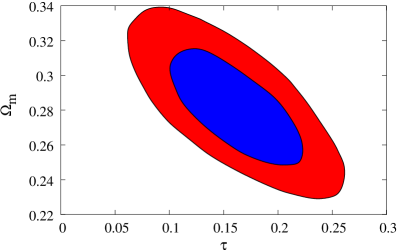
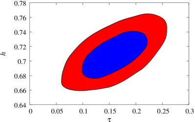
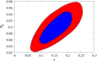
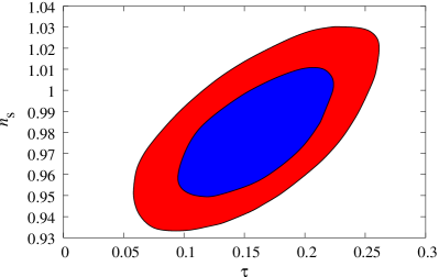
Figure 1: 68% (inner, blue) and 95% (outer, red) contours in the plane of $\tau)$ versus $\Omega_{m}$, $h$, $\sigma_{8}$ and $n_{s}$, respectively, using all measurements.

III.3 Neutrino mass

Both the CMB and LSS are important as tracers of neutrino mass. At the time of decoupling, neutrinos are still relativistic, but become nonrelativistic later in the evolution of the universe if their mass is sufficiently high. Neutrinos free-stream out of their potential wells, erasing their own perturbations on smaller scales. Below this suppression scale the power spectrum shape is the same as in regular CDM models, so on small scales the only consequence is the suppression of the amplitude relative to large scales. In the matter power spectrum neutrinos leave a characteristic feature at the transition scale. The actual shape of the transition depends on the individual masses of neutrinos and not just on their sum. For masses of interest today the transition is occurring around $k=0.1h$/Mpc, which are the scales measured by SDSS-gal. Neutrinos with mass below 2eV are still relativistic when they enter the horizon for scales around $k=0.1h$/Mpc and are either relativistic or quasi-relativistic at the time of recombination, $z\sim 1100$. As a result neutrinos cannot be treated as a nonrelativistic component with regard to the CMB and are not completely degenerate with the other relativistic components in the CMB.

From the joint analysis we find for the sum of all masses (table 3)

$$\sum m_{\nu}<0.42{\rm eV}~{}(0.67{\rm eV})~{}{\rm(3~{}families)},$$ (4)

at 95% (99.9%) c.l. for a single component and assuming no running, as was done in all of the work to date. Our constraints improve upon WMAP+SDSS-gal, where we find $m_{\nu}<1.54$eV and upon WMAP+2dF constraints, where $m_{\nu}<0.69$eV was found by combining WMAP and 2dF with the bias determination from the bispectrum analysis (Verde et al., 2002).

If running and tensors are allowed, the parameter space expands. In this case, we find $m_{\nu}<0.66~{}(0.93){\rm eV}$. Much of this is caused by running: as discussed in Seljak et al. (2004) running and neutrino mass are anti-correlated. Negative runnings as large as -0.04 and neutrino masses as high as 1.5eV are allowed at 2-sigma. Running is poorly motivated by inflationary models and there is no evidence for it in the current data, so adopting the inflationary prior with no running is reasonable, but one should be aware that the limits are model dependent.

The constraint from equation 4 is remarkably tight and implies the upper limit on neutrino mass assuming degeneracy is 0.14eV at 95% c.l. Our constraint has been obtained assuming 3 degenerate mass neutrino families, but if the neutrino mass splittings are small the constraints on the sum are almost the same even if individual masses are not identical. If the masses are very large compared to mass splittings then the neutrino masses are close to degenerate. However, our upper limit is so low that including mass splittings is necessary. Super-Kamionkande (SK) results find neutrino mass squared difference $\delta m_{23}=2.5\times 10^{-3}{\rm eV}^{2}$ Fukuda et al. (1998); Collaboration (2004), while solar neutrino constraints find neutrino mass squared difference $\delta m_{12}=8\times 10^{-5}{\rm eV}^{2}$ Bahcall et al. (2002); Ahmad et al. (2001); Bahcall et al. (2004). This gives one neutrino family with minimum mass around 0.05eV and another with minimum mass close to 0.007eV. Since only the mass difference is measured, it is in principle possible that the actual neutrino masses are larger than that. Our constraints in combination with SK and solar neutrino constraints limit the mass of the neutrino families to

$$m_{1}<0.13{\rm eV},\,\,\,\,\,m_{2}<0.13{\rm eV},\,\,\,\,\,m_{3}<0.14{\rm eV},$$ (5)

all at 95% c.l. These limits essentially exclude the range of masses argued by the Heidelberg-Moscow experiment of neutrinoless double beta decay if neutrinos are Majorana particles Klapdor-Kleingrothaus (2003), although the two results may still be compatible given all the uncertainties in nuclear matrix element calculations. From $\Delta m/m\sim\Delta m^{2}/2m$ with $m\sim 0.13$eV we find the neutrino masses are not degenerate, but the limits are still weak: the ratios must satisfy

$${m_{3}\over m_{1}}>1.1,\,\,\,\,\,1.1<{m_{3}\over m_{2}}<7,$$ (6)

where the upper limit on $m_{3}/m_{2}$ is determined solely from SK and solar neutrino constraints.

The mass limits presented above are based on 3 degenerate massive neutrino families. If one assumes a model with 3 massless families and 1 massive family (such as a sterile neutrino model), as motivated by LSND results Athanassopoulos et al. (1996), then the mass limits on the sum change, since both the CMB and the matter power spectrum change (see figure 6 in Seljak et al. (2004)). These limits are improved as well with the addition of SDSS-lya and SDSS-bias. We find

$$m_{\nu}<0.79{\rm eV}~{}(1.55{\rm eV})~{}{\rm(3+1~{}families)},$$ (7)

at 95 % (99.9%), compared to the WMAP+2dF analysis without bias where the 95% confidence limit is 1.4eV Hannestad (2003) and to the SDSS+WMAP analysis where the limit is 1.37eV Seljak et al. (2004). We have subtracted from the total sum in table 3 the masses of the active neutrinos to obtain the limit in equation 7. These limits are improved by almost a factor of 2 compared to previous analyses. These limits are more model independent, as there is little correlation with running and/or tensors in this model: for the chains with running and tensors we find $m_{\nu}<0.88{\rm eV}~{}(1.40{\rm eV})$ at 95% (99.9%) c.l.

From the LSND experiment the allowed regions are four islands with the lowest mass $m_{\nu}=0.9$eV and the next lowest 1.4eV Maltoni et al. (2003); Athanassopoulos et al. (1996); Hannestad (2003); Pierce and Murayama (2004). Thus the lowest island allowed by LSND results is excluded at 95% c.l. and all the others at 99.9%. Our derived limits will be tested directly with MiniBoone Experiment at Fermilab Stefanski (2002).

III.4 Tensors

Gravity waves (tensors) are predicted in many models of inflation. The simplest single field models of inflation predict a tight relation between tensor amplitude and slope, which we assume here. We choose to parametrize them at the pivot point $k=0.05$/Mpc, just as for the amplitude, slope and running. This pivot differs from that in the WMAP analysis Peiris et al. (2003). While tensors have their largest effect on large scales, within the single field model adopted here the slope is assumed to be determined from the tensor amplitude. Thus there is no need to parametrize tensors on large scales.

For 7-parameter model without running or neutrino mass, the limit on tensors is (table 1)

$${T\over S}<0.36(0.51)$$ (8)

at 95% (99.9%) c.l. This does not change significantly if neutrinos or running are added to the mix (tables 2-3), in the latter case we find $r<0.45(0.64)$. This constraint is nearly a factor of two better than from WMAP analysis, a consequence of tighter constraint on running from the Ly$\alpha$ forest. We return to these constraints below where we discuss inflation.

III.5 Spectral index

Constraints on the scalar spectral index are primarily driven by the WMAP and SDSS-lya combination. Using these two experiments alone one finds $n_{s}=0.990^{+0.032}_{-0.029}$ for the chains with running, compared to $n_{s}=0.962^{+0.054}_{-0.056}$ for WMAP+SDSS-gal+SDSS-bias without SDSS-lya and to $n_{s}=0.975^{+0.028}_{-0.024}$ for the case where all observations are included (table 2). The inclusion of the SDSS Ly$\alpha$ forest thus reduces the error on the primordial slope by a factor of 2. In the absence of running and with bias and SNIa, this constraint improves further to

$$n_{s}=0.981^{+0.019}_{-0.018}\;{}^{+0.040}_{-0.037}\;{}^{+0.061}_{-0.053}.$$ (9)

Note that the scale invariant model $n_{s}=1$ is only 1-sigma away from the best fit. It is remarkable that such a vast range of observational constraints can be reproduced with a scale invariant power spectrum with 4 parameters only, $\Omega_{b}$, $\Omega_{m}$, $h$ and amplitude $\Delta_{\cal R}^{2}$ (plus possibly optical depth $\tau$ to explain the polarization data).

Tensors are positively correlated with the slope (figure 2) and their inclusion increases the best fit slope value to $n_{s}=1.00^{+0.034}_{-0.028}$. All of these are consistent with a scale invariant spectrum and are in a good agreement with the WMAPext+2dF constraint $n_{s}=0.97\pm 0.03$ Spergel et al. (2003). While 2dF gives a slightly redder spectrum than SDSS the differences in different values quoted in the literature reflect mostly the differences in the assumed parameter space, as shown here for the example of tensors.

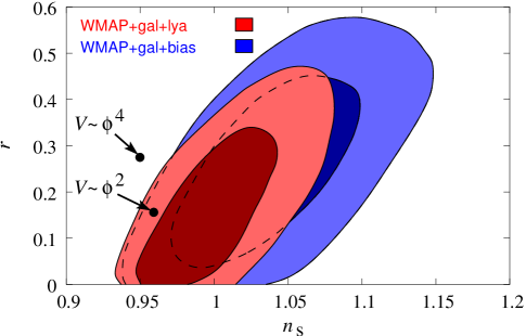
Figure 2: 68% (inner, dark) and 95% (outer, light) contours in the $(r=T/S,n_{s})$ plane with and without SDSS-lya. There is a correlation between tensors and slope $n_{s}$. Inclusion of the Ly$\alpha$ forest significantly reduces the allowed region in this plane. Also shown are the positions of two chaotic inflation models, $V\propto\phi^{2}$ with $N=50$ and $V\propto\phi^{4}$ with $N=60$.

III.6 Running of the spectral index

The issue of the running of the primordial slope has generated a lot of interest lately. WMAP argued for some weak evidence for negative running in their combined analysis, but some of that evidence was based on Lyman alpha constraints by previous workers (Croft et al., 2002; Gnedin and Hamilton, 2002), which were shown to underestimate the errors (Seljak et al., 2003). It was argued that even from WMAP alone, or WMAP+2dF, there is some evidence for running, and the WMAP+SDSS-gal analysis without bias information gave $\alpha_{s}=-0.071\pm 0.044$ (Tegmark et al., 2004b). Similar values have been found from the recent analyses including CBI Readhead et al. (2004) and VSA Rebolo et al. (2004) data. However, much of this effect comes from low $l$ multipoles and a full likelihood analysis of WMAP+SDSS-gal changes this value to $-0.022\pm 0.033$ Slosar et al. (2004). Including the biasing constraints does not really change this result. In the absence of massive neutrinos and tensors we find $\alpha_{s}=-0.022^{+0.030}_{-0.032}$, so $\alpha_{s}=0$ is within one sigma of 0 and the error has not been reduced.

Including SDSS-lya reduces the errors dramatically. The constraint on running from WMAP+SDSS-lya alone is $\alpha_{s}=-0.0026^{+0.013}_{-0.011}$. Including everything this changes slightly to

$$\alpha_{s}=-0.0029^{+0.011}_{-0.010}\;{}^{+0.023}_{-0.018}\;{}^{+0.036}_{-0.026},$$ (10)

which is a factor of 3 improvement over previous constraints. Even with this significant improvement we find no hint of running in the joint analysis. The result is in perfect agreement with no running and 95% of chain elements have $\alpha_{s}>-0.015$. This should be compared to values as low as $\alpha_{s}\sim-0.10$ in figure 3. Similarly low values have been found in recent analyses Readhead et al. (2004); Rebolo et al. (2004). Figure 3 shows old and new constraints in the $(\alpha_{s},n_{s})$ plane, highlighting the dramatic reduction of available parameter space when CMB and Ly$\alpha$ forest data are combined together. The implications of this result for inflation are discussed in the next section.

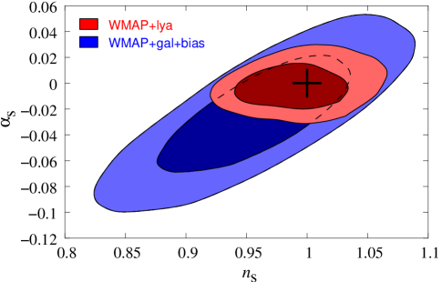
Figure 3: 68% (inner, dark) and 95% (outer, light) contours in the $(\alpha_{s},n_{s})$ plane using WMAP+SDSS-lya versus WMAP+SDSS-gal+bias. Adding the SDSS Ly$\alpha$ forest dramatically reduces the allowed region of parameter space in this plane. Note that the simplest model with $n_{s}=1$ and $\alpha_{s}=0$ is within 68% interval.

If tensors are also included they induce weak anti-correlation with running, so the best fit value becomes $\alpha_{s}=-0.006^{+0.012}_{-0.011}$, which is still perfectly consistent with no running. This is shown in figure 4, where we see that adding SDSS-lya to the mix dramatically reduces the allowed region of parameter space. Specifically, without SDSS-lya, runnings as negative as -0.15 are in the 95% confidence region, a consequence of strong correlation between running and tensors. Our joint analysis eliminates these large negative running solutions. We find no evidence for running in the current data, with or without tensors, despite a factor of 3 reduction in the errors.

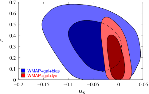
Figure 4: 68% (inner, dark) and 95% (outer, light) contours in the $(\alpha_{s},r)$ plane using WMAP+SDSS-lya versus WMAP+SDSS-gal+bias. Adding the SDSS Ly$\alpha$ forest dramatically reduces the allowed region of parameter space in this plane. Note that the simplest model with $\alpha_{s}=0$ and $r=0$ is within the 68% interval.

Running is correlated with some of the ”nuisance” parameters we marginalize over in the analysis and additional observations constraining these could lead to a further reduction of errors on the primordial slope and its running even with no additional improvements in the observations. For example, in our current treatment of the filtering parameter $k_{F}$ (a generalization of the Jeans length), we assume that the minimum reionization redshift is around 10 with a reheating temperature of 25,000K. If we change the redshift to 7, this leads to an increase in the maximum value of $k_{F}$ allowed. In this case we find for WMAP+SDSS-lya analysis the running changes from $\alpha_{s}=0.0017$ to -0.0045, with an error around 0.01 (see table 2). If we change this redshift to 4, below its theoretically allowed lower limit of 6.5, to allow for any residual resolution issues in numerical simulations, we find $\alpha_{s}=-0.009$ with comparable errors. All the other parameters change much less. While these changes are small and do not qualitatively change our conclusions, they may be important for the future analyses where smaller errors may be obtained. In all these cases the data prefer a high value of $k_{F}$, i.e. a late epoch of reionization. Independent constraints on the tempetarure evolution of IGM would be helpful to constrain this further.

III.7 Matter density and Hubble parameter

The matter density parameter $\Omega_{m}$ has contributions from cold dark matter, baryons, and neutrinos. We assume spatially flat universe, so matter density $\Omega_{m}$ is related to dark energy density $\Omega_{m}=1-\Omega_{\lambda}$. As emphasized in Bridle et al. (2003), the matter density is still allowed to cover a wide range of values from the present data: in 7-parameter models with running WMAP+SDSS-gal gives $\Omega_{m}=0.269^{+0.041}_{-0.033}$. WMAP+SDSS-lya gives a slightly lower value with comparable error, $\Omega_{m}=0.257^{+0.055}_{-0.048}$ in models with running. Combining WMAP, SDSS-gal and SDSS-lya gives $\Omega_{m}=0.299^{+0.037}_{-0.032}$. Including the bias and SNIa and ignoring running brings the value to

$$0.282^{+0.021}_{-0.020}\;{}^{+0.043}_{-0.043}\;{}^{+0.066}_{-0.067}$$ (11)

which is a factor of 2 improvement over previous constraints. The matter density is correlated with $r$ and inclusion of tensors in the parameter space slightly reduces the density parameter. There is a significant improvement in $(\sigma_{8},\Omega_{m})$ plane with the addition of new data (figure 5).

Despite the improvements the matter density remains strongly correlated with the Hubble parameter $h$, as expected from the fact that $\Omega_{m}h^{2}$ is better determined from the CMB than each parameter separately. This is shown in figure 6 for 6-parameter models for the analysis with and without inclusion of SDSS-lya.

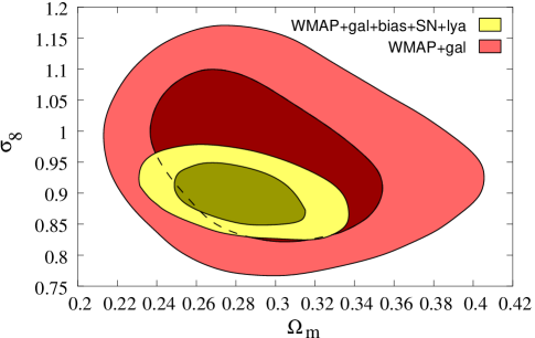
Figure 5: 68% and 95% contours in the $(\Omega_{m},\sigma_{8})$ plane showing previous constraints from WMAP and galaxy clustering with the new data.

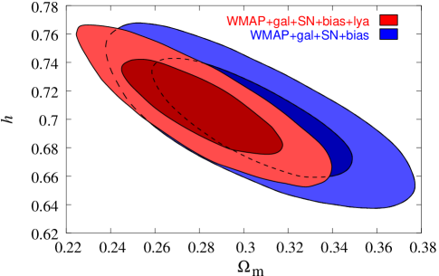
Figure 6: 68% (inner, dark) and 95% (outer, light) contours in the $(\Omega_{m},h)$ plane with and without SDSS-lya. There is a strong correlation between the two parameters because WMAP constrains best the combination $\Omega_{m}h^{2}$.

For the Hubble parameter the best fit value and its error is $h=0.71\pm 0.02$ in 6-parameter space. In 9-parameter space with tensors, massive neutrinos and running we find $h=0.74\pm 0.05$. All of these fits are statistically acceptable and are in good agreement with the HST key project value $h=0.72\pm 0.08$ Freedman et al. (2001), although a different group using almost the same data continues to find a significantly lower value $h=0.58\pm 0.06$ Tammann et al. (2003).

The new data also improve significantly the age of the universe constraint. We find $t_{0}=13.6^{+0.19}_{-0.19}$Gyr, compared to $14.1^{+1.0}_{-0.9}$Gyr found from the WMAP+SDSS-gal analysis Tegmark et al. (2004b).

III.8 Dark energy

So far we have assumed dark energy in the form of a cosmological constant, ${\rm w}=-1$. We now relax this assumption and explore the constraints on w. To maximize the constraints we add to some of the analyses the “gold” SNIa data Riess et al. (2004). Because we do not want to limit ourselves to ${\rm w}>-1$ we assume dark energy does not cluster (${\rm ndyn}=3$ option in CMBFAST4.5). Note that clustering of dark energy vanishes for w=-1 and so if w is close to -1 then it makes very little difference if clustering is included or not. Figure 7 shows the constraints in the $({\rm w},\Omega_{m})$ plane. We find

$${\rm w}=-0.990^{+0.086}_{-0.093}\;{}^{+0.16}_{-0.201}\;{}^{+0.222}_{-0.351}.$$ (12)

We see that ${\rm w}=-1$ is an acceptable solution. This should be compared to ${\rm w}=-1.01^{+0.097}_{-0.12}$ we find in the absence of bias and Ly$\alpha$ forest constraint, to ${\rm w}=-0.91^{+0.13}_{-0.15}$ using the new SNIa data but just some of the LSS constraints Wang and Tegmark (2004), to ${\rm w}=-1.02^{+0.13}_{-0.19}$ using a simple $\Omega_{m}$ prior Riess et al. (2004), and to ${\rm w}=-0.98^{+0.12}_{-0.12}$ from the WMAP 1st year analysis Spergel et al. (2003). It is worth emphasizing the agreement and complementarity of the LSS, CMB, and SNIa constraints: in the absence of SNIa data the constraint is ${\rm w}=-1.02^{+0.15}_{-0.19}$ and w is positively correlated with $\Omega_{m}$ (figure 7). These solutions allow phantom energy models (${\rm w}<-1$) with w as low as -1.5 for low matter density values. On the other hand the two are anticorrelated for the WMAP+SDSS-gal+SNIa data constraints, and phantom energy solutions are allowed for high values of the matter density. Combing the two sets of constraints significantly reduces the parameter space of allowed solutions. All of these different combinations give very consistent results and the median value hardly changes at all and is in all cases very close to ${\rm w}=-1$. Our constraints are a factor of 1.5-2 better than previously published constraints on the dark energy equation of state. Some of the improvement comes from our more sophisticated analysis which includes all of the information previously available and some from the new constraints from the bias and Ly$\alpha$ forest, which further reduce the errors. This is an example of how combining different data sets leads not only to a significant improvement in the accuracy of cosmological parameters, but also how consistency among the different methods gives confidence in the resulting constraints.

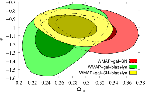
Figure 7: 68% and 95% contours in the $(\Omega_{m},{\rm w})$ plane showing previous constraints without SDSS-lya and bias, constraints without SNIa, and combined constraints. In all cases the data are consistent with a cosmological constant model (${\rm w}=-1$).

The results are weakly model dependent, in the sense that they are sensitive to the parameter space over which one is projecting. If we include tensors and running in the analysis we find

$${\rm w}=-0.908^{+0.077}_{-0.091}\;{}^{+0.143}_{-0.197}\;{}^{+0.192}_{-0.324}~{},$$ (13)

roughly a 1-sigma change in the central value compared to the case without tensors in equation 12. Figure 8 shows that tensors and the equation of state are correlated. The shift in the best fitted value of w reflects a large volume of parameter space associated with $r>0$ models and not any fit improvement when adding tensors and running: $\chi^{2}$ changes only by 1 and there is no need to introduce tensors (or ${\rm w}\neq-1$) to improve the fit to the data. We also find no correlation between the equation of state and running.

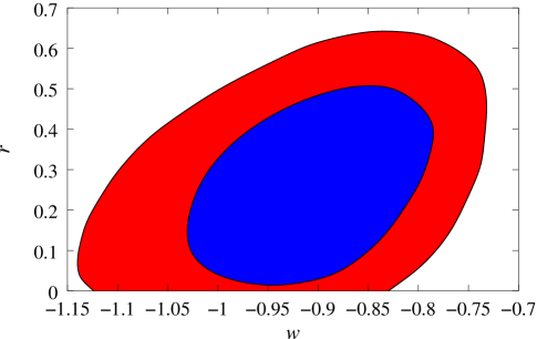
Figure 8: 68% and 95% contours in the $(w,r)$ plane using the WMAP+SDSS-gal+bias+lya+SNIa constraints. The presence of tensors favors a slightly lower value of w, but the quality of the fit is only marginally improved and the cosmological constant model (${\rm w}=-1$) is near the 68% contours.

Our constraints eliminate a significant fraction of previously allowed parameter space, with 95% contours at $-1.19<w<-0.83$ without tensors and at $-1.11<w<-0.77$ with tensors. Thus a large fraction of the parameter space of ”phantom energy” models with ${\rm w}<-1$ Caldwell (2002) and tracker quintessence models with ${\rm w}\sim-0.7$ Steinhardt et al. (1999) appears to be excluded. Other dark energy models which predict ${\rm w}\sim-1$ remain acceptable. It is interesting to note that simplest quintessence solutions with ${\rm w}>-1$ are more acceptable if tensors are present at a level predicted by some inflationary models ($r\sim 0.2$).

We also ran a MCMC simulation exploring a non-constant equation of state. We use a second order expansion

$${\rm w}={\rm w}_{0}+(a-1){\rm w}_{1}+(a-1)^{2}{\rm w}_{2},$$ (14)

where $a=1/(1+z)$ is the expansion factor Linder (2003). The advantage of this expansion is that it is well behaved throughout the history of the universe from early times, when $a\sim 0$, to today ($a=1$). This is in contrast to the often adopted expansion in terms of the redshift, ${\rm w}={\rm w}_{0}+{\rm w}^{\prime}z$, which diverges at high redshift and so can give artificially tight constraints on ${\rm w}^{\prime}$ if CMB (or even BBN) constraints at high redshift are used, without actually saying much about the time dependence of w in the relevant regime $0<z<1$. In contrast, using our expansion $0<z<1$ covers half of the full range of w so ${\rm w}_{1}$ is being constrained in the regime of interest. If we impose ${\rm w}_{2}=0$ then the best fit values and errors we find using all the data are

$${\rm w}_{0} = -0.981^{+0.193}_{-0.193}\;{}^{+0.384}_{-0.373}\;{}^{+0.568}_{-0.521}$$

$${\rm w}_{1} = 0.05^{+0.83}_{-0.65}\;{}^{+1.92}_{-1.13}\;{}^{+2.88}_{-1.38}.$$ (15)

We find that ${\rm w}_{0}=-1$, ${\rm w}_{1}=0$ is well within 1-$\sigma$ contour and very close to the best fit model (figure 9).

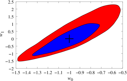
Figure 9: 68% (inner, blue) and 95% (outer, red) contours in the $({\rm w}_{0},{\rm w}_{1})$ plane using WMAP+SDSS-gal+bias+lya+SNIa measurements. We find that the simplest solution, ${\rm w}_{0}=-1$, ${\rm w}_{1}=0$ (marked by a cross), fits the data best.

The parameters ${\rm w}_{0}$, ${\rm w}_{1}$ and ${\rm w}_{2}$ are strongly correlated, as shown in figure 9 for the first two, so the error on ${\rm w}_{0}$ has expanded by a factor of 2 compared to the constant equation of state case. We can explore less model dependent constraints on ${\rm w}(z)$ by computing the median and 1, 2-$\sigma$ intervals from MCMC outputs at any redshift. Over a narrow range of redshift these contours will be nearly model independent as long as the equation of state is a relatively smooth function of redshift. We find that the data constrain best the equation of state w at $z=0.3$, where we find ${\rm w}(z=0.3)=-1.011^{+0.095}_{-0.099}\;{}^{+0.176}_{-0.215}\;{}^{+0.264}_{-0.357}.$ Thus $z=0.3$ is the pivot point for the current measurements of equation of state and the constraint here is nearly model independent. This is confirmed by our analysis with ${\rm w}_{2}$. In this case we find severe degeneracies among the 3 paramaters, but the value at $z=0.3$ is

$${\rm w}(z=0.3)=-0.981^{+0.106}_{-0.120}\;{}^{+0.205}_{-0.249}\;{}^{+0.269}_{-0.386},$$ (16)

which is nearly the same as for the two parameter analysis with ${\rm w}_{2}=0$. These constraints are shown in figure 10.

The corresponding constraint at $z=1$ for two parameter (${\rm w}_{0}$, ${\rm w}_{1}$) analysis is ${\rm w}(z=1)=-1.00^{+0.17}_{-0.28}\;{}^{+0.27}_{-0.66}\;{}^{+0.33}_{-1.00}$. Adding ${\rm w}_{2}$ we find

$${\rm w}(z=1)=-1.03^{+0.21}_{-0.28}\;{}^{+0.39}_{-0.58}\;{}^{+0.52}_{-0.85},$$ (17)

so 1-$\sigma$ contours are nearly the same, while 2 and 3-$\sigma$ contours expand in the positive direction and shrink in the negative direction compared to 2-parameter analysis. This value is thus also relatively independent of parametrization.

Adding tensors and running to the 3-parameter expanasion of w gives,

$${\rm w}(z=0.3)=-0.914^{+0.089}_{-0.106}\;{}^{+0.169}_{-0.225}\;{}^{+0.229}_{-0.343}$$ (18)

and

$${\rm w}(z=1.0)=-0.93^{+0.21}_{-0.25}\;{}^{+0.35}_{-0.56}\;{}^{+0.48}_{-0.90}.$$ (19)

This is shown in figure 11. Thus, in either case, there is no evidence for any time dependence of the equation of state and its value is remarkably close to -1 even at $z=1$. As for a constant w analysis we find that tensors increase the preferred value of w by about 0.1. These constraints on the time dependence of w are significantly better compared to the 0.8-0.9 allowed variation between $z=0$ and $z=1$ found previously Riess et al. (2004). Ly$\alpha$ forest analysis measures the growth of structure in the range $2<z<4$ and so helps in constraining models with a significant component of dark energy present at $z>2$ Mandelbaum et al. (2003).

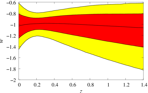
Figure 10: Median (central line), 68% (inner, red) and 95% (outer, yellow) intervals of ${\rm w}(z)$ using all the data in the chains without tensors and with a 3 parameter expansion of equation of state with respect to the expansion factor. Very similar results are found for the 2 parameter expansion of w, so the constraints are reasonably model independent as long as w is a smooth function of redshift. We find that the simplest solution, ${\rm w}=-1$, fits the data at all redshifts.

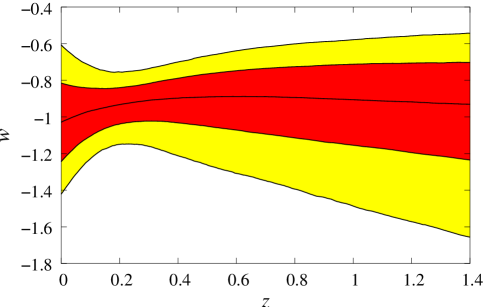
Figure 11: Same as figure 10 but for MCMC with tensors.

IV Implications for inflation

Inflation is currently the leading paradigm for explaining the generation of structure in the universe. Inflation, an epoch of accelerated expansion in the universe, explains why the universe is approximately homogeneous and isotropic and why it is flat Guth (1981); Sato (1981); Albrecht and Steinhardt (1982); Linde (1982). During this accelerated expansion quantum fluctuations are transformed into classical fluctuations when they cross the horizon (i.e., their wavelength exceeds the Hubble length during inflation) and can subsequently be observed as perturbations in the gravitational metric Mukhanov and Chibisov (1981); Guth and Pi (1982); Bardeen et al. (1983); Hawking (1982); Starobinsky (1982). A generic prediction of a single field inflation models is that the perturbations are adiabatic (meaning that all the species in the universe are unperturbed on large scales except for the overall shift caused by the perturbation in the metric) and Gaussian. These predictions, together with flatness ($K=0$), have been explicitly assumed in our analysis.

We note here that cyclic/ekpyrotic models Steinhardt and Turok (2002) are an alternative to inflation, which, despite a very different starting point and without a period of accelerated expansion, lead to almost identical predictions as inflation Khoury et al. (2003). Specifically, these models predict no observable tensor contribution, spectral index $n_{s}$ close to unity, and negligible running Khoury et al. (2001). Very specific forms of cyclic potentials have not been explored in much detail in these models and for this reason we will not discuss them explicitly below, but most of our constraints on the form of the inflationary potential can easily be translated into the corresponding constraints on the form of cyclic model potential.

Here we will explore a class of single field inflation models, in which there is a single field responsible for the dynamics of inflation (even though additional fields may be present or even required to end inflation, as in the case of hybrid inflation Linde (1994)). We will assume the early universe is dominated by a minimally coupled scalar field $\phi$, which we will express in Planck mass units setting $8\pi G=1$. During inflation the energy density is dominated by potential $V$. The Hubble parameter $H^{2}=V/3$ is nearly constant and the equation of state is ${\rm w}=p/\rho\sim-1$. Since $H=d\ln a/dt$ it follows that the expansion factor is exponentially increasing with time, $a=a_{\rm end}e^{H(t-t_{\rm end})}$. One can introduce the number of e-folds before the end of inflation at time $t_{0}$ as

$$N=\ln(a_{\rm end}/a_{0})=\int_{t_{0}}^{t{\rm end}}H(t)dt=\int_{\phi_{0}}^{\phi_{\rm end}}{V\over V^{\prime}}d\phi,$$ (20)

which can be computed for any specific form of the potential. Here we will define it to be the number of e-folds before the end of inflation when the pivot point, $k_{\rm pivot}=0.05/$Mpc, crosses the horizon. Note that the usual definition is with respect to the largest observable scale, $k\sim 10^{-3}$/Mpc, which corresponds to $\Delta N=4$ larger number of efolds. The latter number is expected to be between 50-60 efolds for standard inflation (64 for $V\propto\phi^{4}$), but could be as low as 20 or as high as 100 in special cases Liddle and Leach (2003); Dodelson and Hui (2003). For our pivot point choice we will thus adopt $N=50$ as the standard value (60 for $V\propto\phi^{4}$), but also explore more general constraints on it.

If the kinetic energy density were negligible all the time the universe would keep exponentially expanding and there would be no end to inflation. Typically therefore one must have deviations from the pure ${\rm w}=-1$ case. These deviations lead not only to a finite number of efolds, but also break the scale invariance of the primordial power spectrum. Since we know from current observational constraints that $r<1$ and $n_{s}\sim 1$ we can adopt the slow-roll approximation to relate the form of the potential to the observed quantities $r$, $n_{s}$, $\alpha_{s}$, and $\Delta^{2}_{\cal R}$. The slow-roll parameters are defined as Liddle and Lyth (2000)

$$\epsilon_{V} = {1\over 2}\left({V^{\prime}\over V}\right)^{2}$$

$$\eta_{V} = {V^{\prime\prime}\over V}$$

$$\xi_{V} = {V^{\prime}V^{\prime\prime\prime}\over V^{2}}.$$ (21)

Note that in some early literature the 3rd slow-roll parameter $\xi$ was denoted as $\xi^{2}$ to emphasize the point that it is generically of second order in $\epsilon$ or $\eta$ Kosowsky and Turner (1995). We will not use this notation since $\xi$ can be positive or negative and since it does not have to be of second order in the slow-roll expansion.

The relations between the slow-roll parameters and observables are

$$\Delta^{2}_{\cal R} = {V\over 24\pi^{2}\epsilon_{V}}$$

$$r = 16\epsilon_{V}$$

$$n_{s}-1 = -6\epsilon_{V}+2\eta_{V}$$

$$\alpha_{s} = 16\epsilon_{V}\eta_{V}-24\epsilon_{V}^{2}-2\xi_{V}.$$ (22)

As mentioned in the previous section, we assume $r=-8n_{T}$ and do not consider the running of the tensor spectral index, both of which should be valid for single field inflation in the relevant regime.

Traditionally the inflationary models are divided into separate classes depending on the value of first two slow-roll parameters Dodelson et al. (1997); Lyth and Riotto (1999); Liddle and Lyth (2000). Figure 12 shows the distribution in the $(\epsilon_{V},\eta_{V})$ plane. We see that both positive and negative values of $\eta$ are allowed and that there is a strong correlation between the two from the observational constraints, a consequence of positive correlation between tensors and primordial slope. Figure 13 shows the distribution in the $(\eta_{V},\xi_{V})$ plane. Both parameters are consistent with 0. The basic constraints are $\epsilon<0.03$, $-0.04<\eta<0.12$ and $-0.015-<\xi_{V}<0.035$, so all slow roll parameters are small.

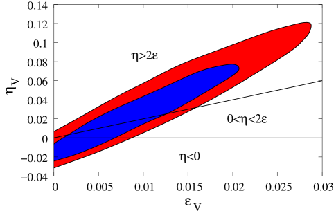
Figure 12: 68% (inner, blue) and 95% (outer, red) contours in the $(\epsilon_{V},\eta_{V})$ plane using all the measurements without running (table 1, 5th column). Also shown are the regions occupied by the 3 classes of inflationary models. All 3 classes of models are allowed, but individual models within each class are constrained. Note that the solutions disfavor low energy models ($\epsilon_{V}=0$) with large positive curvature ($\eta_{V}>0$), typical of hybrid inflation models, as well as models where both $\epsilon_{V}$ is large and $\eta_{V}<\epsilon_{V}/2$, typical of chaotic inflation models with steep potentials.

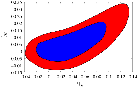
Figure 13: 68% (inner, blue) and 95% (outer, red) contours in the $(\eta_{V},\xi_{V})$ plane from MCMC with running and tensors (table 2, 5th column).

IV.1 Large field models

The simplest inflationary models are the monomial potentials, $V=V_{0}\phi^{p}$, for which the first two parameters are comparable, $\epsilon\sim\eta$, and the curvature is positive, $\eta>0$. These potentials occur in chaotic inflation models Linde (1983). In these models a deviation from scale invariance, $n_{s}-1=-(2+p)/2N$, also implies a significant tensor contribution, $r=4p/N$, while running is negligible, $\alpha_{s}=-2(n_{s}-1)^{2}/(p+2)=-(p+2)/2N^{2}$. Because both slow-roll parameters are of order $(p/\phi)^{2}$ these chaotic inflation-type potentials require a large field, $\phi>1$, to satisfy observationally required $r<1$ and $n_{s}\sim 1$. For this reason these models are sometimes called large field models. While this may limit their particle physics motivation there are brane inspired models where this property can be justified Arkani-Hamed et al. (2003). More generic parametrization of these models in terms of curvature is $0<\eta_{V}<2\epsilon_{V}$.

With the exception of $p=2$, chaotic models are not particularly favored from our analysis. Figure 2 shows the position in the $(r,n_{s})$ plane for two representative cases, $p=2$ and $p=4$. We find that the $V\propto\phi^{2}$ model ($n_{s}=0.96$, $r=0.16$ for N=50) is within the 2-sigma contour, while the $V\propto\phi^{4}$ model ($n_{s}=0.95$, $r=0.27$ for N=60) is outside the 3-sigma contour, since it predicts more tensors and a redder spectrum for that tensor amplitude than observed. Figure 14 shows all chain elements with $n_{s}<1$ converted to $(p,N)$ values using the expressions above. For standard inflation we require $N<60$ and this limits us to $p<3$. Similarly, figure 12 shows that $\epsilon_{V}>\eta_{V}/2$ with large $\epsilon_{V}$ models are disfavored.

For specific models we also minimized $\chi^{2}$ by exploring all of the parameter space of the remaining parameters and compared that to the global minimum in $\chi^{2}$. We find $\Delta\chi^{2}=5$ for the $V\propto\phi^{2}$ model and $\Delta\chi^{2}=13$ for the $V\propto\phi^{4}$ model. These results are in agreement with the MCMC results and show that the latter case is excluded at more than $3-\sigma$ confidence.

Figure 14: Scatter plot of MCMC solutions with $n_{s}<1$ converted into the $(p,N)$ plane assuming relations valid for chaotic inflation models. Here $p$ is the slope of the inflationary potential and $N$ is the number of e-folds. For $N<60$ we require $p<3$.

IV.2 Large positive curvature models

We turn next to models with positive large curvature, $\eta>2\epsilon$. A generic potential of this type can be obtained by adding a constant to the monomial potential, $V=V_{0}(1+c\phi^{p})$, where $c$ is a positive dimensionless constant. These models allow small field solutions to inflation, $\phi\ll 1$, and so are popular for model building in the context of supersymmetry. In this limit, and if dimensionless $c$ is not too large, one has $\epsilon\ll 1$. In such models, inflation never ends (since the potential never drops to zero), so another field must be brought in to accomplish this. Hybrid inflation is an example of such a mechanism Linde (1994). If $\epsilon$ is small then these models predict $r\sim 0$ and $n_{s}>1$ (equations 22, the latter condition requires $\epsilon<\eta/3$). For $p=2$ the slope is constant, $n_{s}-1=2c$ and there is no running, while for $p>2$ running is negative and is given by $\alpha_{s}=-(p-2)/(p-1)[(n_{s}-1)]^{2}/2$. This is always small since a large deviation in the $n_{s}>1$ direction is strongly disfavored, so $\alpha_{s}\sim 0$. Some of these models are disfavored: for $r=0$ and in the absence of running we find $n_{s}<1.0$ at 90% confidence and $n_{s}<1.04$ at 99.9% confidence, so if $\epsilon_{V}\sim 0$ then $\eta_{V}>0.02$ is excluded at 3 sigma. Thus the deviations from scale invariance have to be very small for these models to be acceptable.

IV.3 Large negative curvature models

The most promising models from the observational perspective are negative curvature models, $\eta<0$. As noted above, the main reason that large positive curvature models are disfavored is that in the absence of tensors the data favor $n_{s}<1$, while small positive curvature models are disfavored because they predict large tensors and a red spectrum at the same time, whereas the data are more consistent with blue spectrum if tensors are significant. A generic potential of negative curvature models can be obtained by switching the sign on the hybrid potential form, $V=V_{0}(1-c\phi^{p})$, where $c$ is a positive dimensionless constant. In these models the field $\phi$ is slowly rolling from low to high values until reaching the point where the potential vanishes at $c\phi^{p}=1$, at which point inflation stops. This is a generic scenario of spontaneous symmetry breaking models as in the first working inflation model, that of new inflation Albrecht and Steinhardt (1982). For $p=2$ the slope is again constant at $n_{s}-1=-2c$ and there is no running.

In these models one has $n_{s}-1=-2(p-1)/(p-2)/N$ and $\alpha_{s}=-(p-2)/(p-1)[(n_{s}-1)]^{2}/2$. The running is of order $(n_{s}-1)^{2}/2$ and the prefactor is unity at best, so running is negligible. The slope $n_{s}$ ranges between 0.96 (in the limit of $|p|\rightarrow\infty$,where $n_{s}-1=-2/N$) and 1, in excellent agreement with observational constraints.

One finds good agreement using other potentials proposed in the literature, such as the potential based on one-loop correction in a spontaneous symmetry broken SUSY Dvali et al. (1994). The potential is of the form $V=V_{0}[1+\alpha\ln(\phi/Q)]$. In this model the number of e-folds is of the order $N=\phi^{2}/2\alpha$ (this expression works best if $\alpha\ll 1$). This model predicts $n_{s}-1=-2\alpha[1+3\alpha/2]/\phi^{2}$ and $\alpha_{s}=-(n_{s}-1)^{2}[2\alpha+3\alpha^{2}/2+1/2]/[1+3\alpha/2]^{2}$. Running is again negligible. Solutions with $\phi\ll 1$ require $\alpha\ll\phi^{2}\ll 1$, in which case the slope becomes $n_{s}-1=-1/N=-0.02$ for $N=50$, in excellent agreement with the observed value $n_{s}=0.971^{+0.023}_{-0.019}$.

Many other models in this class also work. A model often mentioned as an example of allowing a large running is the softly broken SUSY model with $V=V_{0}(1-c\phi^{2}(\ln(\phi/\phi_{*})-1/2)/2$. This model has a large 3rd derivative for small field $\phi$, $V^{\prime\prime\prime}/V_{0}=-c/\phi$, so it can lead to large $\xi$ and large runnings. For this model there is an inequality relation between slope and running of the form $\alpha_{s}>-{(n_{s}-1)^{2}\over 4}>-2\times 10^{-3}$, so a large negative running cannot be accommodated in this model for the allowed values of $n_{s}$. Our solutions do not favor large negative runnings anyways, unless one is willing to consider models with massive neutrinos whose mass exceeds 0.3eV, so this model is acceptable, but it can overpredict the running on the positive side.

There are also examples of models which can change from one inflationary case to the other, such as hybrid model with one-loop correction Linde and Riotto (1997), $V=V_{0}\left[1+\alpha\left(\ln(\phi/Q)+{c\over 4}\left({\phi\over\phi_{0}}\right)^{p}\right)\right]$, which under specially arranged conditions causes the slope to change from $n_{s}>1$ on large scale to $n_{s}<1$ on small scale. Again, there is no evidence for such a transition in the data, so there is no need to consider these special cases.

Finally, there are models that predict the simplest possible case of $r=0$, $n_{s}=1$ and $\alpha_{s}=0$ Arkani-Hamed et al. (2004). These models are perfectly acceptable from our data.

While we only surveyed a small subset of inflationary models here, it is clear that their generic prediction is a nearly scale invariant spectrum, $|n_{s}-1|<0.05$, little or no tensors, $r<1$ and small running, $\alpha_{s}\sim 10^{-3}$. All of these predictions agree with our constraints. Running is a particularly powerful test of standard inflationary (and cyclic) models in the sense that if running turned out to be large, a large class of inflationary models would have been eliminated. The original suggestions of running in the WMAP data sparked a lot of theoretical interest in inflationary models with running Kawasaki et al. (2003); Chung et al. (2003), but such models are unnatural in the sense that they require a feature in the potential at exactly the scale of observations today. Our results suggest that the natural prediction of inflation, small running, is confirmed by observations.

V Conclusions

In this paper we performed a joint cosmological analysis of WMAP, the SDSS galaxy power spectrum and its bias, the SDSS Ly$\alpha$ forest power spectrum, and the latest supernovae SNIa sample. We work in the context of current structure formation models, such as inflation or cyclic models, so we assume spatially flat universe and adiabatic initial conditions. We also ignore more exotic components such as warm dark matter. The new ingredients, SDSS Ly$\alpha$ forest and SDSS bias, lead to a significant reduction of the errors on all the parameters. Many parameters are improved in accuracy by factors of two or more. For example, for the amplitude of fluctuations we find $\sigma_{8}=0.90\pm 0.03$ and for the matter density we find $\Omega_{m}=0.28\pm 0.02$, both a significant improvement over previous constraints. From the fundamental physics perspective the highlights of the new constraints are:

1) The scale invariant primordial power spectrum is a remarkably good fit to the data and there is no evidence that the spectral index deviates from the scale invariant value $n_{s}=1$, nor is there any evidence of its running with scale. We also find no evidence of tensors in the joint analysis. The constraints on running have improved by a factor of 3 compared to an analysis without the new Ly$\alpha$ forest constraints. These provide a data point at $2<z<4$ and $k\sim 1$/Mpc, a significantly smaller scale than scales traced by the CMB and galaxies.

2) There is no cosmological evidence of neutrino mass yet. In the standard models with 3 neutrino families we find for the total neutrino mass $\sum m_{\nu}<0.42$eV (95% c.l.). When our analysis is combined with atmospheric and solar neutrino experiments Collaboration (2004); Ahmad et al. (2001) we find that neutrino masses are not degenerate: the most massive neutrino family has to be at least 10% more massive than the least massive family, $m_{3}/m_{1}>1.1$: the mass of the least massive neutrino family has to be $m_{1}<0.13$eV, and that of the most massive neutrino family $m_{3}<0.15$eV, both at 95 % c.l. In alternative models with a 4th massive neutrino family in addition to 3 (nearly) massless ones we find $m_{\nu}<0.79$eV, excluding all of the allowed LSND islands at 95% c.l.

3) Dark energy continues to be best characterized as a standard cosmological constant with constant energy density and equation of state ${\rm w}=-1$. When all the data is combined together the error on w is 0.09, a reduction compared to previously published values Spergel et al. (2003); Wang and Tegmark (2004); Riess et al. (2004). A cosmological constant with ${\rm w}=-1$ is remarkably close to the best fit value for a variety of different subsamples of the data. A significant region of phantom energy parameter space with ${\rm w}<-1$ is excluded, as are some of the tracker quintessence models with ${\rm w}\sim-0.7$. The current data do not support any time dependence of the equation of state.

As the statistical errors are being reduced the required level at which systematics must be controlled increases as well. Our limits on cosmological parameters assume that the errors from the SDSS Ly$\alpha$ forest  SDSS power spectrum shape, SDSS bias, WMAP CMB power spectrum, and the SNIa data are all properly characterized by the authors and that there are no additional sources of systematic error. Each one of these ingredients has to be tested and redundancy is necessary for the results to be believable. In our extensive tests we find no evidence of a disagreement between the different observational inputs, but further tests with these and other data sets are needed to verify and confirm our results. In addition, the upcoming 2 year analysis of WMAP polarization will improve the constraints on the optical depth and reduce the errors on parameters correlated with it.

Tests of the basic model are particularly important for Ly$\alpha$ forest , which is responsible for most of the improvement on the primordial power spectrum shape and amplitude. Despite the extensive tests presented in McDonald et al. (2004c), more work is needed to investigate all possible physical effects that can modify its distribution and to see how these may affect the conclusions reached in this paper. Some of these tests will come from the ongoing work on SDSS data, such as the bispectrum analysis. Similarly, more work is needed to verify the accuracy of simulations with independent hydrodynamic codes. The present analysis, together with its sister papers McDonald et al. (2004b, c), is not the final word on this subject, but merely a first attempt to take advantage of the enormous increase in statistical power given by the SDSS data McDonald et al. (2004a). Current analysis marginalizes over many physical processes that have little or no external constraints and as a result the statistical power of cosmological constraints from the Ly$\alpha$ forest is weakened. Better theoretical understanding of these processes together with external constraints from additional observational tests could lead to a significant reduction of observational errors on the primordial slope and its running even with no additional improvements in the observations.

In summary, adding SDSS Ly$\alpha$ forest and SDSS bias constraints to cosmological parameter estimation leads to a significant improvement in the precision with which the cosmological parameters can be determined. Despite these improvements we find no surprises. Many of these results are not unexpected, but the tightness of the constraints is rapidly eliminating many of the alternative models of structure formation, neutrinos and dark energy. Future cosmological observations and improvements in theoretical modelling will allow us to verify the constraints found here and improve them further. As the constraints become tighter there may be additional surprises awaiting us in the future.

We thank the WMAP and SNIa teams for creating the data sets used in present analysis. Our MCMC simulations were run on a Beowulf cluster at Princeton University, supported in part by NSF grant AST-0216105. US is supported by a fellowship from the David and Lucile Packard Foundation, NASA grants NAG5-1993, NASA NAG5-11489 and NSF grant CAREER-0132953.

Funding for the creation and distribution of the SDSS Archive has been provided by the Alfred P. Sloan Foundation, the Participating Institutions, the National Aeronautics and Space Administration, the National Science Foundation, the U.S. Department of Energy, the Japanese Monbukagakusho, and the Max Planck Society. The SDSS Web site is http://www.sdss.org/.

The SDSS is managed by the Astrophysical Research Consortium (ARC) for the Participating Institutions. The Participating Institutions are The University of Chicago, Fermilab, the Institute for Advanced Study, the Japan Participation Group, The Johns Hopkins University, Los Alamos National Laboratory, the Max-Planck-Institute for Astronomy (MPIA), the Max-Planck-Institute for Astrophysics (MPA), New Mexico State University, University of Pittsburgh, Princeton University, the United States Naval Observatory, and the University of Washington.

References

- Bennett et al. (2003) C. L. Bennett, M. Halpern, G. Hinshaw, N. Jarosik, A. Kogut, M. Limon, S. S. Meyer, L. Page, D. N. Spergel, G. S. Tucker, et al., ApJS 148, 1 (2003).
- Hinshaw et al. (2003) G. Hinshaw, D. N. Spergel, L. Verde, R. S. Hill, S. S. Meyer, C. Barnes, C. L. Bennett, M. Halpern, N. Jarosik, A. Kogut, et al., ApJS 148, 135 (2003).
- Kogut et al. (2003) A. Kogut, D. N. Spergel, C. Barnes, C. L. Bennett, M. Halpern, G. Hinshaw, N. Jarosik, M. Limon, S. S. Meyer, L. Page, et al., ApJS 148, 161 (2003).
- Tegmark et al. (2004a) M. Tegmark, M. R. Blanton, M. A. Strauss, F. Hoyle, D. Schlegel, R. Scoccimarro, M. S. Vogeley, D. H. Weinberg, I. Zehavi, A. Berlind, et al., ApJ 606, 702 (2004a).
- Percival et al. (2001) W. J. Percival, C. M. Baugh, J. Bland-Hawthorn, T. Bridges, R. Cannon, S. Cole, M. Colless, C. Collins, W. Couch, G. Dalton, et al., MNRAS 327, 1297 (2001).
- Pope et al. (2004) A. C. Pope, T. Matsubara, A. S. Szalay, M. R. Blanton, D. J. Eisenstein, J. Gray, B. Jain, N. A. Bahcall, J. Brinkmann, T. Budavari, et al., ApJ 607, 655 (2004).
- Riess et al. (2004) A. G. Riess, L. Strolger, J. Tonry, S. Casertano, H. C. Ferguson, B. Mobasher, P. Challis, A. V. Filippenko, S. Jha, W. Li, et al., ApJ 607, 665 (2004).
- Knop et al. (2003) R. A. Knop, G. Aldering, R. Amanullah, P. Astier, G. Blanc, M. S. Burns, A. Conley, S. E. Deustua, M. Doi, R. Ellis, et al., ApJ 598, 102 (2003).
- Liddle and Lyth (2000) A. R. Liddle and D. H. Lyth, eds., Cosmological inflation and large-scale structure (2000).
- Peiris et al. (2003) H. V. Peiris, E. Komatsu, L. Verde, D. N. Spergel, C. L. Bennett, M. Halpern, G. Hinshaw, N. Jarosik, A. Kogut, M. Limon, et al., ApJS 148, 213 (2003).
- Tegmark et al. (2004b) M. Tegmark, M. A. Strauss, M. R. Blanton, K. Abazajian, S. Dodelson, H. Sandvik, X. Wang, D. H. Weinberg, I. Zehavi, N. A. Bahcall, et al., Phys. Rev. D 69, 103501 (2004b).
- Khoury et al. (2003) J. Khoury, P. J. Steinhardt, and N. Turok, Physical Review Letters 91, 161301 (2003).
- Khoury et al. (2001) J. Khoury, B. A. Ovrut, P. J. Steinhardt, and N. Turok, Phys. Rev. D 64, 123522 (2001).
- Croft et al. (1998) R. A. C. Croft, D. H. Weinberg, N. Katz, and L. Hernquist, ApJ 495, 44 (1998).
- McDonald et al. (2004a) P. McDonald, U. Seljak, S. Burles, D. J. Schlegel, D. H. Weinberg, D. Shih, J. Schaye, D. P. Schneider, J. Brinkmann, R. J. Brunner, et al., ArXiv Astrophysics e-prints (2004a), astro-ph/0405013, eprint astro-ph/0405013.
- York et al. (2000) D. G. York, J. Adelman, J. E. Anderson, S. F. Anderson, J. Annis, N. A. Bahcall, J. A. Bakken, R. Barkhouser, S. Bastian, E. Berman, et al., AJ 120, 1579 (2000).
- Gunn et al. (1998) J. E. Gunn, M. Carr, C. Rockosi, M. Sekiguchi, K. Berry, B. Elms, E. de Haas, Ž. Ivezić, G. Knapp, R. Lupton, et al., AJ 116, 3040 (1998).
- Abazajian et al. (2004) K. Abazajian, J. K. Adelman-McCarthy, M. A. Agüeros, S. S. Allam, K. S. J. Anderson, S. F. Anderson, J. Annis, N. A. Bahcall, I. K. Baldry, S. Bastian, et al. (2004), eprint astro-ph/0403325.
- Croft et al. (2002) R. A. C. Croft, D. H. Weinberg, M. Bolte, S. Burles, L. Hernquist, N. Katz, D. Kirkman, and D. Tytler, ApJ 581, 20 (2002).
- McDonald et al. (2000) P. McDonald, J. Miralda-Escudé, M. Rauch, W. L. W. Sargent, T. A. Barlow, R. Cen, and J. P. Ostriker, ApJ 543, 1 (2000).
- Kim et al. (2003) T. . Kim, M. Viel, M. G. Haehnelt, R. F. Carswell, and S. Cristiani (2003), eprint astro-ph/0308103.
- McDonald et al. (2004b) P. McDonald, U. Seljak, R. Cen, and the SDSS Collaboration, , in preparation (2004b).
- McDonald et al. (2004c) P. McDonald, U. Seljak, R. Cen, and P. Bode, , in preparation (2004c).
- Fukuda et al. (1998) Y. Fukuda, T. Hayakawa, E. Ichihara, K. Inoue, K. Ishihara, H. Ishino, Y. Itow, T. Kajita, J. Kameda, S. Kasuga, et al., Physical Review Letters 81, 1158 (1998).
- Ahmad et al. (2001) Q. R. Ahmad, R. C. Allen, T. C. Andersen, J. D. Anglin, G. Bühler, J. C. Barton, E. W. Beier, M. Bercovitch, J. Bigu, S. Biller, et al., Physical Review Letters 87, 071301 (2001).
- Collaboration (2004) T. S.-K. Collaboration, ArXiv High energy experiment e-prints (2004), eprint hep-ph/0404034.
- Hu et al. (1998) W. Hu, D. J. Eisenstein, and M. Tegmark, Physical Review Letters 80, 5255 (1998).
- Athanassopoulos et al. (1996) C. Athanassopoulos, L. B. Auerbach, R. L. Burman, I. Cohen, D. O. Caldwell, B. D. Dieterle, J. B. Donahue, A. M. Eisner, A. Fazely, F. J. Federspiel, et al., Physical Review Letters 77, 3082 (1996).
- Hannestad (2003) S. Hannestad, Journal of Cosmology and Astro-Particle Physics 5, 4 (2003).
- Pierce and Murayama (2004) A. Pierce and H. Murayama, Physics Letters B 581, 218 (2004).
- Seljak et al. (2004) U. Seljak, A. Makarov, R. Mandelbaum, C. Hirata, N. Padmanabhan, P. McDonald, M. Blanton, M. Tegmark, N. Bahcall, and J. Brinkmann, ArXiv Astrophysics e-prints (2004), eprint astro-ph/0406594.
- Hatton and Cole (1999) S. Hatton and S. Cole, MNRAS 310, 1137 (1999).
- Verde et al. (2002) L. Verde, A. F. Heavens, W. J. Percival, S. Matarrese, C. M. Baugh, J. Bland-Hawthorn, T. Bridges, R. Cannon, S. Cole, M. Colless, et al., MNRAS 335, 432 (2002).
- Hoekstra et al. (2002) H. Hoekstra, L. van Waerbeke, M. D. Gladders, Y. Mellier, and H. K. C. Yee, ApJ 577, 604 (2002).
- Sheldon et al. (2003) E. S. Sheldon, D. E. Johnston, J. A. Frieman, R. Scranton, T. A. McKay, A. J. Connolly, T. Budavari, I. Zehavi, N. Bahcall, J. Brinkmann, et al. (2003).
- Liddle (2004) A. R. Liddle, ArXiv Astrophysics e-prints (2004), eprint astro-ph/0401198.
- Readhead et al. (2004) A. C. S. Readhead, B. S. Mason, C. R. Contaldi, T. J. Pearson, J. R. Bond, S. T. Myers, S. Padin, J. L. Sievers, J. K. Cartwright, M. C. Shepherd, et al., ArXiv e-print astro-ph/0402359 (2004), eprint astro-ph/0402359.
- Rebolo et al. (2004) R. Rebolo, R. A. Battye, P. Carreira, K. Cleary, R. D. Davies, R. J. Davis, C. Dickinson, R. Genova-Santos, K. Grainge, C. M. Gutirrez, et al., ArXiv e-print astro-ph/0402466 (2004), eprint astro-ph/0402466.
- Kuo et al. (2002) C. L. Kuo, P. A. R. Ade, J. J. Bock, C. Cantalupo, M. D. Daub, J. Goldstein, W. L. Holzapfel, A. E. Lange, M. Lueker, M. Newcomb, et al. (2002), eprint arXiv:astro-ph/0212289.
- Spergel et al. (2003) D. N. Spergel, L. Verde, H. V. Peiris, E. Komatsu, M. R. Nolta, C. L. Bennett, M. Halpern, G. Hinshaw, N. Jarosik, A. Kogut, et al., ApJS 148, 175 (2003).
- McDonald et al. (2001) P. McDonald, J. Miralda-Escudé, M. Rauch, W. L. W. Sargent, T. A. Barlow, and R. Cen, ApJ 562, 52 (2001).
- Seljak et al. (2003) U. Seljak, P. McDonald, and A. Makarov, MNRAS 342, L79 (2003).
- Seljak and Zaldarriaga (1996) U. Seljak and M. Zaldarriaga, ApJ 469, 437 (1996).
- Gelman and Rubin (1992) A. Gelman and D. Rubin (1992).
- Verde et al. (2003) L. Verde, H. V. Peiris, D. N. Spergel, M. R. Nolta, C. L. Bennett, M. Halpern, G. Hinshaw, N. Jarosik, A. Kogut, M. Limon, et al., ApJS 148, 195 (2003).
- Slosar et al. (2004) A. Slosar, U. Seljak, and A. Makarov, ArXiv Astrophysics e-prints (2004), eprint astro-ph/0403073.
- Smith et al. (2003) R. E. Smith, J. A. Peacock, A. Jenkins, S. D. M. White, C. S. Frenk, F. R. Pearce, P. A. Thomas, G. Efstathiou, and H. M. P. Couchman, MNRAS 341, 1311 (2003).
- Jing (1998) Y. P. Jing, ApJ 503, L9+ (1998).
- Sheth and Tormen (1999) R. K. Sheth and G. Tormen, MNRAS 308, 119 (1999).
- Seljak and Warren (2004) U. Seljak and M. S. Warren, ArXiv e-print astro-ph/0403698 (2004), eprint astro-ph/0403698.
- Gnedin and Hui (1998) N. Y. Gnedin and L. Hui, MNRAS 296, 44 (1998).
- Cen et al. (1994) R. Cen, J. Miralda-Escude, J. P. Ostriker, and M. Rauch, ApJ 437, L9 (1994).
- Cen et al. (2002) R. Cen, J. P. Ostriker, J. X. Prochaska, and A. M. Wolfe (2002), apJ, submitted (astro-ph/0203524).
- Adelberger et al. (2003) K. L. Adelberger, C. C. Steidel, A. E. Shapley, and M. Pettini, ApJ 584, 45 (2003).
- Schirber et al. (2003) M. Schirber, J. Miralda-Escude, and P. McDonald (2003), apJ, submitted, eprint astro-ph/0307563.
- Croft (2003) R. A. C. Croft, ArXiv Astrophysics e-prints (2003), astro-ph/0310890, eprint astro-ph/0310890.
- Mandelbaum et al. (2003) R. Mandelbaum, P. McDonald, U. Seljak, and R. Cen, MNRAS 344, 776 (2003).
- Zaldarriaga (1997) M. Zaldarriaga, Phys. Rev. D 55, 1822 (1997).
- Bahcall et al. (2002) J. N. Bahcall, M. C. Gonzalez-Garcia, and C. Peña-Garay, Phys. Rev. C 66, 035802 (2002).
- Bahcall et al. (2004) J. N. Bahcall, M. C. Gonzalez-Garcia, and C. Pena-Garay, ArXiv High energy phenomenology e-prints (2004), eprint hep-ph/0406294.
- Klapdor-Kleingrothaus (2003) H. V. Klapdor-Kleingrothaus, in Identification of Dark Matter (2003), pp. 577–+.
- Maltoni et al. (2003) M. Maltoni, T. Schwetz, M. A. Tórtola, and J. W. F. Valle, Nuclear Physics B Proceedings Supplements 114, 203 (2003).
- Stefanski (2002) R. Stefanski, Nuclear Physics B Proceedings Supplements 110, 420 (2002).
- Gnedin and Hamilton (2002) N. Y. Gnedin and A. J. S. Hamilton, MNRAS 334, 107 (2002).
- Bridle et al. (2003) S. L. Bridle, O. Lahav, J. P. Ostriker, and P. J. Steinhardt, Science 299, 1532 (2003).
- Freedman et al. (2001) W. L. Freedman, B. F. Madore, B. K. Gibson, L. Ferrarese, D. D. Kelson, S. Sakai, J. R. Mould, R. C. Kennicutt, H. C. Ford, J. A. Graham, et al., ApJ 553, 47 (2001).
- Tammann et al. (2003) G. A. Tammann, A. Sandage, and A. Saha, in A decade of Hubble Space Telescope science. (2003), pp. 222–+.
- Wang and Tegmark (2004) Y. Wang and M. Tegmark, ArXiv Astrophysics e-prints (2004), eprint astro-ph/0403292.
- Caldwell (2002) R. R. Caldwell, Physics Letters B 545, 23 (2002).
- Steinhardt et al. (1999) P. J. Steinhardt, L. Wang, and I. Zlatev, Phys. Rev. D 59, 123504 (1999).
- Linder (2003) E. V. Linder, Physical Review Letters 90, 091301 (2003).
- Guth (1981) A. H. Guth, Phys. Rev. D 23, 347 (1981).
- Sato (1981) K. Sato, MNRAS 195, 467 (1981).
- Albrecht and Steinhardt (1982) A. Albrecht and P. J. Steinhardt, Physical Review Letters 48, 1220 (1982).
- Linde (1982) A. Linde, Physics Letters B 108, 389 (1982).
- Mukhanov and Chibisov (1981) V. F. Mukhanov and G. V. Chibisov, Journal of Experimental and Theoretical Physics Letteres 33, 532 (1981).
- Guth and Pi (1982) A. H. Guth and S.-Y. Pi, Physical Review Letters 49, 1110 (1982).
- Bardeen et al. (1983) J. M. Bardeen, P. J. Steinhardt, and M. S. Turner, Phys. Rev. D 28, 679 (1983).
- Hawking (1982) S. W. Hawking, Physics Letters B 115, 295 (1982).
- Starobinsky (1982) A. A. Starobinsky, Physics Letters B 117, 175 (1982).
- Steinhardt and Turok (2002) P. J. Steinhardt and N. Turok, Science 296, 1436 (2002).
- Linde (1994) A. Linde, Phys. Rev. D 49, 748 (1994).
- Liddle and Leach (2003) A. R. Liddle and S. M. Leach, Phys. Rev. D 68, 103503 (2003).
- Dodelson and Hui (2003) S. Dodelson and L. Hui, Physical Review Letters 91, 131301 (2003).
- Kosowsky and Turner (1995) A. Kosowsky and M. S. Turner, Phys. Rev. D 52, 1739 (1995).
- Dodelson et al. (1997) S. Dodelson, W. H. Kinney, and E. W. Kolb, Phys. Rev. D 56, 3207 (1997).
- Lyth and Riotto (1999) D. H. Lyth and A. A. Riotto, Phys. Rep. 314, 1 (1999).
- Linde (1983) A. D. Linde, Journal of Experimental and Theoretical Physics Letteres 38, 176 (1983).
- Arkani-Hamed et al. (2003) N. Arkani-Hamed, H. Cheng, P. Creminelli, and L. Randall, Physical Review Letters 90, 221302 (2003).
- Dvali et al. (1994) G. Dvali, Q. Shafi, and R. Schaefer, Physical Review Letters 73, 1886 (1994).
- Linde and Riotto (1997) A. Linde and A. Riotto, Phys. Rev. D 56, 1841 (1997).
- Arkani-Hamed et al. (2004) N. Arkani-Hamed, P. Creminelli, S. Mukohyama, and M. Zaldarriaga, Journal of Cosmology and Astro-Particle Physics 4, 1 (2004).
- Kawasaki et al. (2003) M. Kawasaki, M. Yamaguchi, and J. Yokoyama, Phys. Rev. D 68, 023508 (2003).
- Chung et al. (2003) D. J. Chung, G. Shiu, and M. Trodden, Phys. Rev. D 68, 063501 (2003).