The vertical structure of T Tauri accretion disks
II. Physical conditions in the disk

We present a self-consistent analytical model for the computation of the physical conditions in a steady quasi-Keplerian accretion disk. The method, based on the thin disk approximation, considers the disk as concentric cylinders in which we treat the vertical transfer as in a plane-parallel medium. The formalism generalizes a work by Hubeny (1990), linking the disk temperature distribution to the local energy dissipation and leads to analytical formulae for the temperature distribution which help to understand the behaviour of the radiation propagated inside the disks. One of the main features of our new model is that it can take into account many heating sources. We apply the method first to two sources: viscous dissipation and stellar irradiation. We show that other heating sources like horizontal transfer or irradiation from the ambiant medium can also be taken into account. Using the analytical formulation in the case of a modified Shakura & Sunyaev radial distribution that allow the accretion rate to be partly self-similar in the inner region, and, for an $\alpha$ and $\beta$ prescription of the viscosity, we obtain two-dimensional maps of the temperature, pressure and density in the close environment of low mass young stars. We use these maps to derive the observational properties of the disks such as spectral energy distributions, high resolution spatial images or visibilities in order to underline their different behaviours under different input models.

1 Introduction

Since the initial models of viscous accretion disks of Shakura & Sunyaev (1973) and Lynden-Bell & Pringle (1974), many efforts have focused on the description of the close environment of T Tauri stars (hereafter TTS). In order to reproduce high angular resolution images that became available soon after 1990, various authors have published models of scattered light in large circumstellar structures (Lazareff, Monin, & Pudritz 1990; Whitney & Hartmann 1992). In the last five years, more precise images of edge-on disks have been obtained by the Hubble Space Telescope (HST) and infrared adaptive optics (Burrows et al. 1996; Stapelfeldt et al. 1998; Monin & Bouvier 2000), allowing us to refine the models and the physical parameters used to describe the disks. Most of the time, when interpreting these images, the authors use ad-hoc power laws to extract the physical conditions in the disks, like surface density or the disk scale height. Indeed, these images show that the large-scale flaring disks have a complex vertical structure that must be taken into account in the interpretation of their flat SED.

Up to now, we have access to only a very few constraints on the very central parts of circumstellar disks, since current instruments do not allow us to directly observe within 10 AU of the central object. However, the physics of the inner part of the disks is not expected to be completely different from that in their outer parts, but our knowledge of these central regions of circumstellar disks is restricted to scarce interferometric data and indirect measurements of the inner phenomena via the spectral energy distribution (hereafter SED), the high energy UV and X-ray emission of disks or the measurement of magnetic fields.

The first models used quasi-Keplerian steady accretion disks, expected to be geometrically thin for reasonable values of the accretion rate. They describe the disk as infinitely flat, predicting that the emergent flux has a spectral energy distribution proportional to the power -4/3 of the wavelength in the infrared. However, Rydgren & Zak (1987) showed that most TTS present flatter spectral energy distributions, i.e. decreasing less steeply or even remaining constant over a large domain in the infrared. This discrepancy led Adams, Shu & Lada (1988) to assume that the radial temperature distribution in T Tauri disks is also flatter than in standard accretion disks: if one assumes that the disk thickness flares then the disk intercepts more light from the star at large distances and leads to a variety of SED slopes.

Modeling of the vertical structure of the disks and the associated radiative transfer has been developed by Bell & Lin (1994) focusing their attention on the vertical structure of disks in FU Orionis systems where they explained a possible origin of outbursts. Chiang & Goldreich (1997, 1999) used a semi-analytical model of the circumstellar structure to explain the SEDs of different types of young stars. Recently, D’Alessio et al. (1998, 1999) numerically resolved a complete set of equations to compute the spatial distribution of the temperature and the density that can be constrained by the observed SEDs and two-dimensional images.

Up to now, the models have included various approximations : (i) the magnetic field is ignored; (ii) the viscosity is assumed to depend only on local conditions and (iii) the viscosity is expressed using a simple ad-hoc law. On the other hand, when authors take into account the magnetic field (Shu et al. 1994; Ferreira & Pelletier 1995; Casse & Ferreira 2000a, b), they assume that these magnetic fields do not affect the overall disk structure. As another example, Terquem et al. (1998) and Terquem (1998) showed that gravitational instabilities in the disks may produce waves dissipating viscous energy far from where they are created. Integrating all these effects in a unique model appears to be a difficult task.

Our goal is to develop a radiative model simple enough that it could later on include as many detailed physical processes of the energy transport in the disks as possible, and / or the interaction between the circumstellar matter and the magnetic field. In this paper, we present a new method to process the radiative transfer in circumstellar disks, following the pioneering work by Hubeny (1990) and an initial application in the case of TTS disks by Malbet & Bertout (1991); Malbet (1992). Our results are not fundamentally different from previous models but thanks to the analytical expression of the vertical temperature distribution that we develop, we are able to identify the actual origin of the temperature rise in the upper part of the disk photosphere (Malbet & Bertout 1991). We propose that this formalism can be the starting point for more elaborate models, including magnetic field or viscous transport. As a first step, our new self-consistent analytical model can be used to constrain the physical environment of young stars using images from HST or ground-based large telescopes, as well as millimeter radio-interferometer maps and forthcoming data from large optical interferometers, and especially the ESO VLTI project (Malbet et al. 2000).

Section 2 presents the analytical model derived from hydrostatic and radiative equilibrium, as first described by Hubeny (1990), and extended here to the illumination by an external source. Section 3 describes the application of this model to the specific case of the circumstellar environment of young stellar objects, especially in the case where the accretion rate is not constant at all radii. To illustrate the model and its application, we present and discuss in Sect. 4 some results in the case where the heating by the central source can be neglected and we focus our attention on the production of observable quantities like SEDs, images, and interferometric data including visibility amplitudes and closure phases.

2 Analytical model

In this section, we detail the analytical model for the calculation of the spatial distribution of quantities like the temperature or the density. We use the notations of Hubeny (1990) as much as possible, even if we present the formalism in a slightly different way. The first 3 subsections (2.1, 2.2 and 2.3) are short reminders of the main equations of the problem. The last one (2.4) is the generalization of this formalism to external sources of radiation.

The principle for computing the vertical structure of T Tauri disks is to consider the disk as a set of concentric cylinders of infinitesimal width. Each cylinder is itself regarded as a plane-parallel atmosphere of mixed dust and gas layers. The basic assumption is that the radial radiative transfer of energy is smaller than the vertical transfer, which is true only in the thin disk approximation (Pringle 1981). However, we can still take into account the horizontal transfer as a perturbation for disks of moderate flaring (see in Sect. 2.4.4). We solve the coupled equations of hydrostatic equilibrium and the radiative transfer in each cylinder in order to compute the temperature and density distributions along the $z$-axis at a given radius $r$. In the following sections, when we focus our attention on the vertical structure of the cylinder of radius $r$, we drop the $r$ coordinate unless otherwise specified. We also use the mass column coordinate $m$ in place of the height coordinate $z$:

$$m(z)=\int_{z}^{\infty}\rho(z)\,\mathrm{d}z,$$ (1)

where $M=m(0)=\Sigma/2$ is half the surface density of the disk at radius $r$.

2.1 Initialization stage from the radial structure

For the initial step, we assume a standard geometrically thin disk with a uniform vertical structure at each radius. To fully solve the radial structure, we need:

• the mass per area unit $\Sigma(r)$

• the energy dissipation per area unit $F(r)$

• the opacity law $\chi(T,\rho)$ of the disk material

• the equation of state of the material, $\rho={\cal S}(P,T)$

• the local vertical acceleration field ${\cal G}_{z}(r,z)$, generally inferred from the gravity

where the temperature, density, scale height, pressure and optical thickness laws, respectively $T_{\rm D}$, $P_{\rm D}$, $\rho_{\rm D}$, $h_{\rm D}$ and $\tau_{\rm D}$, are given by the coupled equations:

$$\begin{split}T_{\rm D}^{4}(r)&=\frac{F(r)/2}{1-{\rm e}^{-\tau_{\rm D}(r)}}\\ P_{\rm D}(r)&=-{\cal G}_{z}\big{(}r,h_{\rm D}(r)\big{)}\,\Sigma(r)\\ \rho_{\rm D}(r)&={\cal S}\big{(}P_{\rm D}(r),T_{\rm D}(r)\big{)}\\ h_{\rm D}(r)&=\Sigma(r)/\rho_{\rm D}(r)\\ \tau_{\rm D}(r)&=\Sigma(r)\,\chi\big{(}T_{\rm D}(r),\rho_{\rm D}(r)\big{)}\\ \end{split}$$ (2)

In the optically thin case, an iterative computation is required. One should notice that the mass, energy dissipation and acceleration field distributions do not need to be independent of the temperature or density laws; in this case $\Sigma(r)$, $F(r)$ and ${\cal G}_{z}(r,z)$ are refined at each iteration.

A first refinement is to replace the uniform distribution $\rho_{\rm D}(r)$ by the isothermal density distribution. The resulting radial structure is then the structure given by the so-called standard model (Shakura & Sunyaev 1973; Lynden-Bell & Pringle 1974).

Another improvement consists of replacing the effective temperature by the temperature of the equatorial layer located at $\tau_{\rm D}/2$. As in a stellar atmosphere, we substitute for the first equation of the set of equations (2) the following equation:

$$T_{\rm D}^{4}(r)=\frac{3/4\,F(r)\,(\tau_{\rm D}(r)+2/3)}{1-{\rm e}^{-\tau_{\rm D}(r)}}$$ (3)

2.2 Hydrostatic equilibrium — Density distribution

For a given vertical temperature law, we compute the density distribution from the pressure given by the hydrostatic equilibrium. As the disk is dominated by gravitation of the central star, the partial derivative of ${\cal G}_{z}$ is a constant in the approximation $z\ll r$, and we use a differentiated hydrostatic equilibrium equation for convenience:

$$\frac{\mathrm{d}^{{2}}\,{P}}{\mathrm{d}{m}^{{2}}}=-\frac{1}{{\cal S}(P,T)}\frac{\partial\,{{\cal G}_{z}}}{\partial{z}}$$ (4)

The second order equation Eq. (4) is solved with two following boundary conditions:

1. in the disk mid-plane: the first derivative of $P$ is zero by symmetry.

2. in the outer boundary: $P$ tends to a constant low value, the pressure in the interstellar medium (hereafter ISM). The choice of this limit has almost no influence on the disk structure.

2.3 Radiative equilibrium — Temperature distribution

To complete the calculations of the distributions of the physical quantities, we have to connect the local temperature with the heating sources, remote or local. This is the goal of the radiative transfer described in this section.

Theoretically speaking, the radiative transfer equations can be applied to any kind of radiation. However, common and well-known approximations make them easier to solve provided the radiation is thermalized or isotropic. For instance we can approximate the flux-weighted mean opacity by the Rosseland opacity if the radiation is thermalized with the medium. The Eddington closure relations apply well for isotropic radiation.

We therefore treat separately radiation emitted (from internal heating sources or from external light absorbed by the disk) which is mainly isotropic and thermalized, and the radiation coming from external sources. The latter can also be split into two terms, the attenuated radiation coming from its external source in a certain known direction, and the radiation that has been scattered one or several times which should be mainly isotropic. In the first part of this section, following Hubeny we neglect the radiation by external sources. Later in Sect. 2.4, we will take into account correctly the influence of external radiations.

2.3.1 Energy dissipation in each layer

We first express the temperature as a function of the local production of energy $u$, such as viscous heating, stellar irradiation, disk backwarming, heating by a UV or X radiation field, or the contribution of the energy horizontal transfer. Following the usual notations (Mihalas 1978), we link $u$ to the source function $S$ and the diffuse radiation intensity $I$:

$$4\pi\int_{0}^{\infty}\chi_{\nu}(m)\left[S_{\nu}(m)-J_{\nu}(m)\right]\,\mathrm{d}\nu=\rho(m)u(m)$$ (5)

$${\rm with}\quad J_{\nu}(m)=\int_{-1}^{1}I_{\nu}(m,\mu)\,\mathrm{d}\mu$$ (6)

The conservation of the radiative energy means that in an atmosphere layer, the radiated energy, i.e. the emission of the layer, minus the radiation coming from the neighbouring layers $J_{\nu}(z)$, is exactly equal to the dissipated energy in the layer:

$$S_{\nu}=\frac{\kappa_{\nu}}{\chi_{\nu}}B_{\nu}+\left(1-\frac{\kappa_{\nu}}{\chi_{\nu}}\right)J_{\nu},$$ (7)

Integrating over frequencies, one derives from Eq. (5):

$$\kappa_{B}B=\kappa_{J}J+\frac{u}{4\pi}$$ (8)

where $\kappa_{B}$ and $\kappa_{J}$ are respectively the Planck absorption mean and the usual absorption mean, defined by:

$$\kappa_{B} =\int_{0}^{\infty}(\kappa_{\nu}/\rho)B_{\nu}\,{\rm d}\nu/B$$ (9)

$$\kappa_{J} =\int_{0}^{\infty}(\kappa_{\nu}/\rho)J_{\nu}\,{\rm d}\nu/J$$ (10)

Since $\pi B=\sigma_{B}T^{4}$, the vertical temperature distribution is, by using Eq. (8):

$$T^{4}=\frac{\pi}{\sigma_{B}}\,\frac{\kappa_{J}}{\kappa_{B}}\left[J+\frac{u}{4\pi\kappa_{J}}\right]$$ (11)

In other words, the temperature in a layer is the sum of two contributions: (i) a term proportional to the radiative intensity $J$ transferred by adjacent layers and (ii) a local dissipation term proportional to $u$.

2.3.2 Radiative transfer of the diffuse intensity

We solve the transfer of the diffuse intensity $I$ to determine $J$. The equation of transfer and its two first moments are:

$$\mu\frac{\partial\,{I_{\nu}}}{\partial{z}}(z,\mu) =\chi_{\nu}(z)\left[S_{\nu}(z)-I_{\nu}(z,\mu)\right]$$ (12)

$$\frac{\mathrm{d}\,{H_{\nu}}}{\mathrm{d}{z}}(z) =\chi_{\nu}(z)\left[S_{\nu}(z)-J_{\nu}(z)\right],$$ (13)

$$\frac{\mathrm{d}\,{K_{\nu}}}{\mathrm{d}{z}}(z) =-\chi_{\nu}(z)H_{\nu}(z)$$ (14)

where $J_{\nu}$, $H_{\nu}$ and $K_{\nu}$ are respectively the zeroth, first and second moments of $I_{\nu}$.

By integrating over frequencies one gets:

$$\frac{\mathrm{d}\,{H}}{\mathrm{d}{m}} =-\frac{u}{4\pi}$$ (15)

$$\frac{\mathrm{d}\,{K}}{\mathrm{d}{m}} =\chi_{H}H$$ (16)

In this equation, the flux-averaged opacity $\chi_{H}$ is defined by:

$$\chi_{H}=\int_{0}^{\infty}(\chi_{\nu}/\rho)H_{\nu}\,\mathrm{d}\nu/H,$$ (17)

When integrating the first moment equation Eq. (15) over $m$, one gets:

$$H(m) =H(0)-UM\theta(m)/4\pi$$ (18)

$${\rm with}\quad UM =\int_{0}^{M}u(\zeta)\,\mathrm{d}\zeta$$ (19)

$${\rm and}\quad\theta(m) =\frac{1}{UM}\;\int_{0}^{m}u(\zeta)\,\mathrm{d}\zeta$$ (20)

where $U$ is the total energy dissipation in the upper atmosphere of the disk per surface unit, and $\theta$ the distribution function of the energy dissipation in this atmosphere.

The symmetry conditions in the equatorial plane for the flux $H(m)$ implies that $H(M)=0$, that is $\theta(M)=1$. We therefore get a relation between $H(0)$ and the energy flux dissipated in all atmospheric layers $U$:

$$H(0)=UM/4\pi$$ (21)

Unlike in a stellar atmosphere, energy is locally produced so that the flux is not constant.

Integrating the second moment equation Eq. (16) over $m$, one derives:

$$K =K(0)+H(0)\,\,\left(\tau_{H}-\Delta\tau_{H}\right)$$ (22)

$$\mathrm{with}\quad\tau_{H}(m) =\int_{0}^{m}\chi_{H}(\zeta)\,\mathrm{d}\zeta$$ (23)

$$\mathrm{and}\quad\Delta\tau_{H}(m) =\int_{0}^{m}\chi_{H}(\zeta)\theta(\zeta)\,\mathrm{d}\zeta$$ (24)

where $\tau_{H}$ and $\Delta\tau_{H}$ are respectively the flux weighted and the “energy dissipation weighted” mean optical depths. In a stellar atmosphere, one has $K=K(0)+H(0)\tau_{H}$. Here, $\Delta\tau_{H}$ represents a correction to the flux-weighted mean optical depth due to the decrease of the flux toward the mid-plane of the disk. In the large depth approximation, we have: ${\rm d\,}T^{4}/{\rm d}\tau_{H}\propto H$. Since in a stellar atmosphere, the flux $H$ is constant, $T^{4}\propto H\tau_{H}$, whereas in a disk $H$ decreases with $\tau_{H}$ until $T^{4}\leq H(0)\tau_{H}$, hence the corrective term $\Delta\tau_{H}$.

We then introduce the Eddington factors,

$$f_{K}=\frac{K}{J}\quad{\rm and}\quad f_{H}=\frac{H(0)}{J(0)}.$$ (25)

In the large depth approximation, met in thick parts of the disk, they are respectively equal to 1/3 and 1/2.

2.3.3 Formal solution

Combining Eq. (11), Eq. (22) and Eq. (25), we get the temperature distribution:

$$T^{4}=\frac{\kappa_{J}T_{\mathrm{eff}}^{4}}{4\kappa_{B}f_{K}}\Bigg{[}\left(\tau_{H}-\Delta\tau_{H}+\frac{f_{K}(0)}{f_{H}}\right)+\frac{f_{K}}{M\kappa_{J}}\,\frac{u}{U}\Bigg{]}$$ (26)

with $\sigma_{B}T_{\mathrm{eff}}^{4}=UM$.

In the case of strict thermal equilibrium, the intensity-weighted and flux-weighted mean opacities $\kappa_{J}$ and $\kappa_{H}$ can be substituted by the Planck and Rosseland mean opacities $\kappa_{B}$ and $\kappa_{\mathrm{R}}$.

Equation (26) means that the vertical distribution of the temperature in a disk is similar to its distribution in a stellar atmosphere:

$$T^{4}(\tau)=\frac{\kappa_{J}(\tau)}{4\kappa_{B}\tau f_{K}(\tau)}T_{\mathrm{eff}}^{4}\left[\tau+\frac{f_{K}(0)}{f_{H}}\right],$$ (27)

with two main differences:

• a local term, proportional to the energy dissipation $u$ is added. In a stellar atmosphere no energy dissipation occurs in the intermediate layers. The factor proportional to the density of energy per unit mass $u$, in Eq. (26) is also inversely proportional to the optical depth of the disk, $\kappa_{J}M$. This factor is therefore dominant in zones where the disk is thin.

• the optical depth $\tau$ becomes $\tau_{H}-\Delta\tau_{H}$. The term $\Delta\tau_{H}$ is positive but cannot exceed $\tau_{H}$ depending where the energy dissipation occurs in the vertical structure. The two extreme situations are when the dissipation function is a Dirac function located either in the central plane of the disk, or at the top of the photosphere. In the first situation, $\Delta\tau_{H}=0$ everywhere, whereas in the second one $\Delta\tau_{H}=\tau_{H}$. Above the layers where most dissipation occurs, the correction $\Delta\tau_{H}$ can be ignored and the disk behaves like a stellar atmosphere: there is no local energy source and all radiation comes from deeper layers. In the central layers, $\theta(m)\approx 1$ and $\tau_{H}(m)-\Delta\tau_{H}(m)$ is constant: most energy dissipation occurs in upper layers, and, in other terms there is almost no radiation coming from deeper layers. Therefore the temperature is more or less constant. In the particular case where the energy is dissipated only in the central plane $\tau_{H}-\Delta\tau_{H}=\tau_{H}$ and the disk photosphere behaves like a stellar atmosphere.

2.3.4 Several sources of energy dissipation

In the case where there are several sources of energy dissipation releasing the energy $u_{k}(m)$ in the layer $m$, the formal solution given in Eq. (26) can be split as the sum of the temperature distributions (see appendix A):

$$T^{4}(m)=\sum_{k}\,T_{k}^{4}(m),\\$$ (28)

with the temperature distribution of source $k$,

$$\begin{split}T_{k}^{4}(m)=\frac{\kappa_{J}(T_{\mathrm{eff}})_{k}^{4}}{4\kappa_{B}f_{K}}\Bigg{[}&\left(\tau_{H}-(\Delta\tau_{H})_{k}+\frac{f_{K}(0)}{f_{H}}\right)\\ &+\frac{f_{K}}{M\kappa_{J}}\,\frac{u_{k}}{U_{k}}\Bigg{]},\\ \end{split}$$ (29)

where the effective temperature of the $k$-th source is defined by:

$$\begin{split}\sigma_{B}(T_{\mathrm{eff}})_{k}^{4}&=\int_{0}^{M}\!u_{k}(\zeta)\,\mathrm{d}\zeta\\ &=U_{k}M.\end{split}$$ (30)

The quantity $(\Delta\tau_{H})_{k}$ is defined by Eq. (24) where the vertical distribution function $\theta(m)$ is replaced by the corresponding $k$-th energy source,

$$\theta_{k}(m)=\frac{1}{U_{k}M}\;\int_{0}^{m}u_{k}(\zeta)\,\mathrm{d}\zeta.$$ (31)

We see that when dealing with several sources of energy dissipation, one can treat them separately from the analytical point of view (see Sect. 2.4). However in the full modelization, the field of radiation which defines $J(m)$, $H(m)$, $f_{K}(m)$ and $f_{H}$ must be computed globaly.

2.4 Influence of external radiative sources

Hubeny (1990) already took into account the effect of the irradiation by the central star (see also Hubeny 1991). However, when addressing the influence of the radiation from external sources, we can use Eqs. (28) and (29) taking into account as an additional source of energy dissipation the reprocessing of the incoming radiation. To compute the reprocessed energy $u_{\mathrm{A}}$ and its influence on $(\Delta\tau_{H})_{\mathrm{A}}$, we need to solve the radiative transfer of the direct and scattered incoming radiation.

The flux coming from a central source is highly directional and cannot be processed as isotropic radiation. For convenience, one may split the radiation field into several components, and consider separate partial transfer equations for the individual components. Some of the radiation components may be considred as a source of additional heating. Only the component containing the thermal emission term, $\kappa_{\nu}B_{\nu}$ can be treated with the formalism developed in the previous section. The mean opacities $\kappa_{J}$, $\kappa_{B}$, $\chi_{H}$, and the mean Eddington factors $f_{K}$ and $f_{H}$ are then defined as appropriate averages over the moments of this particular component of the radiation field.

Here, we process separately (i) the radiation from internal heating sources or from external light absorbed and reprocessed in the disk, a radiation which is mainly isotropic and thermalized, and (ii) the radiation coming from external sources which is not absorbed. In this latter case, we again split the incoming radiation into two terms, one attenuated coming directly from its external source in a given known direction, and one that has been scattered once or several times and that should be mainly isotropic.

We use the following notations:

1. $I_{\nu}$: radiation emitted by the disk itself. (All thermal flux related quantities are written without superscript.)

2. $I_{\nu}^{\mathrm{s}}$: radiation coming from external sources and scattered in the disk

3. $I_{\nu}^{0}$: attenuated radiation coming from external sources

4. $u_{\mathrm{V}}$: the energy dissipated locally (e.g. viscosity process)

5. $u_{\mathrm{A}}$: the energy coming from the incident photons absorbed in the disk and reprocessed

This approach is quite similar to Chandrasekhar’s one (Chandrasekhar 1960) and was used by Malbet & Bertout (1991). It consists of writing the equations of transfer for the total intensity $I_{\nu}$ and then deriving equations involving non-local terms $I_{\nu}^{0}$ and $I_{\nu}^{\mathrm{s}}$. Since the radiative transfer of $I_{\nu}$ and non-local terms are treated separately, the coupling between them can be seen either as a loss of energy for the non-local radiation, or as a gain of energy for $I_{\nu}$. The stellar flux can now be seen as energy dissipation similar to that due to viscosity.

2.4.1 Energy reprocessed by the disk

In the presence of an external source of radiation, the energy dissipation term $u_{\mathrm{A}}$ linked to the reprocessing of the radiation coming from external sources and absorbed in the disk is directly linked to the specific intensity of the incoming radiation by:

$$\begin{split}\rho(m)u_{\mathrm{A}}(m)=4\pi\int_{-1}^{+1}\!\!\!\int_{0}^{+\infty}\!\!\kappa_{\nu}(&I_{\nu}^{0}(m,\mu)\\ &+I_{\nu}^{\mathrm{s}}(m,\mu))\,\mathrm{d}\nu\,\mathrm{d}\mu\end{split}$$ (32)

With $J^{0}$ and $J^{\mathrm{s}}$ the frequency-integrated zeroth order moments of $I_{\nu}^{0}$ and $I_{\nu}^{\mathrm{s}}$,

$$J^{0} =\int_{0}^{+\infty}\!\!J_{\nu}^{0}\,\mathrm{d}\nu\quad\mbox{ with }\quad J_{\nu}^{0} =\int_{-1}^{+1}\!I_{\nu}^{0}(\mu)\,\mathrm{d}\mu,$$ (33)

$$J^{\mathrm{s}} =\int_{0}^{+\infty}\!\!J_{\nu}^{\mathrm{s}}\,\mathrm{d}\nu\quad\mbox{ with }\quad J_{\nu}^{\mathrm{s}} =\int_{-1}^{+1}\!I_{\nu}^{\mathrm{s}}(\mu)\,\mathrm{d}\mu,$$ (34)

and, the intensity weighted opacities,

$$\kappa_{J}^{0} =\int_{0}^{+\infty}\!\!(\kappa_{\nu}/\rho)J_{\nu}^{0}\,\mathrm{d}\nu/J^{0},$$ (35)

$$\kappa_{J}^{\mathrm{s}} =\int_{0}^{+\infty}\!\!(\kappa_{\nu}/\rho)J_{\nu}^{\mathrm{s}}\,\mathrm{d}\nu/J^{\mathrm{s}}.$$ (36)

$u_{\mathrm{A}}$ can be expressed as:

$$u_{\mathrm{A}}=4\pi(\kappa_{J}^{0}J^{0}+\kappa_{J}^{\mathrm{s}}J^{\mathrm{s}}),$$ (37)

The energy absorbed $u_{\mathrm{A}}$ is therefore proportional to the mean incident flux and to the absorption coefficient of the medium.

2.4.2 Radiative transfer of the incoming radiation

We study the transfer of the radiative intensities $I^{0}$ and $I^{\mathrm{s}}$ upon which our knowledge of $u_{\mathrm{A}}$ and $(\Delta\tau_{H})_{\mathrm{A}}$ depends. The equations of transfer for the incoming radiation within the frame of coherent isotropic scattering:

$$\mu\frac{\partial\,{I_{\nu}^{0}}}{\partial{z}}(z,\mu) = -\chi_{\nu}I_{\nu}^{0}(z,\mu),$$ (38)

$$\mu\frac{\partial\,{I_{\nu}^{\mathrm{s}}}}{\partial{z}}(z,\mu) = -\chi_{\nu}I_{\nu}^{\mathrm{s}}(z,\mu)\begin{array}[t]{l}+\sigma_{\nu}J_{\nu}^{\mathrm{s}}(z,\mu)\\ +\sigma_{\nu}J_{\nu}^{0}(z,\mu),\end{array}$$ (41)

where $\sigma_{\nu}J_{\nu}^{0}(z,\mu)$ accounts for the scattering of the incoming radiation and $\sigma_{\nu}J_{\nu}^{\mathrm{s}}(z,\mu)$ for multiple scattering.

We define the direction and frequency averaged opacities,

$$\chi_{J}^{0} =\int_{0}^{+\infty}\!\!(\chi_{\nu}/\rho)J_{\nu}^{0}\,\mathrm{d}\nu/J^{0};$$ (42)

$$\chi_{H}^{0} =\int_{0}^{+\infty}\!\!(\chi_{\nu}/\rho)H_{\nu}^{0}\,\mathrm{d}\nu/H^{0};$$ (43)

$$\sigma_{J}^{0} =\int_{0}^{+\infty}\!\!(\sigma_{\nu}/\rho)J_{\nu}^{0}\,\mathrm{d}\nu/J^{0};$$ (44)

$$\chi_{H}^{\mathrm{s}} =\int_{0}^{+\infty}\!\!(\chi_{\nu}/\rho)H_{\nu}^{\mathrm{s}}\,\mathrm{d}\nu/H^{\mathrm{s}};$$ (45)

where $J_{\nu}^{0}$, $J_{\nu}^{\mathrm{s}}$, and, $H_{\nu}^{0}$, $H_{\nu}^{\mathrm{s}}$ are respectively the zeroth and first moments of $I_{\nu}^{0}$ and $I_{\nu}^{\mathrm{s}}$. Therefore the frequency-integrated zeroth, first and second moments of $I_{\nu}^{0}$ and $I_{\nu}^{\mathrm{s}}$, namely $J^{0}$, $H^{0}$, $K^{0}$ for direct incoming radiation and $J^{\mathrm{s}}$, $H^{\mathrm{s}}$, $K^{\mathrm{s}}$ for scattered incoming radiation, are linked by the following equations:

$$\frac{\mathrm{d}\,{H^{0}}}{\mathrm{d}{m}} =-\chi_{J}^{0}J^{0} \quad\mathrm{and}\quad\frac{\mathrm{d}\,{K^{0}}}{\mathrm{d}{m}} =-\chi_{H}^{0}H^{0}$$ (46)

$$\frac{\mathrm{d}\,{H^{\mathrm{s}}}}{\mathrm{d}{m}} =-\kappa_{J}^{\mathrm{s}}J^{\mathrm{s}}+\sigma_{J}^{0}J^{0} \quad\mathrm{and}\quad\frac{\mathrm{d}\,{K^{\mathrm{s}}}}{\mathrm{d}{m}} =-\chi_{H}^{\mathrm{s}}H^{\mathrm{s}}.$$ (47)

Therefore, the reprocessed energy,

$$u_{\mathrm{A}}(m)=-4\pi\big{(}\frac{\mathrm{d}\,{H^{0}}}{\mathrm{d}{m}}+\frac{\mathrm{d}\,{H^{\mathrm{s}}}}{\mathrm{d}{m}}\big{)},$$ (48)

leads to

$$U_{\mathrm{A}}M =4\pi\big{(}H^{0}(0)+H^{\mathrm{s}}(0)\big{)}$$ (49)

$$\theta_{\mathrm{A}}(m) =1-\frac{H^{0}(m)+H^{\mathrm{s}}(m)}{H^{0}(0)+H^{\mathrm{s}}(0)}$$ (50)

assuming $H^{\mathrm{s}}(M)=0$ and $H^{0}(M)=0$, i.e. assuming that the equatorial plane is a plane of symmetry for the source of external radiation. This is truly the case for a central star or a uniform ambiant medium.

Using the second moment of the incoming and reprocessed radiative equations, we derive $(\Delta\tau_{H})_{\mathrm{A}}$,

$$\begin{split}(\Delta\tau_{H})_{\mathrm{A}}=\tau_{H}+\frac{\omega^{0}\big{[}K^{0}-K^{0}(0)\big{]}+\omega^{\mathrm{s}}\big{[}K^{\mathrm{s}}-K^{\mathrm{s}}(0)\big{]}}{H^{0}(0)+H^{\mathrm{s}}(0)}\end{split}$$ (51)

where we define respectively $\omega^{0}$ and $\omega^{\mathrm{s}}$, the mean ratios of $\chi_{H}$ to $\chi_{H}^{0}$ and $\chi_{H}^{\mathrm{s}}$:

$$\int_{0}^{m}\chi_{H}(\zeta)H^{0}(\zeta)\,\mathrm{d}\zeta =\omega^{0}(m)\int_{0}^{m}\chi_{H}^{0}(\zeta)H^{0}(\zeta)\,\mathrm{d}\zeta$$ (52)

$$\int_{0}^{m}\chi_{H}(\zeta)H^{\mathrm{s}}(\zeta)\,\mathrm{d}\zeta =\omega^{\mathrm{s}}(m)\int_{0}^{m}\chi_{H}^{\mathrm{s}}(\zeta)H^{\mathrm{s}}(\zeta)\,\mathrm{d}\zeta.$$ (53)

If the radiation is absorbed in a geometrically thin layer, where the temperature and density are more or less constant, then $\omega^{0}\approx\chi_{H}/\chi_{H}^{0}$. It is the ratio of the absorption of reprocessed radiation (generally in the thermal infrared) to the absorption of incoming radiation (often in the visible, or UV, or X-ray domain). In the case of a hot source like stellar irradiation or a UV field, this ratio is expected to be less than unity.

Finally the contribution of the incoming radiation source to the temperature distribution is:

$${T_{\mathrm{A}}}^{4}(m) = \frac{\kappa_{J}}{4\kappa_{B}f_{K}}\;(T_{\mathrm{eff}})_{\mathrm{A}}^{4}$$

$$\bigg{[}\frac{\omega^{0}\big{[}K^{0}(0)-K^{0}\big{]}+\omega^{\mathrm{s}}\big{[}K^{\mathrm{s}}(0)-K^{\mathrm{s}}\big{]}}{H^{0}(0)+H^{\mathrm{s}}(0)}$$

$$+\frac{f_{K}(0)}{f_{H}}+\frac{f_{K}}{M\kappa_{J}}\,\frac{\kappa_{J}^{0}J^{0}+\kappa_{J}^{\mathrm{s}}J^{\mathrm{s}}}{H^{0}(0)+H^{\mathrm{s}}(0)}\bigg{]}$$

We show in Appendix B how to compute $J^{0}(m)$, $J^{\mathrm{s}}(m)$, $H^{0}(m)$, and $H^{\mathrm{s}}(m)$ in the case of an external point-like source where the irradiation from the central source is highly collimated. As demonstrated in Sect. 2.3.4, the temperature vertical structure of a sum of point-like sources is the sum of the temperatures computed for each source to the fourth power.

2.4.3 Interpretation

In this section, we discuss in detail the physical interpretation of the complex Eq. (2.4.2). Since we know how to add the contributions of various energy sources by using Eqs. (28) and (29), we can restrict ourselves to a point-like source located at infinity without losing generality. An extended source will then be processed as the sum of point-like sources.

The dependence of the central temperature to the incoming stellar radiation is relatively simple. Since the topmost layer emits half upward to the outside and half downward toward the inner layers, the latter ones receive half of the emission. Their effective temperature is then ${T_{\mathrm{A}}}/2^{1/4}$. Since there is no flux inside (for $\tau\gg 1$), the temperature is constant and equal to this temperature. This intuitive result is compatible with Eq. (2.4.2). As a matter of fact, if $\mu^{0}$ is the cosine angle of the incoming radiation and since $K=\mu^{0}H$, the first term in the square brackets is of the order of $\omega^{0}\mu^{0}$. For a slanted incident stellar radiation, we have $\mu^{0}\ll 1$ and therefore $\omega^{0}\mu^{0}\ll 1$. Deep inside the disk, the third term, evanescent since the incoming radiation is absorbed, is also negligible. The brackets reduce to $f_{K}(0)/f_{H}\approx 2/3$. The central temperature is therefore smaller than the effective temperature ${T_{\mathrm{A}}}$ by a factor $\approx 2^{-1/4}$. In conclusion, half of the absorbed energy is irradiated by the hot topmost layer and another half by the cooler inner layers.

At the surface, the third term in the square brackets reduces to $1/(\mu^{0}\omega^{0})$ by using $J^{0}=H/\mu^{0}$ and is dominant. The temperature is therefore much higher than the effective temperature. This fact is explained in Malbet & Bertout (1991): the topmost layer, vertically optically thin but radially optically thick, absorbs almost all stellar light. This layer is superheated by a factor of $(1/\mu^{0})^{1/4}$. Chiang & Goldreich (1997) refined this view by multiplying the term $1/\mu^{0}$ by $1/\omega^{0}$. The first factor is a pure geometrical effect of the slanted incidence whereas the second one comes from the difference between the opacities for the visible incoming radiation and the infrared reprocessed radiation.

2.4.4 Overview of other heating sources

The flux radiation from the ISM can be processed on the same basis as the stellar irradiation. The main difference is that the ISM does not irradiate in a particular direction. If we assume that it consists of an isotropic black body radiation of characteristic temperature $T_{\rm ISM}$, we can apply Eq. (63) within the two-stream approximation (i.e. with $\mu^{*}=1/\sqrt{3}$ using the definition given in Sect. 3.2.2) and we can demonstrate that the contribution of the ISM radiation is a constant. In fact, if the ISM is the unique source of irradiation, the disk would be isothermal.

All other radiative sources can be treated exactly as the central star. If they are extended, the previous results derived for point-like sources are integrated over angles.

The radial extent of the disk is much larger than the vertical one. We can therefore apply the approximations of large depth to the horizontal transfer. This hypothesis, combined with the LTE approximation, allows us to write the horizontal flux $H_{r}$ as:

$$H_{r}=-\frac{4}{3\pi(\rho\kappa_{\mathrm{R}})}T^{3}\frac{\partial\,{T}}{\partial{r}}$$ (55)

The local energy gain for the material between $r$ and $r+{\rm d}r$ is $4\pi(H_{r}(r+{\rm d}r)-H_{r}(r))$. One then derives the heating per unit of mass of material that allow us to self-consistently compute the correction to the vertical transfer, in the case $H_{r}\ll H$:

$$u_{H}=\frac{4\pi}{\rho}\frac{\partial\,{H_{r}}}{\partial{r}}\quad$$ (56)

3 Application to T Tauri disks

The two main heating sources in the case of T Tauri disks are the viscous dissipation and the stellar light absorption. We apply our general equations in this frame.

3.1 Approximations

All the terms $\tau_{H}$, $\kappa_{H}$, etc., are dependent on the structure. Moreover $f_{K}$ and $f_{H}$, are not known a priori. Therefore we will seek a self-consistent iterative method able to determine these quantities.

We now make two approximations concerning the opacities: the diffuse intensity is a Planck distribution at the local temperature and the radiation coming from a external source is also a Planck distribution at the temperature of the source $T^{*}$. We then derive:

• $\kappa_{J}=\kappa_{B}$, the Planck mean opacity

• $\kappa_{J}^{0}=\kappa_{J}^{\mathrm{s}}=\kappa_{B}^{*}$, the mean opacity for a black body radiation at $T^{*}$ through a medium at temperature $T$.

• $\kappa_{H}=\kappa_{\mathrm{R}}$, the Rosseland mean opacity

Since the scope of this paper is to present analytical solutions and simple numerical applications, we use the gray Rosseland opacities given by Bell & Lin (1994). We also use the gray approximation $\kappa_{B}=\kappa_{B}^{*}=\kappa_{\mathrm{R}}$ and ignore diffusion. Therefore $\omega^{\mathrm{s}}=\omega^{0}$ that we now call $\omega$

The $f_{H}$ and $f_{K}$ values will be close to 1/2 and 1/3. These approximations are only valid at large depths, but we refine these values in optically thin zones at each iteration, as well as for $\omega$.

3.2 Vertical temperature distribution

3.2.1 Viscous heating at each layer in the disk

We consider here an energy density per mass unit which depends on local conditions. The energy dissipation per mass unit due to viscosity is given by Franck, King & Raine (1985):

$$u_{\mathrm{V}}(m)=\nu_{\rm visc}(m)\left(r\frac{\mathrm{d}\,{\Omega}}{\mathrm{d}{r}}\right)^{2}$$ (57)

In the case of a thin Keplerian disk we get:

$$u_{\mathrm{V}}(m)=\frac{9}{4}\Omega^{2}\nu_{\rm visc}(m)$$ (58)

Since $u_{\mathrm{V}}(m)$ depends vertically only on $\nu_{\rm visc}(m)$, the $\theta_{\mathrm{V}}$ function depends only on the vertical structure of the viscosity $\nu_{\rm visc}$ and of its mass-average $\bar{\nu}_{\rm visc}$.

Up to now there has been no exact description of the viscosity induced by the turbulence. In this paper, we have considered two different types of viscosity:

1. The Shakura-Sunyaev prescription stating that the viscosity is proportional to the local sound speed and local height scale:

   $$\nu_{\rm visc}=\alpha c_{s}h\propto T$$ (59)

   The $\theta_{\mathrm{V}}$ function is therefore the distribution function of the temperature. The term $\tau_{H}-(\Delta\tau_{H})_{\mathrm{V}}$, by definition smaller than $\tau_{H}$, can be much smaller if the temperature peaks at the surface of the photosphere.

2. The $\beta$-prescription, derived from laboratory experiments, and applied to accretion disks by Huré et al. (2000), states that

   $$\nu_{\rm visc}=\beta\Omega r^{2}$$ (60)

   where $\beta$ is a constant ranging from $10^{-5}$ to $10^{-3}$. Here the viscosity is uniform along the vertical axis and does not depend on the temperature distribution of the disk.

3.2.2 Heating by the central stellar source

With the approximations of Sect. 3.1, there is no reason to distinguish the two specific intensities $I^{0}$ and $I^{s}$. If we call $I^{*}=I^{0}+I^{s}$, then we find an analytical solution very similar to Eq. (28) of from Malbet & Bertout (1991):

$$T_{\mathrm{A}}^{4} =\displaystyle\frac{\pi\kappa_{J}H^{*}(0)}{f_{K}\kappa_{B}\sigma_{B}}\bigg{[} \omega^{*}\frac{K^{*}(0)-K^{*}}{H^{*}(0)}$$ (61)

$$+\frac{f_{K}(0)}{f_{H}}+\frac{f_{K}\kappa^{*}_{J}J^{*}}{\kappa_{J}H^{*}(0)}\bigg{]}$$

where the quantities linked to the star incoming radiation are superscripted with $*$. The only difference is the presence of $\omega^{*}$ which is not a priori equal to 1 as noted by D’Alessio et al. (1998).

We derive $J^{*}(0)$ and $H^{*}(0)$ from the geometrical properties of the system using the approximation described by Ruden & Pollack (1991). The star is seen by the disk as a point-like source. It is valid beyond a few stellar radii; in the inner parts this is not the case, nevertheless reprocessing is seldom dominant in this region (see Fig. 3 of D’Alessio et al. 1998). A point-like source equivalent to the star must present the same values for $J^{*}(0)$ and $H^{*}(0)$. The incidence angle is given by:

$$\mu^{*}=H^{*}(0)/J^{*}(0)$$ (62)

One finally obtains, using the gray optical depth $\tau$, the same expression (33) of Malbet & Bertout (1991) except for the factor $\omega^{*}$ already discussed in the previous section,

$$T_{\mathrm{A}}^{4} =\displaystyle\frac{(T_{\mathrm{eff}})_{\mathrm{A}}^{4}}{4f_{K}}\bigg{[} \mu^{*}\omega^{*}\;\left(1-{\rm e}^{-\tau/\mu^{*}}\right)$$ (63)

$$+\frac{f_{K}(0)}{f_{H}}+f_{K}\frac{{\rm e}^{-\tau/\mu^{*}}}{\mu^{*}}\bigg{]}$$

where the effective temperature of the stellar reprocessing is:

$$(T_{\mathrm{eff}})_{\mathrm{A}}^{4}=4\pi H^{*}(0)/\sigma_{B}$$ (64)

3.3 Equation of state — hydrostatic equilibrium

The equation of state in the disk is:

$$P =f_{\rm gas}c_{\rm s}^{2}\rho$$ (65)

$${\rm with}\quad c_{\rm s} =\sqrt{\frac{k_{\rm B}T}{{\cal M}m_{\rm H}}}$$ (66)

First of all, radiation pressure is ignored in Eq. (65) as suggested by Shakura & Sunyaev (1973). If the disk is assumed to be homogeneous and mixed by the turbulence, the mass fraction of gas, $f_{\rm gas}$, is a known function of $T$ and $\rho$, and might even be a constant if evaporation is ignored. The dust is only a few percent of the mass of the disk, so we use $f_{\rm gas}=1$ in the present work.

We also assume that the disk dynamics is dominated by the central star, so that it is Keplerian. Then, in the thin approximation, ${\cal G}_{z}$ is a linear function of $z$. Combined with Eq. (65), the hydrostatic equilibrium and the local height scale become:

$$\frac{\mathrm{d}^{{2}}\,{P}}{\mathrm{d}{m}^{{2}}} =-\frac{c_{\rm s}^{2}\Omega^{2}}{P}$$ (67)

$$h =\frac{c_{\rm s}}{\Omega}$$ (68)

$${\rm with}\quad\Omega =\sqrt{\frac{GM*}{r^{3}}}$$ (69)

3.4 Self-similar accretion model

The radial distribution of energy dissipation for the accretion $U_{\mathrm{V}}(r)$ and the surface density $\Sigma(r)$ are essential parameters for the initialisation step of our code. In order to be as general as possible, we use a prescription with a self-similar accretion rate, instead of the model by Shakura & Sunyaev (1973) which assumes a uniform accretion rate over the disk. We assume that some ejection process removes material away from the close environment of the star within a radius $r_{0}$. A more detailed description of this mechanism can be found in Ferreira & Pelletier (1995). The accretion rate is parametrized as:

$${\dot{M}}(r)=\begin{cases}\displaystyle{\dot{M}}_{\infty}\left(\frac{r}{r_{0}}\right)^{\xi}&\mbox{if}\quad r<r_{0}\\[5.0pt] \displaystyle{\dot{M}}_{\infty}&\mbox{if}\quad r\geq r_{0}\end{cases}$$ (70)

where $0\leq\xi\leq 1$ is the ejection index (see Ferreira & Pelletier 1995) and $r_{0}$ the cut-off radius. When $\xi=0$, this model corresponds exactly to the standard accretion model by Shakura & Sunyaev (1973).

The dissipation per area unit $U_{\mathrm{V}}(r)$ and the mass column $\Sigma(r)$ can then be expressed as:

$$U_{\mathrm{V}}(r) =\frac{3{\cal G}M_{*}{\dot{M}}(r)}{8\pi r^{3}}f(r)$$ (71)

$$\Sigma(r) =\frac{{\dot{M}}(r)}{3\pi\nu_{\rm visc}}f(r)$$ (72)

where $f(r)$ is a factor close to unity at large $r$. Using the same method as Shakura & Sunyaev (1973) we obtain:

$$f(r)=\begin{cases}\displaystyle\frac{1}{1+2\xi}\left[1-\left(\frac{r_{*}}{r}\right)^{\xi+\frac{1}{2}}\right]&\mbox{if $r<r_{0}$}\\[10.0pt] \displaystyle 1-\frac{2\xi}{1+2\xi}\sqrt{\frac{r_{0}}{r}}-\frac{1}{1+2\xi}\left(\frac{r_{*}}{r_{0}}\right)^{\xi}\sqrt{\frac{r_{*}}{r}}&\mbox{if $r\geq r_{0}$}\end{cases}$$ (73)

3.5 The numerical code

Our set of equations are coupled and non-linear. They need to be solved numerically, within the framefork presented below.

The grid: we use a logarithmic radial grid. For each radius we chose a non-uniform vertical grid so that the mass column coordinate $m(z)$ is logarithmically sampled.

Initial conditions: from the radial structure described in Sect. 2.1, we compute an isothermal vertical structure.

Iterative method: Knowing the temperature and mass column, the hydrostatic equilibrium is solved for. We deduce the density and pressure distributions. Then the temperature and optical depth are computed again using the development of Sect. 2.3.2. Subsequent quantities are derived, like the kinematic viscosity. The value of $M(r)$ is refined so that it matches Eq. (72) using the average kinematic viscosity. The mass column grid is computed again with the new value of $M(r)$. The latter step is performed as many times as necessary to reach convergence (typically in ten iterations).

The parameters used for the computations are reported in Table 1.

Table 1: Parameters used in the model

$r_{*}$	$=$	$2\,R_{\odot}$	$M_{*}$	$=$	$0.5\,M_{\odot}$
$T_{*}$	$=$	$4000\,{\rm K}$	$T_{\rm ISM}$	$=$	$15\,{\rm K}$
$r_{0}$	$=$	$100\,r_{*}$	$\alpha$	$=$	$0.01$
$r_{\rm min}$	$=$	$2.2\,R_{\odot}$	$A_{\rm V}$	$=$	$1$
$d$	$=$	$450\,\mbox{pc}$

4 Results and discussion

In this paper, we chose to treat mainly the radiative transfer in the disk. Even if we have developed the formalism of the central source heating, we will ignore its contribution in a first step and concentrate only on the viscous dissipation. In a future paper, we will present the case of heating by the central star. Moreover the heating by the central star becomes dominant at radii larger than a few astronomical units as shown in Fig. 3 of D’Alessio et al. (1998) so the results presented here will be correct only for the inner part of the disk and therefore for the visible and infrared thermal domain.

First, we compute the physical conditions in the disk: temperature, density, optical depth. Then we use these physical conditions to compute astronomical observables like SEDs, millimetric images and interferometric complex visibilities and direct images.

4.1 Physical conditions in the disk

4.1.1 Temperature and density

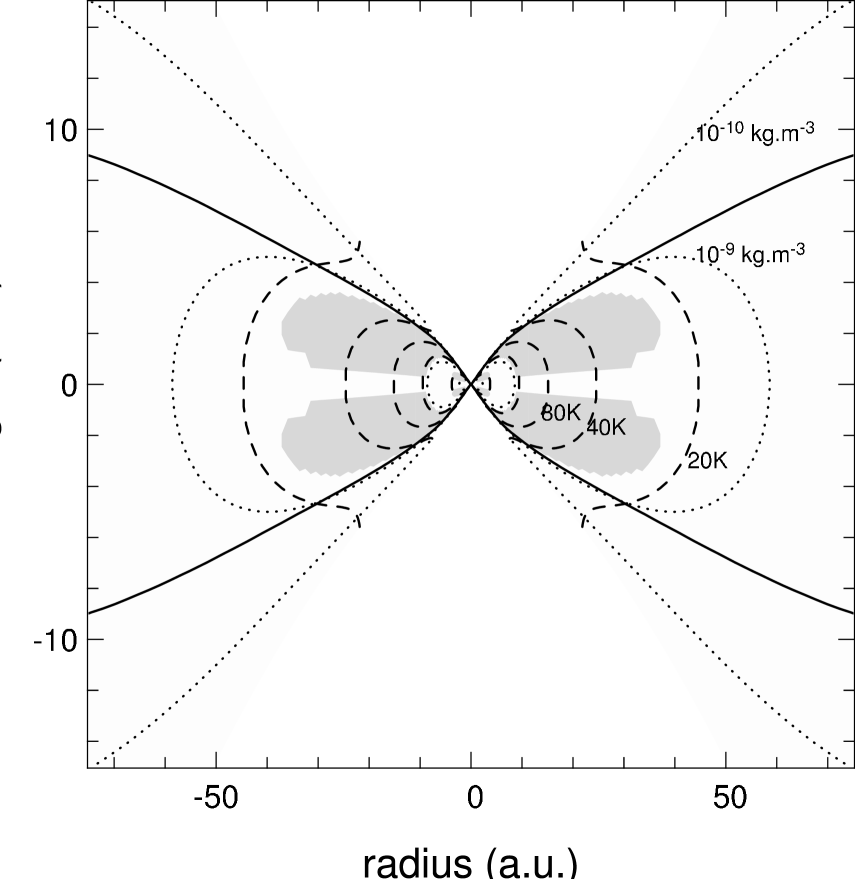
Figure 1: Iso-contour maps of a T Tauri disk with ${\dot{M}}=10^{-5}\,M_{\odot}/\mbox{yr}$. Dashed lines: lines of equal temperature; Dotted lines: lines of equal density; Solid line: limits of the optically thick region ($\tau=1$); Gray zone: zone of instability with respect to the convection.

Figure 2: Radial distribution of the temperature in the central layer and of the effective temperature (located at $\tau=1$).

A map of density and temperature for a standard disk ($\xi=0$) with an accretion rate of $10^{-5}\,M_{\odot}/\mbox{yr}$ is displayed in Fig. 2. The shape of the temperature iso-contours illustrates that the disk temperature is almost constant in the optically thick part, whereas the temperature changes quickly with the altitude in the upper layer. As previously guessed, the disk appears roughly isothermal over the vertical dimension in its inner part.

Figure 2 displays the variation of the temperature with the radius. We verify that the effective temperature, i.e. at $\tau=1$, is proportional to the dissipated flux: it follows an $r^{-3/4}$ law. We stress that the central temperature is much higher than the effective temperature.

We check that the disk is optically thick even at large radii while the geometrical thickness of the disk remains much smaller than unity: if we define the disk surface as the region of optical depth unity, we find $z/r\approx 0.1\mbox{--}0.2$.

The geometry of the density contours displayed in Fig. 2 have a different shape depending whether they are located in the central optically thick part or in the upper optically thin layers. Figure 2 also displays the disk parts which are unstable to convection by computing the Schwarzschild criterion. For the time being, the consequences of this convection are not taken into account in our model.

4.1.2 Column density

Figure 3: Column density in an $\alpha$-disk for two different accretion rates. Solid lines: $\xi=0$; Dashed lines: $\xi=0.5$

Figure 4: Column density in a disk with different viscosity prescriptions. Solid lines: $\alpha=10^{-3},\>10^{-2}$; Dotted lines: $\beta=10^{-4},\>10^{-3}$

Figure 4 shows the mass column density as a function of the radius in the case of a standard $\alpha$-disk with two values of the ejection parameter $\xi$. We take the cut-off $r_{0}$ at 100 stellar radii, i.e. about 1 AU. Two values of the accretion rate have been considered: $10^{-6}$ and $10^{-4}$ $M_{\odot}$/yr. As expected, the radial structure of $\Sigma(r)$ changes in the close environment of the star when $\xi\neq 0$.

Power-laws are often used by observers in the description of the radial structure of disks, though one can see in Fig. 4 that the column density of an $\alpha$-disk cannnot be described with such a law. However, on restricted domains of radius, the mass column in an $\alpha$-disk can be described by the equation

$$\Sigma(r)\approx\Sigma_{i}\,(r/1\,\mbox{AU})^{-q_{i}}\,\mbox{$\mbox{kg.m}^{-2}$}\mbox{ for }r_{i}\leq r\leq r_{i+1}$$ (74)

where the coefficient $q_{i}$ ranges from -0.4 to 1.5 and $\Sigma_{i}$ is a constant. These coefficients are given in Table 2 for two values of the accretion rate.

Table 2: Parameters computed from the model to approximate the surface density by a power law by pieces, sorted by decreasing order of radius domain.

${\dot{M}}=10^{-6}\,M_{\odot}/\mbox{yr}$			${\dot{M}}=10^{-4}\,M_{\odot}/\mbox{yr}$
$\Sigma_{i}$	$q_{i}$	$r_{i}$	$\Sigma_{i}$	$q_{i}$	$r_{i}$
$1\,10^{6}$	$1.5$	40	—	—	—
$4\,10^{3}$	$0.0$	9	$2\,10^{4}$	$0.0$	67
$1.5\,10^{4}$	$0.6$	1	$2.5\,10^{5}$	$0.6$	5
$1.5\,10^{4}$	$1.2$	0.11	$9\,10^{5}$	$1.4$	0.75
$4\,10^{5}$	$-0.3$	0.06	$1.5\,10^{6}$	$-0.5$	0.45

We show in Fig. 4 the influence of $\alpha$ on the structure of the disk. These results are compared with the ones obtained with the $\beta$ viscosity prescription. The general behaviour is somewhat different except for the $1-10\mbox{ AU}$ region. Therefore observing inside 1 AU or outside 10 AU could be decisive in determining the viscosity law.

4.2 Astronomical observables

One of the aims of this work is to compute physical conditions around a young star so that we can calculate the electromagnetic field emerging from this region. This emission can then be analysed by several types of instruments: photometers, spectrographs, imaging cameras, interferometers, etc. The next sections give examples of astronomical observables that can be used to constrain our knowledge of the circumstellar environment.

4.2.1 Spectral energy distribution

Figure 5: Spectral energy distribution ($\lambda F_{\lambda}$ vs. $\lambda$) for different disk models Solid lines: standard disk; Dashed lines: disk with $\xi=0.5$; Dashed & doted lines: standard disk with an inner hole of $8r_{*}$.

Figure 6: Spectral energy distribution ($\lambda F_{\lambda}$ vs. $\lambda$) of the disk model as a function of inclination. Solid lines: pole-on disk. Dashed lines: inclination of $i=45^{o}$. Dotted liness: same inclination without the flaring effect (see text for details).

The spectrophotometry technique gives access to the spectral energy distribution. We integrate along the line of sight the contribution of each disk layer to the emergent flux. In the examples taken for Fig. 6, the SED is significantly altered in the range $1$–$5$ $\mu$m with the self-similar accretion model. The inner hot regions being depleted, the short wavelengths are less present. We assumed an overall extinction of $A_{\rm V}=1$ in the visible and an inner radius of the disk of $r_{\rm min}=1.1$ stellar radius. However, Fig. 6 shows that the SED is significatively different from the one expected from a standard model with a large inner gap.

Figure 6 shows the influence of disk flaring on the intermediate wavelength range of the SED. The difference between the two curves representing the SED of a $45^{o}$-inclined disk lies in the location of the photosphere, i.e. the location of the disk layer that emits most of the emergent flux. In the flaring case, the flux comes from the layer where $\tau=1$, whereas in the so-called no flaring case, the flux comes from the disk equatorial plane but with the same temperature as the effective temperature. This latter case corresponds to the standard radial model where the vertical structure is not taken into account. Even without the reprocessing of the stellar photons, the effect of the vertical extension of the disk atmosphere is therefore not negligible at intermediate wavelengths.

4.2.2 Millimetric images

Figure 7: Emergent millimetric flux from a pole-on disk for several accretion rates and viscosity prescriptions. Upper curves: ${\dot{M}}=10^{-4}\,M_{\odot}/\mbox{yr}$; Lower curves: ${\dot{M}}=10^{-6}\,M_{\odot}/\mbox{yr}$; Solid lines: $\alpha=10^{-2}$; Dashed lines: $\beta=10^{-4}$.

Radio observations can help us discriminate between the two viscosity prescriptions, and especially radio observations in the outer disk, since they are sensitive to the mass column. The disk being optically thin in the millimetric continuum, the flux is given by:

$$F_{\nu}\propto\int_{-\infty}^{+\infty}T(z)\rho(z)\,{\rm d}z\approx\Sigma\bar{T}$$ (75)

Figure 7 compares the millimetric emissivity for an $\alpha$-disk and a $\beta$-disk with the same characteristics. At intermediate radii, the two emissivities are more or less equivalent, however at larger radii the emissivities can follow somewhat different power laws. $F_{\nu}$ is proportionnal to $r^{-3/2}$ for an $\alpha$-disk over the full range, whereas a $\beta$-disk presents a variable power-law exponent. In the domain where the disk is thermalized with the ISM, i.e. at large radii, $F_{\nu}\propto r^{-1/2}$.

4.2.3 Interferometric observables

Figure 8: Visibilities from a disk model as a function of the baseline. Gray: ${\dot{M}}=10^{-4}\,M_{\odot}/\mbox{yr}$; Black: ${\dot{M}}=10^{-6}\,M_{\odot}/\mbox{yr}$. For a given baseline the visibility varies with the position angle; the domain between the minimum and maximum values is filled.

Figure 9: Closure phases as a function of the position angle for a triplet combination of the VLTI auxiliary telescopes. Solid lines: ${\dot{M}}=10^{-4}\,M_{\odot}/\mbox{yr}$. Dotted line: ${\dot{M}}=10^{-6}\,M_{\odot}/\mbox{yr}$ with the largest baseline.

Probing the inner parts of disks requires high angular resolution techniques that can be achieved with present or soon-to-be operated interferometric instruments (Malbet & Bertout 1995). The more massive disks (${\dot{M}}>10^{-6}\,M_{\odot}/\mbox{yr}$) should be resolved by the VLTI and its 100m-baseline, but we should also detect non-zero closure phase.

Figure 9 shows the visibility of a disk as a function of the projected baseline. Since the image is not centro-symmetric, the visibility depends on the position angle. Figure 9 displays the closure phase as a function of the position angle for different telescope combinations in the VLTI for a disk with an important accretion rate (${\dot{M}}=10^{-4}\,M_{\odot}/\mbox{yr}$). As a comparison, the closure phase is displayed for a disk with moderate accretion rate with the widest combination of the VLTI auxiliary telescopes. Because of the natural flaring, a disk that is not seen pole-on does not appear centro-symmetric (as can be noticed in Fig. 10), therefore leading to a non-zero closure phase.

4.2.4 Direct images

Figure 10: Synthetic images of the thermal emission at 2.2 $\mu$m for different inclinations of the disk (from $0^{o}$ to $60^{o}$ by steps of $10^{o}$). ${\dot{M}}=10^{-6}\,M_{\odot}/\mbox{yr}$. The field is 50 mas.

Synthetic infrared images of the disk thermal emission are displayed in Fig. 10 with a field of 50 mas for a distance of $d=450\,\mbox{pc}$. As explained above, they are not centro-symmetric because of the flaring. So far, we have only access to interferometric observations at this scale, so they are only relevant as a step to produce interferometric observables.

5 Conclusion

We have presented a new method to model the vertical structure of accretion disks. This method leads to analytical formulae for the temperature distribution which help to understand the behaviour of the radiation propagated inside the disk. Our model includes two sources of energy dissipation: viscous heating and reprocessing of external radiation like that emitted by the central star. We have applied these analytical results to the case of T Tauri disks in a variety of conditions showing that the method is versatile:

• with a modified Shakura-Sunyaev prescription for a disk with a non-constant accretion rate (Ferreira & Pelletier 1995)

• with a viscosity prescription following either the standard $\alpha$ or the $\beta$ one proposed by Huré et al. (2000)

We are able to simulate the conditions of temperature and density in any part of the circumstellar environment and to compute astronomical observables like SED, optical and millimeter images or interferometric visibilities. This code could be used also as starting conditions in a Monte-Carlo multiple scattering code in order to derive polarization maps.

When completed, this code will offer to observers a tool based on physical parameters to interpret their observations better than ad-hoc models based on power laws often used today.

Appendix A Vertical structure of the temperature with several energy sources

Each source of energy locally contributes to the heating $u_{k}$ (see Sect. 2.3.4). The total local heating is then $u=\sum_{k}u_{k}$ and the energy dissipated per unit of disk surface is then $U=\sum_{k}U_{k}$ with

$$U_{k}M=\int_{0}^{M}\!u_{k}(\zeta)\,\mathrm{d}\zeta.$$ (76)

We now write the vertical distribution of energy dissipation, $\theta$ as a function of the different vertical distributions of the energy source, $\theta_{k}$:

$$\begin{split}\theta(m)&=\int_{0}^{m}u(\zeta)\,\mathrm{d}\zeta/(UM)\\ &=\sum_{k}\frac{U_{k}}{U}\theta_{k}(m)\\ \mbox{with}\quad\theta_{k}(m)&=\int_{0}^{m}u_{k}(\zeta)\,\mathrm{d}\zeta/(U_{k}M)\\ \end{split}$$ (77)

Similarly for $\Delta\tau_{H}$:

$$\begin{split}\Delta\tau_{H}(m)&=\int_{0}^{m}\theta(\zeta)\tau_{H}(\zeta)\,\mathrm{d}\zeta\\ &=\sum_{k}\frac{U_{k}}{U}(\Delta\tau_{H})_{k}\\ \mbox{with}\quad(\Delta\tau_{H})_{k}(m)&=\int_{0}^{m}\theta_{k}(\zeta)\tau_{H}(\zeta)\,\mathrm{d}\zeta\\ \end{split}$$ (78)

Since,

$$\frac{u(m)}{U} =\sum_{k}\frac{U_{k}}{U}\,\,\frac{u_{k}(m)}{U_{k}}$$ (79)

and $\sum_{k}(U_{k}/U)=1$, we can rewrite Eq. (26) by replacing each term in the brackets by a sum over the $k$ sources:

$$\begin{split}T^{4}=\frac{\kappa_{J}T_{\mathrm{eff}}^{4}}{4\kappa_{B}f_{K}}\,\,\sum_{k}\frac{U_{k}}{U}\,\Bigg{[}&\left(\tau_{H}-(\Delta\tau_{H})_{k}+\frac{f_{K}(0)}{f_{H}}\right)\\ &+\frac{f_{K}}{M\kappa_{J}}\,\frac{u_{k}}{U_{k}}\Bigg{]}.\end{split}$$ (80)

If we define the effective temperature of the the $k$-th energy source,

$$\sigma_{B}(T_{\mathrm{eff}})_{k}^{4}=U_{k}M,$$ (81)

then Eq. (26) can be written as the following sum:

$$\begin{split}T^{4}=\sum_{k}\frac{\kappa_{J}(T_{\mathrm{eff}})_{k}^{4}}{4\kappa_{B}f_{K}}\Bigg{[}&\left(\tau_{H}-(\Delta\tau_{H})_{k}+\frac{f_{K}(0)}{f_{H}}\right)\\ &+\frac{f_{K}}{M\kappa_{J}}\,\frac{u_{k}}{U_{k}}\Bigg{]}\end{split}$$ (82)

Therefore the vertical distribution of the temperature for a disk with multiple energy dissipation sources is the same as the sum of the individual temperature distributions using the global radiation in the disk, i.e. with $J$, $H$, $K$, $\tau_{H}$ computed from the global temperature distribution.

Appendix B Incoming radiation field

We show in this appendix how to compute $J^{0}(m)$, $J^{\mathrm{s}}(m)$, $H^{0}(m)$, and $H^{\mathrm{s}}(m)$ in the case of an external point-like source. The intensity of the source is $J^{0}$, giving us a boundary condition to solve the equations of transfer (46) and (47). If we define the optical depths,

$$\tau^{0} =\int_{0}^{m}\chi^{0}_{J}(\zeta)\,\mathrm{d}\zeta$$ (83)

$$\tau^{\mathrm{s}} =\int_{0}^{m}\kappa^{\rm s}_{J}(\zeta)\,\mathrm{d}\zeta$$ (84)

we obtain:

$$J^{0}(m) =J(0){\rm e}^{-\tau^{0}(m)/\mu^{0}}$$ (85)

$$J^{\mathrm{s}}(m) =\Lambda_{\tau^{\mathrm{s}}(m)}\left(\frac{\sigma_{J}^{0}}{\kappa_{J}^{\mathrm{s}}}J^{0}\right)$$ (86)

where $\Lambda$ is a commonly used operator (cf. Mihalas 1978) defined by:

$$\Lambda_{\tau}\left(f\right) =\frac{1}{2}\int_{0}^{+\infty}E_{1}\left|t-\tau\right|f(t)\,\mathrm{d}t$$ (87)

$${\rm and} E_{n}(t) =\int_{1}^{+\infty}u^{-n}{\rm e}^{-ut}\,\mathrm{d}u.$$ (88)

The terms $H^{0}(m)$ and $H^{\mathrm{s}}(m)$ can be computed in the same way as $J^{0}(m)$ and $J^{\mathrm{s}}(m)$:

$$H^{0}(m) =\mu^{0}\,J(0){\rm e}^{-\tau^{0}(m)/\mu^{0}}$$ (89)

$$H^{\mathrm{s}}(m) =\Phi_{\tau^{\mathrm{s}}(m)}\left(\frac{\sigma^{0}_{J}}{\kappa_{J}^{\mathrm{s}}}J^{0}\right)$$ (90)

with

$$\Phi_{\tau}(f) =2\int_{0}^{+\infty}E_{2}|t-\tau|f(t)\,\mathrm{sgn}(t-\tau)\,\mathrm{d}t$$ (91)

where $\mathrm{sgn}(x)$ is the sign function.

References

- Adams, Shu & Lada (1988) Adams F.C., Shu F.H. and Lada C.J. 1988, ApJ 326, 865
- Basri & Bertout (1989) Basri G., Bertout C. 1989, ApJ 341, 340
- Bell & Lin (1994) Bell K.R., Lin D.N.C. 1994, ApJ 427, 987
- Bertout, Basri & Bouvier (1988) Bertout C., Basri G., Bouvier J. 1988, ApJ 330, 350
- Burrows et al. (1996) Burrows C.J., Stapelfeldt K.R., Watson A.M. et al. 1996, ApJ 473, 437
- Calvet et al. (1991) Calvet N., Patiño A., Magris G., D’Alessio P. 1991, ApJ 380, 617
- Casse & Ferreira (2000a) Casse F., Ferreira J. 2000a, A&A 353, 1115
- Casse & Ferreira (2000b) Casse F., Ferreira J. 2000b, A&A 361, 1178
- Chandrasekhar (1960) Chandrasekhar S. 1960, in Radiative Transfer (New York: Dover)
- Chiang & Goldreich (1997) Chiang E. I. & Goldreich P. 1997, ApJ 490, 368
- Chiang & Goldreich (1999) Chiang E.I. & Goldreich P. 1999, ApJ 519, 279
- D’Alessio et al. (1998) D’Alessio P., Canto J., Calvet N. et al. 1998, ApJ 500, 411
- D’Alessio et al. (1999) D’Alessio P., Calvet N., Hartmann L. et al. 1999, ApJ 527, 893
- Di Folco (2000) Di Folco E. 1999, graduation dissertation from Grenoble University
- Feautrier (1964) Feautrier P. 1964, Comptes-Rendus Acad. Sci. Paris 258, 3189
- Ferreira & Pelletier (1995) Ferreira J., Pelletier G. 1995, A&A 295, 807
- Franck, King & Raine (1985) Franck J., King A.R., Raine D.J. 1985, in Accretion Power in Astrophysics (Cambridge: University Press)
- Hubeny (1990) Hubeny I. 1990, ApJ 350, 632
- Hubeny (1991) Hubeny I. 1991, IAU Colloq. 129: The 6th Institute d’Astrophysique de Paris (IAP) Meeting: Structure and Emission Properties of Accretion Disks, 227
- Huré et al. (2000) Huré J.-M., Richard D., Zahn J.-P., 2000, A&A (in press)
- Lazareff, Monin, & Pudritz (1990) Lazareff B., Monin J.-L., & Pudritz R.E. 1990, ApJ 358, 170
- Malbet et al. (2000) Malbet F., Lachaume R., Monin J.-L., Berger J.-P. 2000, SPIE 4006, 243
- Lynden-Bell & Pringle (1974) Lynden-Bell D., Pringle J. E. 1974, MNRAS 168, 603
- Malbet (1992) Malbet F. 1992, PhD from Paris University
- Malbet & Bertout (1995) Malbet F., Bertout C. 1995, A&ASS 113, 369
- Malbet & Bertout (1991) Malbet F., Bertout C. 1991, ApJ 383, 814
- Meyer & Meyer-Hofmeister (1982) Meyer F., Meyer-Hofmeister E. 1982, A&A 106, 34
- Mihalas (1978) Mihalas D. 1978, in Stellar atmospheres (San Francisco: Freeman)
- Monin & Bouvier (2000) Monin J.-M. & Bouvier J. 2000, A&A 356, L75
- Pringle (1981) Pringle J.E. 1981, ARAA 19, 137
- Ruden & Pollack (1991) Ruden S. P., Pollack J. B. 1991, ApJ, 375, 740
- Rydgren & Zak (1987) Rydgren A.E., Zak D.S. 1987, PASP 99, 191
- Shakura & Sunyaev (1973) Shakura N. I., Sunyaev R. A. 1973, A&A 24, 337
- Shu et al. (1994) Shu F., Najita J., Ostriker E., et al. 1994, ApJ 429, 781
- Stapelfeldt et al. (1998) Stapelfeldt K.R., Krist J.E., Ménard F. et al. 1998, ApJ 502, L65
- Terquem et al. (1998) Terquem C., Papaloizou J.C.B., Nelson R.P. & Lin D.N.C. 1998, ApJ 502, 788
- Terquem (1998) Terquem C. 1998, ApJ 509, 819
- Whitney & Hartmann (1992) Whitney, B.A. & Hartmann L. 1992, ApJ 395, 529