Constraints on isocurvature models from the WMAP first-year data

Abstract

We investigate the constraints imposed by the first-year WMAP CMB data extended to higher multipole by data from ACBAR, BOOMERANG, CBI and the VSA and by the LSS data from the 2dF galaxy redshift survey on the possible amplitude of primordial isocurvature modes. A flat universe with CDM and $\Lambda$ is assumed, and the baryon, CDM (CI), and neutrino density (NID) and velocity (NIV) isocurvature modes are considered. Constraints on the allowed isocurvature contributions are established from the data for various combinations of the adiabatic mode and one, two, and three isocurvature modes, with intermode cross-correlations allowed. Since baryon and CDM isocurvature are observationally virtually indistinguishable, these modes are not considered separately. We find that when just a single isocurvature mode is added, the present data allows an isocurvature fraction as large as $13\pm 6$, $7\pm 4$, and $13\pm 7$ percent for adiabatic plus the CI, NID, and NIV modes, respectively. When two isocurvature modes plus the adiabatic mode and cross-correlations are allowed, these percentages rise to $47\pm 16$, $34\pm 12$, and $44\pm 12$ for the combinations CI+NID, CI+NIV, and NID+NIV, respectively. Finally, when all three isocurvature modes and cross-correlations are allowed, the admissible isocurvature fraction rises to $57\pm 9$ per cent. The sensitivity of the results to the choice of prior probability distribution is examined.

]

I Introduction

Although the current observational data on the cosmic microwave background (CMB) anisotropy and large-scale structure (LSS) seem consistent with a spatially flat universe with a cosmological constant ($\Lambda$) filled with ordinary matter (baryons, leptons, photons, and neutrinos) and a cold dark matter (CDM) component with a primordial spectrum of Gaussian adiabatic density perturbations described by a monomial power law [i.e., $P(k)\propto k^{n_{s}}$], it is of interest to consider whether models having an appreciable isocurvature component can also account for the current data. In this paper we consider the observational constraints on models for which in addition to the adiabatic mode either one, two, or three isocurvature modes are allowed as well as non-vanishing cross-correlations between the allowed modes. We consider only the isocurvature modes present if no new physics is assumed—that is, the baryon isocurvature, the CDM isocurvature (CI), the neutrino isocurvature density (NID), and neutrino isocurvature velocity (NIV) modes. The baryon and CDM isocurvature modes are not considered separately, because they imprint virtually indistinguishable perturbations on the CMB. Consequently, without loss of generality, we consider only the CI, NID and NIV modes.

A simple family of models with only adiabatic perturbations is defined by the cosmological parameters $\Omega_{\Lambda},$ $\Omega_{b},$ $\Omega_{cdm}$ (subject to the constraint $\Omega_{\Lambda}+\Omega_{b}+\Omega_{cdm}=1),$ $h,$ and the reionization optical depth $\tau.$ These models may be compared to the WMAP data [1, 2], extended to smaller angular scales by including data from the ACBAR [3], BOOMERANG [4], CBI [5] and VSA [6] experiments and LSS data from the 2dF galaxy redshift survey (2dFGRS), [7]. The analysis by the WMAP team indicates a good fit to a model of this sort with the following best-fit parameter choices: $\Omega_{\Lambda}=0.74,\Omega_{b}=0.043,h=0.73,\tau=0.15$ [8].

The object of this paper is to investigate models where the requirement of adiabaticity has been relaxed. Adiabatic perturbations result when the stress-energy filling the universe obeys a single, spatially-uniform equation of state. Initially, on surfaces of constant cosmic density, the densities of each of the components are also uniform and share a common velocity field. This is the simplest, but by no means only possible, assumption about the character of the primordial perturbations. The simplest, single-field models of inflation yield perturbations that are exclusively adiabatic, but more complicated perturbations are possible from multi-field inflationary models. Perturbations in the initial equation of state or in the relative velocity between the various components are called ‘isocurvature’ because asymptotically, at vanishing cosmic time, there is no perturbation in the spacetime curvature, or more precisely this perturbation is of higher order. However, as the universe evolves, the various components contributing to the stress-energy evolve differently, leading to perturbations in the density, which source perturbations in the gravitational potential, whose potential wells attract all the components, leading to a gravitational instability. One might say that the distinction between so-called adiabatic and isocurvature perturbations is useful only asymptotically at very early times, and that almost any perturbation eventually leads to curvature perturbations.

Since the CMB is imprinted at a rather late time in our early cosmic history, at $z\mathrel{\raise 1.29167pt\hbox{$>$}\mkern-14.0mu\lower 2.58334pt\hbox{$\sim$}}10^{5},$ for comparing to the data, it suffices to consider a universe containing only baryons, CDM, photons, neutrinos and a cosmological constant $\Lambda.$ This seems to be the minimal physics at the relevant energy scales required to account for the present observations. There are many possibilities for how the perturbations in these components may have been imprinted at early times by physics at higher energy scales having other relevant degrees of freedom, but for our purpose, as long as there are no relic particles (other than the CDM) left over from such an earlier epoch, the predictions for the CMB and LSS may be derived entirely from the perturbations in the baryon, CDM, photon, and neutrino components. If modes that diverge at early times are excluded, there are only five allowed modes: an adiabatic mode (AD), a baryon isocurvature mode (BI), a CDM isocurvature mode (CI) [9, 10], a neutrino density isocurvature mode (NID) and a neutrino velocity isocurvature mode (NIV) [11, 12]. (For a review and further references see ref. [12]).

As long as only quadratic observables are considered, the perturbations in the five modes just enumerated may be completely characterized by a matrix valued power spectrum [13, 12]

$$\biggl{<}X_{I}({\bf k})~{}X_{J}^{*}({\bf k}^{\prime})\biggr{>}={\cal A}_{IJ}(|{\bf k}|)~{}\delta^{2}({\bf k}-{\bf k}^{\prime})$$ (1)

where the indices $I,J=1,2,3,4,5$ label the modes AD, BI, CI, NID, NIV, respectively, and the random variable $X_{I}({\bf k})$ labels the amplitude of the $I$th mode with wavenumber ${\bf k}.$ Because balancing perturbations in the CDM against the baryon density leads to a mode that hardly evolves at all, we do not consider the baryon and CDM isocurvature separately and opt for considering only the CDM isocurvature mode. The diagonal elements represent auto-correlations whereas the off-diagonal elements represent cross-correlations. These must on physical grounds be constrained so that $A_{IJ}$ is always positive definite.

A variety of models have been proposed that generate mixtures of adiabatic and isocurvature perturbations with non-trivial correlations. In an inflationary context, any field of mass small compared to the Hubble scale during inflation is disordered in a calculable manner, with significant power on very large scales. This mechanism is exploited in the curvaton scenarios, where such a field is used to set up a variety of initial conditions [14, 15]. Another interesting possibility arises if inflation is driven by two scalar fields [16, 17, 13]. Recently, it was shown that perturbations in the (dominant) scalar field which lie along the direction of its motion correspond to adiabatic perturbations, while orthogonal perturbations correspond to isocurvature perturbations [18]. An arbitrary trajectory, in general, generates correlated adiabatic and isocurvature perturbations with the magnitude of the auto- and cross-correlation amplitudes depending on the particular model. Other possibilities for generating isocurvature perturbations are discussed in [12].

It is interesting to ask whether such models may be distinguished observationally. We adopt a model-independent approach, attempting to constrain the amplitude of correlated adiabatic and isocurvature perturbations directly from the data. A previous investigation [19] estimated the quality of the constraints on isocurvature modes and their correlations that would be obtained from the WMAP and PLANCK data based on the published projected sensitivities of these instruments. It was shown that when the adiabatic assumption was relaxed, the uncertainties on the determination of the cosmological parameters degraded substantially and large admixtures of isocurvature were allowed. Additional polarization data, however, was shown to break the degeneracies introduced by isocurvature modes, thereby constraining non-adiabatic amplitudes to less than $10\%$ and recovering accurate parameter estimates. In this analysis a fiducial model was assumed and estimates on the accuracy of parameter estimation were obtained by examining the second partial derivatives of the log likelihood about the most likely model. Here we fully explore the entire parameter space using Markov Chain Monte Carlo (MCMC) methods with the WMAP data, smaller scale CMB datasets and LSS data from 2dFGRS.

Observational constraints on isocurvature perturbations from cosmological data have been studied previously. Earlier work considered the viability of uncorrelated admixtures of adiabatic and isocurvature modes [20]. Prior to WMAP, limits on correlated mixtures of the full set of adiabatic and isocurvature modes were investigated, but over a smaller set of cosmological parameters [21]. Recently, constraints on models in which the adiabatic mode is correlated with a single isocurvature mode, have been obtained using WMAP data [22, 23].

In this paper we undertake a full analysis within a common framework of all combinations of the four allowed modes. We investigate the constraints on correlated isocurvature modes that arise from these datasets and study the effect that isocurvature modes have on parameter extraction. We consider models in which the adiabatic and isocurvature modes share a common spectral index. Although there exist more general classes of models that predict independent spectral indices for adiabatic and isocurvature modes, the reason for this restriction is that current data, as we shall see, only weakly constrains the most general primordial perturbation with a common spectral index for pure modes. Allowing independent spectral indices for each pure mode would further degrade parameter extraction due to complex flat directions that would arise. Independent spectral indices were considered in [23] but only for a single correlated isocurvature mode. We have reserved this extension for a future study, when such an analysis will become more tractable as the quality of data improves.

In considering the most general primordial perturbation we can address one of our main concerns: whether it is possible to set stringent bounds on the total isocurvature contribution to current cosmological data. When considering specific models at the origin of hybrid initial conditions, other groups have tended to restrict themselves to at most one isocurvature mode and its correlations with the adiabatic mode [14, 15, 16, 17]. In general they have found that it is unlikely that a considerable fraction of isocurvature perturbations is allowed. In this paper we present a comprehensive study of combinations of adiabatic and isocurvature modes. We find that we essentially reproduce previous constraints if we only consider a reduced parameter space with one adiabatic and one isocurvature mode. If we incrementally increase the number of modes, we find that the constraint on the fractional contribution of isocurvature modes relaxes. Hence in this paper we are able to place bounds on a wide range of theoretical models, complementing and extending the work presented in [24].

The paper is organized as follows. Section II details the parameterization and prior probability distribution used for our analysis. The results are presented in section III for the various possible combinations of primordial perturbation modes. In section IV the sensitivity of the results to various aspects of the prior probability distribution is investigated. Section V presents some general conclusions.

The analysis in this paper required certain technical advances in order to characterize the posterior probability distribution in a computationally efficient and feasible manner. Because of the increase in the number of undetermined parameters compared to the case of pure adiabatic models and the presence of poorly determined degenerate directions, it was not possible to carry out this analysis with the same technology used for MCMC chains for the pure adiabatic models. The techniques used to tune the MCMC chains and diagnose their convergence have already been described in a separate publication [25]. In an Appendix we detail the modifications made to the publicly available DASh software [26, 27] used for calculating theoretical model spectra when isocurvature modes and their correlations are admitted. With this software, cosmological models are first evaluated on a grid in parameter space. Subsequently, cosmological models are evaluated by interpolation over this grid.

II Parameter Space and Datasets

A Cosmological parameters

We assume four cosmological fluids: electromagnetic radiation $\rho_{\gamma}$, baryons $\rho_{b}$, non-relativistic cold dark matter $\rho_{c}$, and massless neutrinos $\rho_{\nu},$ all contributing to the total energy density. For the unperturbed model, we define $\omega_{i}=\Omega_{i}\,h^{2}$ and $\Omega_{i}=8\pi G\rho_{i}/3H_{0}^{2}$ where $i$ labels the components, $\rho_{i}$ indicates the energy densities, and $H_{0}=100\,h\,\mbox{km\,s}^{-1}\,\mbox{Mpc}^{-1}$ is the present Hubble constant. A contribution from a cosmological constant $\Omega_{\Lambda}$ is also included. We restrict our analysis to flat universes with $h>0.5.$ We consider the following parameter ranges: $0.03<\omega_{c}<0.3$,  $0.01<\omega_{b}<0.057,$ and $0<\Omega_{\Lambda}<0.9.$ There is some evidence from a comparison of adiabatic models with the WMAP data that an unconventional ionization history is preferred [8]. In particular a large optical depth $\tau\approx 0.17$ seems to indicate an epoch of reionization which may be much earlier than previously supposed. We therefore allow a wide range of admissible optical depth, $0<\tau<0.3.$

B Mode parameterization

We characterize the adiabatic and isocurvature perturbations using the covariance matrix

$$\langle{X}_{I}({\bf k})\,{X}_{J}^{*}({\bf k^{\prime}})\rangle={\cal A}_{IJ}(k)\delta^{3}({\bf k}-{\bf k^{\prime}}),$$ (2)

which provides a complete description of the primordial perturbations for Gaussian initial conditions [12]. Here $I$ may take the values AD, CI, NID, NIV, or some subset thereof containing $N$ pure modes. As previously discussed, the baryon isocurvature mode need not be considered separately, so we do not include it. We assume that the underlying power spectra are smooth over a wide range of $k$, so that the diagonal and off-diagonal elements of the matrix ${\cal A}$ can be parameterized as

$${\cal A}_{IJ}(k)=A_{IJ}~{}k^{n_{IJ}},\qquad n_{IJ}=\left\{\begin{array}[]{cc}n_{I}\,,&I=J,\\ {1\over 2}(n_{I}+n_{J})\,,&I\neq J,\end{array}\right.$$ (5)

in terms of a set of amplitude parameters $A_{IJ}$ and power-law shape parameters $n_{I}$. The cross-correlation spectral indices are set to the mean of the corresponding auto-correlation spectral indices to ensure that ${\cal A}$ remains positive semi-definite over a wide range of scales. Our convention for the shape parameter is that scale-invariant adiabatic and isocurvature spectra correspond to $n_{I}=1.$ In practice this is achieved by choosing the random variable, $X_{I}$, that defines the initial power spectrum as $X_{AD}=\delta_{\gamma},X_{CI}=k^{2}\delta_{c},X_{NID}=k^{2}\delta_{\nu},$ and $X_{NIV}=k^{2}v_{\nu}$ for the different modes, where $\delta_{\gamma},\delta_{c}$ and $\delta_{\nu}$ are the primordial photon, CDM and neutrino density contrasts, respectively, and $v_{\nu}$ is the neutrino velocity perturbation, at early times. We assume a constant spectral index $n_{S}$ for all the modes, so that

$${\cal A}_{IJ}(k)=A_{IJ}~{}k^{n_{s}}.$$ (6)

We parameterize so that

$$A_{IJ}\propto z_{IJ}$$ (7)

where

$${\rm tr}(zz^{T})=\sum_{I,J=1}^{N}z_{IJ}^{2}=1$$ (8)

and the proportionality constant that specifies the overall amplitude is defined below. The matrix elements $z_{IJ}$ indicate the fractional contributions of the various auto- and cross-correlations. There are $D=N(N+1)/2$ independent correlations and the coefficients $z_{IJ}$ cover a unit sphere of dimension $d=D-1$ on which we use the measure corresponding to the usual volume element.

For the MCMC random walk the coordinates $z_{IJ}$ are not useful. We therefore map the surface of the $d$-dimensional sphere $S^{d}$ onto a $d$-dimensional ball $B^{d}$ using the volume preserving mapping

$$r(\theta)=\left[d\int_{0}^{\theta}d\bar{\theta}~{}\sin^{(d-1)}\bar{\theta}\right]^{1/d},$$ (9)

where $\theta$ is the angular coordinate with respect to the north pole of $S^{d},$ the point corresponding to a pure adiabatic model and $r$ is the radial coordinate of $B^{d}$. Consequently, a random walk in $B^{d}$ (subject to the constraint $\theta<\pi$) may be lifted to $S^{d}$ by the inverse mapping. More explicitly,

$$z_{11}=\cos\theta,~{}z_{12}={\sin\theta\over\sqrt{2}}~{}{w_{1}\over r},\ldots,~{}z_{1N} = {\sin\theta\over\sqrt{2}}~{}{w_{N-1}\over r},$$ (10)

$$~{}z_{22}=\sin\theta~{}{w_{N}\over r},\ldots,~{}z_{2N} = {\sin\theta\over\sqrt{2}}~{}{w_{2N-2}\over r},$$ (12)

$$\vdots$$

$$~{}z_{NN} = \sin\theta~{}{w_{d}\over r},$$ (13)

and $z_{IJ}=z_{JI}$, where $w_{i}$ are the Cartesian coordinates of the Euclidean space into which $B^{d}$ had been embedded, $r=|{\bf w}|,$ and $\theta=\theta(w).$ In practice, we choose $I=1$ to label the adiabatic mode, with $2\dots N$ labeling the isocurvature modes. This parameterization covers the space of all symmetric $N\times N$ matrices. We implement positive definiteness by assigning a zero prior probability to any proposed matrix $z$ having a negative eigenvalue. Since the eigenvalues can be computed quickly, any proposed steps in the MCMC sequence are efficiently rejected before the corresponding cosmological model is calculated.

The modes are first normalized to give equal power to the CMB anisotropy summed from $\ell=2$ through $\ell=2000$ inclusive. The power of an auto-correlated mode $I$ is defined as

$$\sum_{\ell=2}^{2000}(2\ell+1)~{}C^{II}_{\ell}.$$ (14)

For the cross-correlations the geometric means of the respective renormalization factors is used. This defines the fractional contributions $z_{IJ}$ in terms of the physically observable power in each mode.

We now define the constant of proportionality in eqn. 7. We choose to sample the total power in the CMB anisotropy, $A=\sum_{\ell}(2\ell+1)~{}C_{\ell},$ where $C_{\ell}=\sum_{IJ}A_{IJ}C_{\ell}^{IJ},$ since it is one of the best determined quantities from the CMB data and hardly varies among models lying in the high-likelihood region of parameter space. To do so we perform a second renormalization so that

$$A_{IJ}=A\left[\sum_{\ell}\sum_{I,J}(2\ell+1)~{}z_{IJ}~{}C^{IJ}_{\ell}\right]^{-1}~{}z_{IJ}~{}.$$ (15)

FIG. 1.: Shape of prior distribution for the observables $z_{\langle\mbox{I,I}\rangle}$ and $z_{\langle\mbox{I,J}\rangle}.$ Our prior distribution of matrices subject to the constraint that $tr(zz^{T})=1$ and that $z_{\langle\mbox{I,J}\rangle}$ have only positive eigenvalues, in the absence of data, would give these posterior distributions for the fractional auto-correlations $z_{\langle\mbox{I,I}\rangle}$ (dashed) and cross-correlations $z_{\langle\mbox{I,J}\rangle}$ (dot-dashed) for $N=4$. The solid curve shows the distribution for $z_{\langle\mbox{I,I}\rangle}$ that would result if the positive definiteness requirement were suppressed.

Except for the second renormalization, the prior distribution of $Z$ is invariant under the transformations

$$Z\to OZO^{-1}$$ (16)

where $O\in SO(N).$ Other parameterizations may be contemplated. For example, $Z$ may be expressed in the form

$$Z=ODO^{-1}$$ (17)

where $O$ is orthogonal and $D$ is diagonal. This is essentially the approach proposed in [21]. The space of orthogonal matrices has a natural volume element, because the requirement that volume be invariant under left (or right) translation fixes the form of the volume element up to a constant factor. It is, however, less obvious what measure should be chosen for the space of diagonal matrices.

In our approach the effective measure for $D$ is proportional to

$$\delta\left(\sum_{I}\lambda_{I}^{2}-1\right)~{}~{}\prod_{I<J}|\lambda_{I}-\lambda_{J}|,$$ (18)

[28] where $\lambda_{I}$ labels an eigenvalue of $D$. The second factor in the above expression gives rise to the well know phenomenon of “level repulsion.” Eigenvalues of a random matrix do not follow Poisson statistics but rather are anti-bunched. This level repulsion greatly disfavors models for which one eigenvalue dominates, because in this case all the others are pushed toward zero. In section IV we shall consider rescalings to counteract this phenomenon. The effect of this level repulsion is illustrated in Fig. 1 where the prior distributions for $z_{IJ}$ are plotted for $N=4.$ The solid line corresponds to $p(z_{IJ})$ for all modes if no positive definite requirement is placed on the matrix. For smaller $N$ the effect is less extreme. A further phase-space effect arises from the positive semi-definite requirement, which constrains $Z$ to have positive eigenvalues. This results in a phase space suppression at low auto-correlation amplitudes $z_{II}$ and high cross-correlation amplitudes $z_{IJ},I\neq J.$ The resulting prior distributions for these modes are shown in Fig. 1.

Using these conventions we define the non-adiabatic fraction as

$$f_{\mbox{ISO}}={z_{\mbox{ISO}}\over z_{\mbox{ISO}}+z_{\langle\mbox{AD,AD}\rangle}}$$ (19)

with the isocurvature contribution to the data given by

$$z_{\mbox{ISO}}=\sqrt{1-z_{\langle\mbox{AD,AD}\rangle}^{2}},$$ (20)

which includes the contribution from cross-correlation modes.

Another possibility, in terms of amplitudes, is to consider $\sqrt{f_{\mbox{ISO}}}$ as an alternative candidate for the isocurvature fraction. We note that other measures of the non-adiabatic fraction are possible as well, particularly in the presence of several modes and their correlations.

Because of the possibility of cross-correlations, the total power is not simply the sum of the adiabatic and the isocurvature powers. It is the amplitudes that add, the power being the square of their sums. Consequently, constructive or destructive interference or a combination of these may take place. It is therefore theoretically possible to have virtually identical adiabatic and total power in the presence of a large isocurvature contribution.

C Datasets

For the CMB data, we use the WMAP first-year $C^{T}_{\ell}$ and $C^{TE}_{\ell}$ data [1] covering $2\leq\ell\leq 800$ using the likelihood function in [31] and extend the data for $C^{T}_{\ell}$ to $\ell>800$ from the ground-based and balloon-borne experiments ACBAR [3], BOOMERANG [4], CBI [5], and VSA [6], using the compilation in [29, 30] with the covariance matrix for $\ell\leq 800$ excised.

For the large-scale structure data, we use the galaxy power spectrum ${\cal P}_{g}(k)$ as measured in redshift space by the 2dFGRS experiment [7] at an effective survey redshift of $z=0.17$. We use only data in the linear regime $0.01<k/(h\,\mbox{Mpc}^{-1})<0.15$ and assume that the distortion due to redshift distortion and the bias are independent of scale. Following [31] we rescale according to

$${\cal P}_{g}(k)|_{z=0.17}=f(b,\beta)~{}{\cal P}_{m}(k)|_{z=0}$$ (21)

where the rescaling factor

$$f(b,\beta)=b^{2}(1+\frac{2}{3}\beta_{eff}+\frac{1}{5}\beta_{eff}^{2})$$ (22)

is given in terms of the redshift distortion factor $\beta$ and bias $b$. We approximate the bias as $b\approx\Omega_{m}^{0.6}/\beta$ and take $\beta_{eff}=0.85\,\beta$ as the correction to $\beta$ at redshift $z=0.17$. For the LSS data from 2dFGRS data $\beta$ is an additional parameter with a Gaussian prior $0.43\pm 0.077$ [32] broadened by 10% as in [31] to allow for possible error in $\beta_{eff}.$

FIG. 2.: Pure adiabatic model. Posterior distributions for the cosmological parameters using CMB data (dot-dashed) and CMB+LSS data (dashed).

	CMB	CMB+LSS
$\omega_{b}$	$0.024\pm 0.001$	$0.023\pm 0.001$
$\omega_{c}$	$0.13\pm 0.01$	$0.120\pm 0.006$
$\Omega_{\Lambda}$	$0.69^{+0.06}_{-0.08}$	$0.71\pm 0.03$
$n_{s}$	$0.99\pm 0.03$	$0.97\pm 0.03$
$\tau$	$0.15\pm 0.07$	$0.13^{+0.08}_{-0.06}$
$\beta$	$\hskip 7.11317pt\cdots$	$0.50\pm 0.05$
$\Omega_{m}$	$0.31\pm^{0.08}_{0.06}$	$0.29\pm 0.03$
$h$	$0.69\pm 0.05$	$0.70\pm 0.03$
$b$	$\hskip 7.11317pt\cdots$	$0.95\pm 0.08$

TABLE I.: Pure adiabatic model. Median parameter values and $68\%$ confidence intervals using CMB data (column 1) and CMB+LSS data (column 2).

III Results

FIG. 3.: Adiabatic plus CI. We indicate the marginalized posterior distributions of the various parameters for the adiabatic (AD) and CDM isocurvature (CI) mixed models with correlations allowed (solid) using CMB+LSS, with the result for the pure adiabatic model (dashed) included for comparison. $\langle\mbox{I,J}\rangle$ denotes $z_{\langle\mbox{I,J}\rangle}$.

In this section we present our results, first considering the pure adiabatic model, essentially repeating the analysis of the WMAP team, and then systematically introducing isocurvature modes and their correlations. We first consider the addition of a single isocurvature mode, then the addition of pairs of isocurvature modes, and finally the addition of all three allowed isocurvature modes.

Fig. 2 shows the marginalized posterior probability distributions for the cosmological parameters, both for the CMB dataset and for the combined CMB+LSS dataset, for pure adiabatic models. The median values and 68% confidence intervals for each parameter are given in Table I. Our results are consistent with the WMAP analysis [8]. The density parameter values $\omega_{i}$ inferred from CMB and LSS measurements are consistent with those inferred using other techniques, such as measurements of the baryon density from observations of primordial light element abundances [33] and of the energy density of a negative pressure component inferred from Type Ia supernovae [34]. Although the data suggests an earlier reionization indicated by a large optical depth $\tau,$ this parameter is not very well constrained by the CMB. The tilt of the adiabatic power spectrum is also well measured, with a nearly scale-invariant spectrum favoured. Table I also lists several derived parameters such as the matter fraction $\Omega_{m}$, the dimensionless Hubble parameter $h$, and the bias $b.$

A Adiabatic mode correlated with single isocurvature modes

We present results for each of the cold dark matter isocurvature (CI), neutrino isocurvature density (NID) and neutrino isocurvature velocity (NIV) modes correlated with the adiabatic mode. The median values and the 68% confidence intervals of the cosmological parameters and mode amplitudes are given in Table II for each of the above mode combinations. Of immediate interest are the relative powers that are permitted for the pure isocurvature modes and their cross-correlations. In all three cases the preferred models are dominated by the adiabatic mode, with a small non-adiabatic fraction, $f_{\mbox{ISO}}\sim 10\%$, tolerated.

	AD+CI	AD+NID	AD+NIV
$\omega_{b}$	$0.026\pm 0.003$	$0.025\pm 0.002$	$0.026\pm 0.002$
$\omega_{c}$	$0.116\pm 0.007$	$0.118\pm 0.007$	$0.112\pm 0.007$
$\Omega_{\Lambda}$	$0.74\pm 0.04$	$0.73\pm 0.04$	$0.71\pm 0.03$
$n_{s}$	$1.04\pm 0.06$	$1.02\pm 0.05$	$1.02\pm 0.04$
$\tau$	$0.14^{+0.07}_{-0.05}$	$0.14^{+0.08}_{-0.06}$	$0.21^{+0.06}_{-0.09}$
$\beta$	$0.46\pm 0.05$	$0.48\pm 0.06$	$0.47\pm 0.05$
$z_{\langle\mbox{AD,AD}\rangle}$	$0.99^{+0.009}_{-0.02}$	$0.997^{+0.003}_{-0.006}$	$0.99^{+0.008}_{-0.02}$
$z_{\langle\mbox{CI,CI}\rangle}$	$0.10\pm 0.06$	$\hskip 7.11317pt\cdots$	$\hskip 7.11317pt\cdots$
$z_{\langle\mbox{NID,NID}\rangle}$	$\hskip 7.11317pt\cdots$	$0.05\pm 0.04$	$\hskip 7.11317pt\cdots$
$z_{\langle\mbox{NIV,NIV}\rangle}$	$\hskip 7.11317pt\cdots$	$\hskip 7.11317pt\cdots$	$0.07^{+0.06}_{-0.04}$
$z_{\langle\mbox{AD,CI}\rangle}$	$-0.08\pm 0.05$	$\hskip 7.11317pt\cdots$	$\hskip 7.11317pt\cdots$
$z_{\langle\mbox{AD,NID}\rangle}$	$\hskip 7.11317pt\cdots$	$-0.03\pm 0.03$	$\hskip 7.11317pt\cdots$
$z_{\langle\mbox{AD,NIV}\rangle}$	$\hskip 7.11317pt\cdots$	$\hskip 7.11317pt\cdots$	$0.08\pm 0.08$
$z_{\mbox{ISO}}$	$0.15\pm 0.08$	$0.08\pm 0.05$	$0.15\pm^{0.10}_{0.07}$
$f_{\mbox{ISO}}$	$0.13\pm 0.06$	$0.07\pm 0.04$	$0.13\pm 0.07$
$\Omega_{m}$	$0.26\pm 0.04$	$0.27\pm 0.04$	$0.29\pm 0.03$
$h$	$0.74\pm 0.05$	$0.73\pm 0.05$	$0.69\pm 0.04$
$b$	$0.96\pm 0.08$	$0.94\pm 0.08$	$1.00\pm 0.10$

TABLE II.: Adiabatic plus one isocurvature mode. Median parameter values and $68\%$ confidence intervals for mixed models with the adiabatic mode (AD) and a single isocurvature mode (columns 1-3), with the CMB+LSS dataset used throughout.

FIG. 4.: Adiabatic plus NID. Distributions as described in Fig. 3, for correlated adiabatic and neutrino density isocurvature models.

The relative powers $z_{IJ}$ of the individual isocurvature auto-correlation and cross-correlation modes are consistent with zero at the 1$\sigma$ to 2$\sigma$ level. The marginalized parameter distributions for the CI, NID and NIV modes are shown in Figs. 3, 4, and 5, respectively. The best fit mixed models (which have a 10% non-adiabatic contribution) do not fit the data significantly better than the best-fit adiabatic models. An illustration of the flat direction that arises in correlated adiabatic and CI models was given in [18].

FIG. 5.: Adiabatic plus NIV. Distributions as described in Fig. 3, for correlated adiabatic and neutrino velocity isocurvature models.

Including a single correlated isocurvature mode does not significantly change the cosmological parameters from those in pure adiabatic models, as shown in Table  II. The $n_{s}$ distribution is slightly broadened and shifted to larger values, and $\omega_{b}$ is slightly increased. For the NIV mode $\tau$ shifts toward larger values, and the distribution appears cut-off by the limit at $\tau=0.3$ from the prior. This is because the NIV mode adds most of its power on small scales ($\mathrel{\raise 1.29167pt\hbox{$<$}\mkern-14.0mu\lower 2.58334pt\hbox{$\sim$}}1^{\circ}$) and its contribution to the CMB is damped by the larger $\tau.$

	AD+CI+NID	AD+CI+NIV	AD+NID+NIV
$\omega_{b}$	$0.030\pm 0.004$	$0.032\pm 0.004$	$0.036\pm 0.005$
$\omega_{c}$	$0.128\pm^{0.011}_{0.009}$	$0.110\pm 0.007$	$0.115\pm 0.009$
$\Omega_{\Lambda}$	$0.74\pm 0.03$	$0.73\pm 0.03$	$0.73\pm 0.03$
$n_{s}$	$1.00\pm 0.07$	$1.13\pm 0.07$	$1.12\pm 0.04$
$\tau$	$0.16\pm 0.07$	$0.19\pm 0.08$	$0.22\pm^{0.06}_{0.08}$
$\beta$	$0.45\pm 0.05$	$0.40\pm 0.06$	$0.38\pm 0.05$
$z_{\langle\mbox{AD,AD}\rangle}$	$0.75\pm^{0.16}_{0.21}$	$0.89\pm^{0.07}_{0.13}$	$0.78\pm^{0.12}_{0.16}$
$z_{\langle\mbox{CI,CI}\rangle}$	$0.35\pm 0.16$	$0.14\pm 0.09$	$\hskip 7.11317pt\cdots$
$z_{\langle\mbox{NID,NID}\rangle}$	$0.19\pm 0.10$	$\hskip 7.11317pt\cdots$	$0.19\pm 0.10$
$z_{\langle\mbox{NIV,NIV}\rangle}$	$\hskip 7.11317pt\cdots$	$0.19\pm^{0.15}_{0.10}$	$0.35\pm 0.16$
$z_{\langle\mbox{AD,CI}\rangle}$	$-0.21\pm 0.10$	$0.02\pm 0.10$	$\hskip 7.11317pt\cdots$
$z_{\langle\mbox{AD,NID}\rangle}$	$0.12\pm^{0.08}_{0.10}$	$\hskip 7.11317pt\cdots$	$0.03\pm 0.12$
$z_{\langle\mbox{AD,NIV}\rangle}$	$\hskip 7.11317pt\cdots$	$0.24\pm 0.13$	$0.26\pm 0.13$
$z_{\langle\mbox{CI,NID}\rangle}$	$-0.22\pm 0.11$	$\hskip 7.11317pt\cdots$	$\hskip 7.11317pt\cdots$
$z_{\langle\mbox{CI,NIV}\rangle}$	$\hskip 7.11317pt\cdots$	$0.03\pm 0.05$	$\hskip 7.11317pt\cdots$
$z_{\langle\mbox{NID,NIV}\rangle}$	$\hskip 7.11317pt\cdots$	$\hskip 7.11317pt\cdots$	$0.11\pm 0.07$
$z_{\mbox{ISO}}$	$0.66\pm^{0.18}_{0.26}$	$0.46\pm^{0.19}_{0.16}$	$0.62\pm^{0.16}_{0.19}$
$f_{\mbox{ISO}}$	$0.47\pm 0.16$	$0.34\pm 0.12$	$0.44\pm 0.12$
$\Omega_{m}$	$0.26\pm 0.03$	$0.27\pm 0.03$	$0.27\pm 0.03$
$h$	$0.78\pm 0.06$	$0.72\pm 0.05$	$0.75\pm 0.04$
$b$	$1.00\pm 0.10$	$1.13\pm 0.14$	$1.21\pm 0.16$

TABLE III.: Adiabatic plus two isocurvature modes. The same conventions as in Table II are used, for mixed models including two correlated isocurvature modes.

FIG. 6.: Adiabatic plus CI+NID. Distributions as described in Fig. 3 for the adiabatic mode correlated with both the CDM and neutrino density isocurvature modes.

FIG. 7.: Adiabatic plus CI+NIV. Distributions as described in Fig. 3 for the adiabatic mode correlated with both the CDM density and neutrino velocity isocurvature modes.

B Adiabatic mode correlated with two isocurvature modes

We now study the effect of introducing two isocurvature modes correlated with the adiabatic mode and each other. The three possible combinations are CI+NID, CI+NIV, and NID+NIV. In all cases the isocurvature fraction increases significantly, to $f_{\mbox{ISO}}\approx 47\%,34\%$ and $44\%$ respectively, as can be seen from Table III. The posterior distributions are shown in Figs. 6, 7 and 8.

FIG. 8.: Adiabatic plus NID+NIV. Distributions as described in Fig. 3 for the adiabatic mode correlated with both the neutrino density and velocity isocurvature modes.

The isocurvature contribution is greatest for the CI+NID models, although apart from an increase in the baryon density, the cosmological parameters are not shifted significantly from their median values in the adiabatic case. Despite the large isocurvature fraction, the best-fit models have both positive and negative mode correlations which cancel to give a small non-adiabatic power, as illustrated in Fig. 9, leaving the adiabatic mode with a power closely matched to the total spectrum. To gain insight into these non-adiabatic cancellations, we utilise the covariance matrix of the distribution to perform a principal component analysis about a high likelihood mixed model with parameters ${\bar{x}}_{i}.$ We calculate the eigenvalues, $\lambda_{\alpha},$ and eigenvectors, ${\bf y}_{\alpha},$ of the covariance matrix,

$$C_{ij}=\langle\hat{x}_{i}\hat{x}_{j}\rangle-\langle\hat{x}_{i}\rangle\langle\hat{x}_{j}\rangle$$ (23)

where $\hat{x}_{i}=x_{i}/{\bar{x}_{i}}$ are normalized by their fiducial values. The flattest direction, ${\bf y}_{0},$ along which changes in the CMB and matter power spectra are negligible, has percentage error $|\delta{\bf y}_{0}|\equiv{100\,\%/\sqrt{\lambda_{0}}}=90\%.$ Fig. 10 shows the cancellation in the CMB temperature spectrum in this direction, dominated by a subset of seven parameters that comprises the spectral index, $n_{s},$ and the power in the six mode correlations. The increased auto-correlation power on large-scales that results from a low spectral index is compensated almost exactly by the negative cross-correlation spectra $\langle\mbox{AD,CI}\rangle$ and $\langle\mbox{AD,NID}\rangle$. This highlights the important role played by these cross-correlations in allowing a large isocurvature contribution.

The CI+NIV models allow a lower isocurvature fraction than those with CI+NID, but the baryon density, spectral index and optical depth $\tau$ are further increased and the redshift distortion parameter reduced from the pure adiabatic case. As observed in the previous section, the increase in $\tau$ is correlated with an increase in amplitude of the NIV mode. The increased NIV contribution is also strongly correlated with an increase in the values of the spectral index, $n_{s},$ and the baryon fraction, $\omega_{b}$, which are all associated with a flat direction in parameter space, as we will show in the next section.

The cosmological parameters change more significantly from their adiabatic values when both neutrino isocurvature modes are introduced, shown in Fig. 8. The baryon density, spectral index and reionization parameter are significantly increased, while the redshift distortion parameter is further reduced. The best-fit models have positive-valued cross-correlations, adding constructively as indicated in Fig. 9 to produce a significant non-adiabatic amplitude. The lower value of $\beta$ in these models is then consistent with the reduced adiabatic power and higher normalization factor $f(b,\beta)$ required to fit the LSS data.

C Adiabatic mode correlated with all three isocurvature modes

We now consider a general perturbation comprising a linear combination of the AD, CI, NID and NIV modes. Table IV gives statistics for the cosmological parameters and relative mode amplitudes for both the CMB and combined CMB+LSS datasets, and these distributions are plotted in Fig. 11.

FIG. 9.: CMB temperature spectra for best fit mixed models. (Top) The CMB angular power spectrum, $C^{TT}_{\ell}$, for the best-fit mixed model (solid) including AD+CI+NID modes with parameters ($\omega_{b},\omega_{d},\Omega_{\Lambda},n_{s},\tau,f_{\mbox{ISO}}$) = (0.033, 0.13, 0.75, 0.99, 0.16, 0.62). The adiabatic (dot-dashed) and non-adiabatic (dashed) contributions are included. (Bottom) The same for models with AD+NID+NIV, for parameters (0.037, 0.11, 0.74, 1.11, 0.22, 0.56). The CMB data is included.

We observe that the adiabatic mode is no longer completely dominant. The general model includes a mixture of adiabatic and isocurvature modes with $f_{\mbox{ISO}}=60\%$ for CMB data alone which decreases slightly to $f_{\mbox{ISO}}=57\%$ for the CMB+LSS dataset. The mixed model family include models with baryon fractions greater than that inferred from nucleosynthesis measurements as well as large optical depths and large departures from scale-invariance. These departures from the pure adiabatic parameter values are all correlated with larger isocurvature fractions and have broad distributions. These shifts are associated with a degenerate direction in parameter space which we investigate below. The remaining cosmological parameters $\omega_{c}$ and $\Omega_{\Lambda}$ are consistent with their values in the adiabatic case for the CMB+LSS dataset. This is also true for the derived parameters, though there is a preference for slightly smaller values of $\Omega_{m}$ and slightly larger values of $h$.

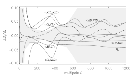
FIG. 10.: Derivative along flattest direction of the CI+NID distribution (dot-dashed) is decomposed into variations in the mode contributions, ${\langle\mbox{I,J}\rangle},$ and the overall spectral index $n_{s}$. The shaded region corresponds to the uncertainty of the WMAP measurement including cosmic variance.

	AD	AD+ISO	AD+ISO
	CMB+LSS	CMB	CMB+LSS
$\omega_{b}$	$0.023\pm 0.001$	$0.043\pm 0.006$	$0.041\pm 0.006$
$\omega_{c}$	$0.120\pm 0.006$	$0.11\pm 0.02$	$0.12\pm 0.01$
$\Omega_{\Lambda}$	$0.71\pm 0.03$	$0.79\,$${}^{+\,0.05}_{-\,0.07}$	$0.74\pm 0.03$
$n_{s}$	$0.97\pm 0.03$	$1.13\pm 0.07$	$1.10\pm 0.06$
$\tau$	$0.13\,$ ${}^{+\,0.08}_{-\,0.06}$	$0.21\,$${}^{+\,0.06}_{-\,0.08}$	$0.22\pm 0.07$
$\beta$	$0.50\pm 0.05$	$\hskip 7.11317pt\cdots$	$0.35\pm 0.05$
$z_{\langle\mbox{AD,AD}\rangle}$	1.0	$0.55\,$${}^{+\,0.16}_{-\,0.14}$	$0.61\pm{0.15}$
$z_{\langle\mbox{CI,CI}\rangle}$	$\hskip 7.11317pt\cdots$	$0.23\,$${}^{+\,0.11}_{-\,0.09}$	$0.23\pm 0.11$
$z_{\langle\mbox{NID,NID}\rangle}$	$\hskip 7.11317pt\cdots$	$0.28\,$${}^{+\,0.12}_{-\,0.10}$	$0.30\pm 0.12$
$z_{\langle\mbox{NIV,NIV}\rangle}$	$\hskip 7.11317pt\cdots$	$0.34\pm 0.14$	$0.28\,$${}^{+\,0.14}_{-\,0.11}$
$z_{\langle\mbox{AD,CI}\rangle}$	$\hskip 7.11317pt\cdots$	$-0.14\pm 0.10$	$-0.12\,$${}^{+\,0.12}_{-\,0.10}$
$z_{\langle\mbox{AD,NID}\rangle}$	$\hskip 7.11317pt\cdots$	$0.12\,$${}^{+\,0.09}_{-\,0.11}$	$0.11\,$${}^{+\,0.10}_{-\,0.12}$
$z_{\langle\mbox{AD,NIV}\rangle}$	$\hskip 7.11317pt\cdots$	$0.22\pm 0.10$	$0.19\pm 0.11$
$z_{\langle\mbox{CI,NID}\rangle}$	$\hskip 7.11317pt\cdots$	$-0.15\pm 0.10$	$-0.18\pm 0.10$
$z_{\langle\mbox{CI,NIV}\rangle}$	$\hskip 7.11317pt\cdots$	$-0.10\,$${}^{+\,0.10}_{-\,0.08}$	$-0.09\pm 0.08$
$z_{\langle\mbox{NID,NIV}\rangle}$	$\hskip 7.11317pt\cdots$	$0.17\pm 0.07$	$0.16\pm 0.08$
$z_{\mbox{ISO}}$	$\hskip 7.11317pt\cdots$	$0.84\pm^{0.08}_{0.13}$	$0.79\pm^{0.09}_{0.13}$
$f_{\mbox{ISO}}$	$\hskip 7.11317pt\cdots$	$0.60\pm^{0.09}_{0.11}$	$0.57\pm 0.09$
$\Omega_{m}$	$0.29\pm 0.03$	$0.21\pm^{0.07}_{0.05}$	$0.26\pm 0.03$
$h$	$0.70\pm 0.03$	$0.85\pm^{0.06}_{0.08}$	$0.80\pm 0.05$
$b$	$0.95\pm 0.08$	$\hskip 7.11317pt\cdots$	$1.3\pm 0.2$

TABLE IV.: Adiabatic plus all three isocurvature modes. The same conventions are used as in Table II, for mixed models with all three correlated isocurvature modes (AD+ISO). Results are included for both CMB and CMB+LSS datasets, and for pure adiabatic models (AD) for comparison.

In Fig. 12 we plot the CMB and matter power spectra for an adiabatic model and a mixed model with high likelihood, with parameters ($\omega_{b}$, $\omega_{c}$, $\Omega_{\Lambda}$, $n_{s}$, $\tau$, $\beta$, $f_{\mbox{ISO}}$) =(0.041, 0.13, 0.75, 1.06, 0.28, 0.37, 0.60). The adiabatic and mixed model spectra are essentially indistinguishable, despite the adiabatic mode contributing only $40\%$ of the total rms power of the mixed model spectra.

Although the posterior distributions for mixed models and pure adiabatic models hardly overlap, the high-likelihood models are connected in parameter space. That is to say, the goodness-of-fit, $\chi^{2},$ changes almost monotonically over a variation of parameters that interpolates linearly between these models, as shown in Fig. 13. This means that the posterior distribution is not bimodal but rather flat between the high likelihood adiabatic model and the high likelihood mixed model. A principal component analysis of the covariance matrix of the distribution, calculated about the high likelihood mixed model shown in Fig. 12, indicates that the flattest direction ${\bf y}_{0}$ has an uncertainty greater than $100\%$, with three eigen-directions having uncertainties greater than 50%.

FIG. 11.: Posterior distributions for Adiabatic plus CI+NID+NIV. The distributions for models with correlated adiabatic and three isocurvature modes are shown, using the CMB only (dashed) and (CMB+LSS) (solid). Where relevant the posterior for the pure adiabatic models (dot-dashed) is shown for comparison.

FIG. 12.: Power spectra of best-fit mixed models for three isocurvature modes. The angular power spectrum of CMB anisotropies, $C^{T}_{\ell},$ the temperature-polarization cross correlation spectrum, $C^{TE}_{\ell},$ and the galaxy power spectrum, $P(k),$ for the best-fit adiabatic model (dashed line) and best-fit mixed model with $f_{\mbox{ISO}}=60\%$ (solid line), with the auto-correlation contributions to the mixed model included. The CMB data points are overplotted and the sizes of the 2dFGRS error bars are indicated.

To elucidate what physical effects are responsible for these flat directions, we search for degenerate directions that arise from smaller subsets of the full parameter set. We have identified two such flat directions. The first is the degenerate direction described in Section III A involving seven parameters, which is again present here. This flat direction accounts for the negative correlations, $z_{\langle\mbox{AD,CI}\rangle}$ and $z_{\langle\mbox{CI,NID}\rangle},$ and the positive correlation $z_{\langle\mbox{AD,NID}\rangle}$. By performing a principal component analysis of these seven parameters, we find a very similar flat direction to the one shown in Fig. 10.

The second flat direction, that involves four parameters, is associated with a large shift in the value of the baryon density. By studying the two-dimensional marginalised distributions shown in Fig. 14, it is clear that the spectral index and the adiabatic and neutrino isocurvature velocity mode contributions are strongly correlated with the baryon density. Performing a principal component analysis of the covariance matrix of this four-parameter set, reveals a flat direction with an uncertainty of $50\%$. This cancellation is illustrated in Fig. 15, where the baryon density is increased by 8%, leading to the suppression (boosting) of even (odd)-numbered adiabatic acoustic peaks. This shift is compensated by increasing the power in the NIV mode by 29%, reducing that in the AD mode by 13% and increasing the overall spectral index $n_{s}$ by 2%, leaving the CMB temperature spectra unchanged to within the WMAP experimental error bars. It is not surprising that the neutrino velocity mode provides the oscillatory cancellation as the baryon density increases, given that it is approximately in phase with the adiabatic mode.

We now consider the statistical significance of these results. The mixed model reduces the total $\chi^{2}$ by 5. Under the approximation of a linear parametric dependence (which in this case is probably not a very good approximation), one would expect the reduction in $\chi^{2}$ to be governed by a $\chi^{2}$ distribution with nine degrees of freedom (i.e., equal to the number of extra parameters). Consequently, a reduction by only 5 where simply fitting the noise would lead to a reduction by 9, does not constitute evidence in favor of adding the extra parameters.

FIG. 13.: $\chi^{2}$ for models connecting adiabatic and mixed models, calculated along a path connecting the best-fit adiabatic model ${\bf x}_{1}$ with the best-fit mixed model ${\bf x}_{2}$, calculated at position ${\bf x}=\lambda{\bf x}_{2}+(1-\lambda){\bf x}_{1}$.

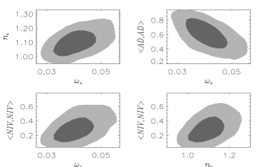
FIG. 14.: Two dimensional marginalized distributions. Correlations between the baryon density $\omega_{b}$, the spectral index $n_{s}$ and the contributions of the pure adiabatic and neutrino velocity isocurvature modes are illustrated. $\langle\mbox{I,J}\rangle$ denotes $z_{\langle\mbox{I,J}\rangle}$.

We conclude that although our results demonstrate that the data allows for large amounts of isocurvature, we have not found any evidence indicating that the models with more parameters offer a statistically significantly better fit. The same analysis may be applied to the additions of a single mode and pairs of modes. Adding a single mode adds two parameters, and we find a reduction of the total $\chi^{2}$ by 1 for the NIV mode, and less than 1 for the CI and NID modes. In none of these cases is the improvement in fit statistically significant. Similarly, for pairs of modes, five parameters are added, and the total $\chi^{2}$ decreases by approximately 1, 1, and 2 for the combinations CI+NID, CI+NIV, and NID+NIV, respectively.

It is possible in principle that a statistically significant improvement in fit might be obtained if the exponents in the power laws for the various modes were allowed to vary independently and/or additional effects such as tensor modes were allowed. We did not investigate this possibility.

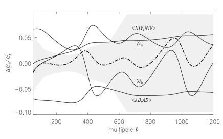
FIG. 15.: Degenerate direction in $\omega_{b}$, $n_{s}$, $A_{\langle\mbox{AD,AD}\rangle}$, and $A_{\langle\mbox{NIV,NIV}\rangle}$ The total derivative along the flattest degenerate direction (dot-dashed) is decomposed into variations in the four parameters above (all solid), which cancel to within the limits allowed by WMAP error bars (shaded).

IV Sensitivity of posterior distributions to constraints and prior distributions.

The results of the previous section were obtained using Bayes’ theorem

$$P_{posterior}(\alpha_{par}|{\bf x}_{data})\propto L({\bf x}_{data}|{\bf\alpha}_{par})~{}P_{prior}(\alpha_{par}),$$ (24)

where $\alpha_{par}$ spans the parameter space of models and $L({\bf x}_{data}|{\bf\alpha}_{par})$ is the likelihood of the model labeled by ${\bf\alpha}_{par}$ given the CMB (or CMB+LSS) data indicated by ${\bf x}_{data}$, subject to the prior distribution over the space of models $P_{prior}(\alpha_{par}).$ The posterior distribution is computed using MCMC techniques outlined in [25] and references therein. Certain prior distributions in the form of constraints, such as the positivity of various parameters that physically cannot be negative or the positive definiteness of the matrix-valued power spectrum, do not merit discussion. For most parameters uniform priors were assumed, following customary practice.

In this section we investigate the sensitivity of our conclusions (i.e., the posterior probability distribution) for those variables for which the choice of prior was important. In particular, we investigate the sensitivity to: (1) The allowed range for the reionization optical depth $\tau,$ (2) the priors for the redshift distortion parameter $\beta=b/\Omega^{0.6}$ and the bias $b,$ (3) the prior for $\omega_{b},$ that is whether a uniform prior is employed or whether information from other independent determinations of $\omega_{b}$ based on nucleosynthesis are employed, and (4) the choice of parameterization (or measure) for $A_{IJ}(k).$ In all cases we consider the $N=4$ example, including all possible isocurvature modes.

A Alternative Priors for Cosmological Parameters

1 Constraint on optical depth

Following the WMAP team analysis[8] of pure adiabatic models, we limited the reionization optical depth to the range $0\leq\tau<0.3$. When isocurvature modes were included, in particular the NIV mode, we observed that the distribution for $\tau$ seemed to concentrate toward the endpoint at $\tau=0.3.$ To investigate the sensitivity to the value of this cutoff, we considered an alternative upper limit at $\tau=0.5$. Fig. 16 compares the posterior distributions for these two upper bounds, showing those parameters for which the difference is greatest. Even with the upper bound raised to $\tau=0.5$ the posterior distribution still accumulates there. However, the effect on other parameters is mild, with only a slightly larger isocurvature contribution at $f_{\mbox{ISO}}=0.60\pm 0.10$ permitted.

FIG. 16.: Effect of changing the upper limit for $\tau$ from 0.3 (solid) to 0.5 (dashed). Only the posterior distributions for parameters where the difference is significant are shown; the distributions for the remaining parameters are unchanged from their $\tau<0.3$ values.

2 Priors from galaxy redshift survey data

We have included data on the galaxy power spectrum from the 2dFGRS survey, incorporating a Gaussian prior for the redshift distortion parameter with $\beta=0.43\pm 0.077,$ that is derived from a measurement of the redshift distortion effect observed in the galaxy survey [32, 31]. The WMAP team [8] have argued for an independent prior on the bias of $b=1.04\pm 0.11,$ obtained by computing the bispectrum of the 2dFGRS survey [35]. In the previous section we did not impose this prior on the bias since it was obtained under the assumption of Gaussian initial fluctuations. Furthermore, an implicit prior is placed on $\Omega_{m}$ (and therefore $\Omega_{\Lambda}$) when it is combined with the prior on $\beta$. We found a higher value for the bias, $b=1.3\pm 0.2$, obtained from constraining three isocurvature modes with the CMB+LSS dataset. A larger bias generally allows for a larger isocurvature fraction, so we now include the additional determination of $b$ to determine its effect on the allowed isocurvature contributions. The effect is small, with parameter value distributions virtually the same and the isocurvature contribution decreasing only slightly from $f_{\mbox{ISO}}=0.57$ to $0.53$.

We have also investigated the role of the prior on $\beta$ in constraining the ratio of the galaxy power spectrum to the matter power spectrum, $f(b,\beta)$. By relaxing the prior on $\beta$, we allow $f$ to vary freely so that only information on the shape of the power spectrum is utilised. The resulting parameter distributions are shown in Fig. 17, where $f$ has been optimised at each step in the chain. We observe that larger isocurvature fractions, $f_{\mbox{ISO}}=0.65\pm 0.09$ are allowed. In particular the NIV mode contribution increases to $z_{\langle\mbox{NIV,NIV}\rangle}=0.40\pm 0.15$. We have shown that such an increase is correlated with a reduction in the amplitude of the adiabatic mode. Such models were previously disfavoured by the prior on $\beta$ because of their resulting low matter power spectrum amplitudes, but are permitted when the normalisation of the matter power spectrum is free to vary. More models along the flat NIV direction are explored, thereby permitting larger values of $n_{s}$ and $\omega_{b}$. We also observe weaker constraints on $\omega_{c}$ and $\Omega_{\Lambda}$. This test demonstrates that the redshift distortion measurement is very informative.

FIG. 17.: Effect of discarding LSS amplitude information. Marginalized parameter distributions obtained using only the shape information from the LSS data (dashed) compared to those distributions obtained using the prior $\beta=0.43\pm 0.077$ (solid).

3 Prior on baryon density

In the previous section, when three possibly correlated isocurvature modes were allowed, we found $\omega_{b}=0.041\pm 0.006$ for the baryon density, a value discrepant with nucleosythesis based determinations of $\omega_{b},$ which indicate $\omega_{b}=0.022\pm 0.002$ [33]. We investigate the effect of replacing the uniform prior on $\omega_{b}$ with a prior that incorporates this complementary information. Fig. 18 shows the posterior distributions with and without the nucleosythesis determination. The median values and 68% confidence levels are shown in Table V. The posterior for the baryon density overlaps with the prior nucleosythesis distribution but values as large as $\omega_{b}=0.030$ are still permitted. There is a large reduction in the isocurvature contribution, in particular the NIV mode and its correlations, with the overall non-adiabatic fraction reduced to a median value of $f_{\mbox{ISO}}=0.31$. The cosmological parameters correlated with the NIV amplitude, such as $n_{s}$, $\tau$ and $\beta$ shift back toward their pure adiabatic values.

	CMB+LSS	CMB+LSS
	(BBN)	(standard)
$\omega_{b}$	$0.026\pm 0.002$	$0.041\pm 0.006$
$\omega_{c}$	$0.116\pm 0.008$	$0.12\pm 0.01$
$\Omega_{\Lambda}$	$0.71\pm 0.03$	$0.74\pm 0.03$
$n_{s}$	$0.99\pm 0.04$	$1.10\pm 0.06$
$\tau$	$0.12^{+0.07}_{-0.05}$	$0.22\pm 0.07$
$\beta$	$0.43\pm 0.05$	$0.35\pm 0.05$
$z_{\langle\mbox{AD,AD}\rangle}$	$0.91\,$${}^{+\,0.05}_{-\,0.08}$	$0.61\pm{0.15}$
$z_{\langle\mbox{CI,CI}\rangle}$	$0.13\,$${}^{+\,0.10}_{-\,0.07}$	$0.23\pm 0.11$
$z_{\langle\mbox{NID,NID}\rangle}$	$0.14^{+0.10}_{-0.06}$	$0.30\pm 0.12$
$z_{\langle\mbox{NIV,NIV}\rangle}$	$0.08\,$${}^{+\,0.06}_{-\,0.04}$	$0.28\,$${}^{+\,0.14}_{-\,0.11}$
$z_{\langle\mbox{AD,CI}\rangle}$	$-0.06\pm 0.11$	$-0.12\,$${}^{+\,0.12}_{-\,0.10}$
$z_{\langle\mbox{AD,NID}\rangle}$	$0.0008\pm 0.11$	$0.11\,$${}^{+\,0.10}_{-\,0.12}$
$z_{\langle\mbox{AD,NIV}\rangle}$	$0.06\pm 0.09$	$0.19\pm 0.11$
$z_{\langle\mbox{CI,NID}\rangle}$	$-0.10\pm 0.09$	$-0.18\pm 0.10$
$z_{\langle\mbox{CI,NIV}\rangle}$	$-0.003\pm 0.04$	$-0.09\pm 0.08$
$z_{\langle\mbox{NID,NIV}\rangle}$	$0.04\pm 0.05$	$0.16\pm 0.08$
$z_{\mbox{ISO}}$	$0.41\pm 0.14$	$0.79\pm^{0.09}_{0.13}$
$f_{\mbox{ISO}}$	$0.31\pm 0.09$	$0.57\pm 0.09$
$\Omega_{m}$	$0.29\pm 0.03$	$0.26\pm 0.03$
$h$	$0.70\pm 0.04$	$0.80\pm 0.05$
$b$	$1.1\pm 0.1$	$1.3\pm 0.2$

TABLE V.: Effect of incorporating the nucleosynthesis determination of $\omega_{b}.$ Median parameter values and $68\%$ confidence intervals as in Table II for mixed models with a nucleosynthesis prior (BBN, 1st column), compared to the standard results with a broad uniform prior (2nd column). The CMB+LSS dataset is used throughout.

FIG. 18.: Effect of incorporating the nucleosynthesis determination of $\omega_{b}.$ The curves show the posterior distributions from the CMB+LSS data with a flat prior for $\omega_{b}$ (shown in solid) and a Gaussian prior reflecting the determination $\omega_{b}=0.022\pm 0.002$ (shown as dashed).

B Dependence on mode parameterization

We examine the sensitivity of the posterior distribution to the choice of prior distribution for the coefficients of the matrix ${\cal A}_{IJ}=A_{IJ}~{}k^{n_{S}}.$ As detailed in section IIB, after normalizing the modes according to their contribution to the total CMB power from $\ell=2$ through $\ell=2000,$ we parameterized $A_{IJ}$ as $A_{IJ}\propto z_{IJ}$ where the constraint $\|z\|=1$ was imposed and the uniform spherical measure on the resulting sphere was assumed. A uniform prior for the constant of proportionality was assumed.

We now consider directly sampling a uniform distribution in the coefficients $A_{IJ}.$ This alternative prior makes a large difference for the case of three isocurvature modes, for which the allowed isocurvature rises from $f_{\mbox{ISO}}=0.57$ with the old prior to $f_{\mbox{ISO}}=0.81$ with the new prior. The posterior distributions are modified significantly, as indicated in Fig. 19.

We can understand this effect by observing that the constant of proportionality in eqn. 7, which we now label $A^{\prime}$, can be written as $(\sum_{IJ}A_{IJ}^{2})^{1/2}.$ Under this new parameterization where we sample uniformly in $A_{IJ}$, we therefore replace the uniform prior on ${A^{\prime}}$ with a prior so that $P(A^{\prime})\propto(A^{\prime})^{\alpha}$ where $\alpha=N(N+1)/2-1.$ This favours models with high values for ${A^{\prime}}$, corresponding to those with large positive and negative isocurvature contributions $A_{IJ},$ which may cancel out to fit the data. As discussed in the previous section, such models may be formed by moving along a degenerate direction consisting of the auto- and cross-correlations formed by the CI and NID modes with the adiabatic mode, and the spectral index $n_{s}.$ A similar direction was illustrated in Fig. 10. These models account for the increased contribution of both the CI and NID mode auto- and cross-correlations, and hence the reduction of the relative AD and NIV mode contributions. While the likelihood of such models with very high isocurvature is relatively low, the phase-space effect due to the modified prior boosts their posterior probability.

FIG. 19.: Alternative prior uniform in the coefficients $A_{IJ}.$ The posterior distributions with this new prior (dashed) are compared to those of the ‘standard’ prior described in Section II (solid).

FIG. 20.: Effect of reweighting to correct for bias against pure models. The left panel shows what posterior for the adiabatic mode contribution $z_{\langle\mbox{AD,AD}\rangle}$ would be in the absence of data. In the center panel we show how the posterior (from the prior in section IIB) (dashed) shifts (to the solid) curve) from a re-weighting that would give a flat posterior in the absence of data. The right panel shows the corresponding shift in $\omega_{b}$ resulting from the same reweighting.

Both of the previous priors disfavor models where any one mode dominates over the others. This is because of the product factor in the distribution given in eqn. (18). For the prior presented in section IIB, taking the limit $z_{\langle\mbox{AD,AD}\rangle}\to 1$ causes one of the eigenvalues of $z_{IJ}$ to approach one while the other $(N-1)$ eigenvalues approach zero. More quantitatively, if $z_{\langle\mbox{AD,AD}\rangle}=1-\epsilon^{2},$ the $(N-1)$ small eigenvalues cluster within $\epsilon$ of zero, giving a factor proportional to $\epsilon^{N(N-1)/2}$ in the product in eqn. (18). This gives a prior density for $z_{\langle\mbox{AD,AD}\rangle},$ marginalized with respect to the other parameters, proportional to $\epsilon^{N(N-1)/2-1}$ in the neighborhood of $z_{\langle\mbox{AD,AD}\rangle}.$ Consequently, even if the data indicated that all models where equally likely—that is, if the data was non-informative—our posterior would have a zero of the same order at the endpoint $z_{\langle\mbox{AD,AD}\rangle}=1$!

We may correct for such bias, or estimate its effect, by rescaling the prior so that in the absence of data the posterior in $z_{\langle\mbox{AD,AD}\rangle}$ would be flat, as shown in Fig. 20. The left panel shows the posterior for $z_{\langle\mbox{AD,AD}\rangle}$ in the absence of data for $N=4$ (i.e., adiabatic + three isocurvature modes). In the middle panel the (dashed) curve shows the posterior for the prior of section IIB. When this is rescaled (by dividing by the posterior with no data and then renormalizing) the posterior represented by the solid curve results. The right panel shows the results of this reweighting on $\omega_{b}.$ With this re-weighting the adiabatic fraction increases to $z_{\langle\mbox{AD,AD}\rangle}=0.87^{+0.08}_{-0.14}$, with a lower isocurvature fraction, $f_{\mbox{ISO}}=0.36\pm 0.12.$

V Discussion

We have presented a framework within which to consider correlated mixtures of adiabatic and isocurvature perturbations and to obtain simultaneously more model independent constraints on cosmological parameters as determined from CMB and large-scale structure datasets. Applying these methods to recent CMB data, from WMAP and several small-scale experiments, indicates that current constraints on a single correlated isocurvature mode are strong ($\approx 10\%$). These limits, however, degrade substantially when two or three correlated isocurvature modes are allowed, with non-adiabatic fractions as large as $60\%$ possible. Including large-scale structure data from the 2dF survey only slightly modifies these constraints.

The parameters significantly modified by including correlated isocurvature initial conditions are $\omega_{b},\tau,\beta$ and $n_{s},$ with the values of the baryon density values twice as large as in the pure adiabatic case not ruled out. These parameters are strongly correlated with the isocurvature amplitudes and for the current data are in fact degenerate along a well-defined direction in parameter space. Consequently, the likelihood function is not strongly peaked around a given model but relatively flat in a region interpolating between a set of mixed models and the pure adiabatic model. For many of the allowed models the large isocurvature fraction did not necessarily accompany a substantial decrease in the adiabatic power. This is possible because of interference phenomena as we explained. While we find that large isocurvature fractions are allowed we do not find evidence that the inclusion of such modes provides a statistically significant better fit to the present data.
Acknowledgments: K.M. and J.D. acknowledge the support of PPARC. M.B. thanks Mr D. Avery for financial support. P.G.F. thanks the Royal Society. C.S. is supported by a Leverhulme trust grant. We thank R. Durrer, U. Seljak, D. Spergel and R. Trotta for useful discussions.

A Rapid computation of cosmological models using DASh

1 Motivation and Description

Cosmological parameter estimation currently requires calculating at least $10^{6}$ models when a typical 6-dimensional parameter space is sampled uniformly. Using an MCMC sampler, which favors the region of high likelihood, reduces the number of computed models to $\approx 10^{4}$ for the same parameter space. Future parameter estimation studies will aim to measure many more parameters as the quality of CMB temperature and polarisation data improves, thereby increasing the computational cost. By including non-adiabatic initial conditions in this study, we have enlarged the parameter space to 16 dimensions, requiring computing many more models. The development of software that speeds up model computation is crucial for sampling such large parameter spaces.

Current codes take between 30 and 60 seconds to compute a single model, which is prohibitively long for sampling a large dimensional parameter space. One requires a method that both improves the precision of the computed $C_{\ell}$ spectrum as data becomes more accurate without sacrificing speed. The method adopted here and extended is the Davis Anisotropy Shortcut (DASh) [26]. With DASh, the accuracy depends primarily on the fineness of the grid, which depends on the size of available fast memory. Consequently, accuracy may be increased without sacrificing speed.

DASh was initially developed as a fast method for predicting the angular power spectrum given a set of cosmological parameters (the physical baryon density $\omega_{b}$, physical matter density $\omega_{m}$, relative cosmological constant density $\Omega_{\Lambda}$, relative curvature density $\Omega_{K}$ and reionization optical depth $\tau$) and an arbitrary primordial power spectrum. The method relied on the construction of grids: a low-$\ell$ grid

$${\cal G}_{\ell}^{L}[w_{b},w_{m},\Omega_{\Lambda},\Omega_{K}],\qquad 2\leq\ell\leq\ell_{t}$$

for an upper threshold $\ell_{t}[\Omega_{\Lambda},\Omega_{K}]$; a high-$\ell$ grid,

$${\cal G}_{\ell}^{H}[w_{b},w_{m}],\qquad\ell>\ell_{t};$$

a polarization grid

$${\cal G}_{\ell}^{P}[w_{b},w_{m}];$$

and a reionization grid

$${\cal G}_{\ell}^{R}[w_{b},w_{m},\tau],\qquad 2\leq\ell\leq\ell_{R}$$

for an upper threshold $\ell_{R}$. At each vertex of the low-$\ell$ and high-$\ell$ grids the temperature transfer function $\Delta_{\ell}^{T}(k)$ was pre-computed and stored. Similarly, for the polarization grid the polarization transfer functions, $\Delta_{\ell}^{E}(k),$ were pre-computed and stored. For the reionization grid, a function of $C_{\ell}^{T}[\tau]$ and $C_{\ell}^{T}[\tau=0]$ was stored at each grid point. After the initial construction of the grids, an arbitrary $C_{\ell}$ spectrum could be calculated in roughly 1 to 2 seconds, as long as its parameters were within the parameter range of the grid.

The $C_{\ell}^{T}$, $C_{\ell}^{TE},$ and $C_{\ell}^{E}$ spectra were calculated by interpolating the transfer functions, $\Delta_{\ell}^{T}(k)$ and $\Delta_{\ell}^{E}(k)$ from the values at the nearest vertices on the relevant grids. A linear interpolation of the quantities, $|\Delta_{\ell}^{T}(k)|^{2}$, $\Delta_{\ell}^{T}(k)\Delta_{\ell}^{E}(k)$ and $|\Delta_{\ell}^{E}(k)|^{2}$ was performed before integrating over $k$ to obtain the low $C_{\ell}^{T}$ spectrum, and the high $C_{\ell}^{T}$, $C_{\ell}^{TE}$ and $C_{\ell}^{E}$ spectra for $\tau=0$. The high $C_{\ell}^{T}$, $C_{\ell}^{TE}$ and $C_{\ell}^{E}$ spectra were then rescaled in $\ell$ to take into account the modified angular diameter distance to recombination. The low and high $\ell$ temperature spectra were then combined to obtain the $C_{\ell}^{T}$, $C_{\ell}^{TE}$ and $C_{\ell}^{E}$ spectra for $\tau=0$. The final spectrum was calculated by multiplying by a reionization correction envelope obtained from the reionization grid for $\ell\leq\ell_{R}$ and a suppression factor $e^{-2\tau}$ for $\ell>\ell_{R}$ in the temperature case. For the temperature-polarization cross-correlation and polarization auto-correlation, a fitting function for the reionization bumps was used. More details of the initial release [27] of DASh can be found in [26]. Current alternative methods to perform rapid CMB model computation or to sample parameter space rapidly include [36] and [37].

FIG. 21.: The different terms in the Line-of-Sight integral (eqn. A8) separated into ones that are positive [left] and negative [right] in the limit $k\rightarrow 0$. The positive terms are : $\dot{\alpha}$ (solid), $\delta_{\gamma}$ (dotted), $\frac{\dot{\theta}_{b}}{k^{2}}$ (dashed) and $\frac{\ddot{\Pi}}{k^{2}}$ (long dashed). The negative terms are : $\dot{\eta}$ (solid), $\alpha$ (dotted), $\ddot{\alpha}$ (dashed), $\frac{\theta_{b}}{k^{2}}$ (long dashed), $\frac{\dot{\Pi}}{k^{2}}$ (dot-dashed), $\frac{\Pi}{k^{2}}$ (dot-long dashed) and $\Pi$ (short-long dashed). Clearly $\delta_{\gamma}$, $\dot{\eta}$ and $\Pi$ are finite ($\propto k$) as $k\rightarrow 0$ whereas the rest diverge as $\frac{1}{k}$.

2 Code extensions

We extended the initial DASh version by including all isocurvature modes as in [12]. In the new version, the low-$\ell$, high-$\ell$ and polarization grids were created for each pure mode. The cross-correlations between modes were calculated at the interpolation stage. We have replaced the fitting functions for the reionization bumps with two more reionization grids in $C_{\ell}^{TE}$ and $C_{\ell}^{E},$ for greater accuracy and because the isocurvature mode bumps had very different shapes to the adiabatic mode bumps. The three reionization grids were therefore calculated for the auto-correlation and cross-correlation modes.

We have also added the pre-computation of a matter transfer function $T(k)$ grid

$${\cal G}^{T}(k)[\omega_{b},\omega_{m}]$$

for each pure mode with $\Omega_{\Lambda}=0.6$ for the range in $k$ space covered by the 2dFGRS dataset [7]. The matter power spectrum was then computed by interpolating $T(k)$ for each mode, multiplying by the ratio of growth functions for $\Omega_{\Lambda}\neq 0.6$ and finally obtaining $P(k)$ by summing over modes. The computation of a single $P(k)$ is virtually instantaneous (after pre-computation of the grid).

Finally, due to the ${1}/{k}$ divergences that appear in some terms (e.g., the Newtonian potentials) of the line-of-sight (LOS) integral [38] for the NIV mode, special care must be taken when pre-computing the grids, as this introduces a numerical error as large as $5\%$ to $10\%$ for $\ell<10$ which could be amplified to as much as $50\%$ after the interpolation. We discuss these details next.

3 Neutrino isocurvature velocity mode

For the neutrino isocurvature velocity mode, the Newtonian potentials which are defined in the conformal Newtonian gauge (see for example [39]), diverge as ${1}/{k}$ and ${1}/{t}$ where $t$ denotes conformal time. To first order they are

$$\Psi = -\frac{4R_{\nu}}{15+4R_{\nu}}\;\frac{1}{kt}+\ldots$$ (A1)

$$\Phi = +\frac{4R_{\nu}}{15+4R_{\nu}}\;\frac{1}{kt}+\ldots$$ (A2)

where $R_{\nu}$ is a constant defined in [12]. These divergences have created confusion in the past and have led some authors to discard this mode as unphysical. The singularities above, however, are coordinate singularities, and disappear in synchronous gauge. All physical observables such as $C_{\ell}$s are finite for the NIV mode.

         

FIG. 22.: Accuracy of the computation of the temperature transfer function. [Left] The temperature transfer function $\Delta_{2}(k)$ calculated using a Boltzmann code (solid), with the line-of-sight integral (dashed) and with the integration by parts (dotted). [Upper Right] The angular power spectrum $C_{\ell}$ for a Boltzmann code (solid), LOS (dashed) and by parts (dotted). [Lower Right] Percent difference between LOS and Boltzmann (solid) and by parts and Boltzmann (dashed).

Let $t_{0}$ be the conformal time today, $t_{i}$ an initial conformal time deep into the radiation era, $x\equiv k(t_{0}-t),$ and $g(t)=\dot{\tau}(t)e^{\tau(t)}$ the visibility function. The optical depth back to $t$ is defined as $\tau(t)=\int_{t_{0}}^{t}dt\;\;\dot{\tau}$. We use the conventions and perturbation variables of [39]; $h$ and $\eta$ are the synchronous metric perturbations, $\delta_{\gamma}$ the photon density contrast, $\theta_{b}$ the baryon velocity divergence, $\Pi=F_{2}+G_{0}+G_{2}$ the polarization source term with $F_{\ell}$ and $G_{\ell}$ the sum and difference of the two photon polarizations, and $\alpha\equiv\frac{1}{2k^{2}}(\dot{h}+6\dot{\eta})$ the gauge transformation variable. For the neutrino isocurvature velocity mode, at early times and on large scales the above variables are given to leading order in $t$ by

$$\delta_{\gamma}\propto kt+\ldots,\quad\theta_{b}\propto k+\ldots,\quad\eta\propto kt+\ldots,\quad$$ (A4)

$$\alpha\propto\frac{1}{k}+\ldots,\quad\Pi\propto kt+\ldots.$$ (A5)

The line-of-sight integral [38] for the temperature transfer function is given by

$$\Delta_{\ell}(k)= \int_{t_{i}}^{t_{0}}\;dt\;j_{\ell}(x)\;\Bigg{\{}\,e^{\tau}(\dot{\eta}+\ddot{\alpha})$$ (A8)

$$+\,g(t)\left[\frac{1}{4}\delta_{\gamma}+\frac{\dot{\theta}_{b}}{k^{2}}+2\dot{\alpha}+\frac{1}{16}\Pi\frac{3}{16k^{2}}\ddot{\Pi}\right]$$

$$+\,\dot{g}(t)\left[\frac{\theta_{b}}{k^{2}}+\alpha+\frac{3}{8k^{2}}\dot{\Pi}\right]+\ddot{g}(t)\frac{3}{16k^{2}}\Pi\Bigg{\}}$$

Most terms in the above equation diverge as ${1}/{k}$ as shown in Fig. 21. The transfer functions, $\Delta_{\ell}(k),$ however, are finite, since the Bessel functions are well approximated by $j_{\ell}(kt)\propto(kt)^{\ell}$ at small $k,$ which is sufficient to cancel the ${1}/{k}$ divergence. This means that if $\Delta_{\ell}(k)$ is calculated using an exact Boltzmann code, it will be finite. Using the LOS integral above, however, one should worry that in computing $\Delta_{\ell}(k)$ the divergent terms will cause numerical noise on large scales, because of the subtraction of large numbers of (nearly) equal magnitude. This indeed occurs, with resulting errors ranging from $5\%$ to $10\%$. Such errors are less a problem for codes based entirely on the LOS method because the errors lie below the cosmic variance. Using the DASh code, however, the interpolation between models with this type of random error boosts the final error to as much as $30\%$ to $50\%$ at $\ell<10$ in some cases.

In order to eliminate the above numerical error, one can integrate eqn. (A8) by parts, so that

$$\Delta_{\ell}(k)=\int_{t_{i}}^{t_{0}}\;dt\;\Bigg{\{} j_{\ell}(x)\;\left[e^{\tau}\dot{\eta}+\frac{1}{4}g(t)\left(\delta_{\gamma}+\frac{1}{4}\Pi\right)\right]$$ (A11)

$$+\,\frac{dj_{\ell}}{dx}\left[e^{\tau}k\dot{\alpha}+\,\dot{g}(t)\frac{3}{16k}\Pi\,\right.$$

$$\qquad+\,\left.g(t)\left(k\alpha+\frac{\theta_{b}}{k}+\frac{3}{16k}\dot{\Pi}\right)\right]\Bigg{\}}$$

A quick check demonstrates that all the terms in the above equation are finite as $k\rightarrow 0$, which gives stable and accurate results when integrated numerically. We compare the different integration methods in Fig. 22.

FIG. 23.: The temperature transfer functions $\Delta_{200}(k)$ calculated using the LOS method (dotted) and linear interpolation (solid). The prominent feature is a beat of much lower frequency than the transfer function. This is what limits the interpolation accuracy. (Note that the actual code in DASh interpolates between the squares of the transfer functions which decreases the effect of the beat).

4 Accuracy and Timing

The LOS method is an extremely accurate method and is limited only by the accuracy of the Bessel functions, which for flat models is $0.1\%$, as was also demonstrated in [40]. Indeed this is the accuracy of all the transfer functions computed in DASh. The approximation techniques introduce further errors, namely interpolation error for all models and approximation error on large scales for reionized models due to the approximate method used to include reionization effects on large scales.

The interpolation error is due to an intrinsic $0.1\%$ error of the transfer functions which is amplified by interpolation, and a beat phenomenon which arises because the frequencies of the transfer functions being interpolated are slightly offset from each other and the target function. The intrinsic interpolation error could be remedied if the transfer functions were calculated with an exact Boltzmann code, though this would be at a cost in speed of pre-computation. To illustrate the effect of the interpolation error we plot the calculated LOS transfer function and the interpolated one in Fig. 23. Note that the interpolation in Fig. 23 is between transfer functions and not their squares, as is actually done in DASh, to dramatize the effect. Interpolating the squares of the transfer functions reduces this error, at the expense of having to interpolate $3\times 10$ transfer functions (counting the temperature and polarization for all auto- and cross-correlation modes) instead of $2\times 4$ (where the cross-correlation modes are calculated after interpolation).

FIG. 24.: Maximum and RMS percentage differences between the DASh interpolated spectra and the line-of-sight computed spectra. Maximum (dashed) and RMS (solid) percentage differences of DASh compared to the Line-Of-Sight method. From left to right we show the CMB temperature spectrum, CMB polarization spectrum and matter power spectrum $P(k)$. From top to bottom we show the adiabatic, CDM isocurvature, neutrino isocurvature velocity and neutrino isocurvature density modes. The errors for $C_{\ell}$ were calculated using 2048 models and for $P(k)$ using 512 models (we excluded variation of $\tau$ for the matter power spectrum.

To check that the inclusion of additional initial conditions, and the extension to compute the matter power spectrum, were sufficiently accurate we tested the DASh code against $2048$ models sampled from a grid in $\{\omega_{b},\omega_{c},\Omega_{\Lambda},\tau\},$ in the case of CMB temperature and polarization, and $512$ models sampled from a grid in $\{\omega_{b},\omega_{c},\Omega_{\Lambda}\},$ in the case of the matter power spectrum. We plot the maximum and root-mean-square (rms) errors in Fig. 24 for all auto-correlation mode spectra. For the CMB temperature spectrum (for which the most accurate measurements exist) we see that the maximum error is less than 2% over a wide range in $\ell$, which is better than the WMAP measurement error. On large scales ($\ell<10$) the maximum error increases to 10% for some modes but this is still well below cosmic variance.

We tested the effect of these numerical errors on the likelihood computed for each model and found the measured difference to be negligibe.

The isocurvature-modified DASh described here took approximately 3–4 seconds on a 1GHz PentiumIII processor to compute the CMB temperature, polarization, and cross-correlation spectra as well as the matter power spectrum, for a single mode. The full matrix of 4 modes and their cross-correlations required approximately 15 seconds per model.

REFERENCES

- [1] C. Bennett et al., (WMAP collab), Astrophys. J. Supp. 148, 1 (2003); A. Kogut et al., Astrophys. J. Supp. 148, 161 (2003); G. Hinshaw et al., Astrophys. J. Supp. 148, 135 (2003).
- [2] WMAP: http://map.gsfc.nasa.gov/.
- [3] C. L. Kuo, et al., Astrophys. J. 600, 32 (2004).
- [4] J. Ruhl et al., Astrophys. J, 599, 786 (2003).
- [5] T. J Pearson et al., Astrophys. J. 591, 556 (2003).
- [6] P. F. Scott et al., Mon. Not. R. Astron. Soc. 341 1076 (2003).
- [7] W. J. Percival et al., Mon. Not. R. Astron. Soc. 327, 1297 (2001).
- [8] D. Spergel et al., Astrophys. J. Supp., 148, 175 (2003).
- [9] P. J. E. Peebles, Nature 327, 210 (1987); Astrophys. J. Lett. Ed. 315, L73 (1987); Astrophys. J. 510, 523 (1999); 510, 531 (1999).
- [10] J. R Bond and G. Efstathiou, Mon. Not. R. Astron. Soc. 22, 33(1987).
- [11] A. Rebhan & D. Schwarz, Phys. Rev. D 50, 2541 (1994); A. Challinor & A. Lasenby, Astrophys. J. 513, 1 (1999).
- [12] M. Bucher, K. Moodley and N. Turok, Phys. Rev. D. 62, 083508 (2000); Phys. Rev. Lett. 87, 191301 (2001).
- [13] D. Langlois, Phys. Rev D. 59, 123512 (1999).
- [14] T. Moroi & T. Takahashi, Phys. Lett. B 522, 215 (2001).
- [15] D. H. Lyth & D. Wands, Phys. Rev. Lett. B 524, 5 (2002).
- [16] J. Garcia-Bellido & D. Wands, Phys. Rev D 52, 6739 (1995); 53, 5437 (1996).
- [17] A. Linde and V. Mukhanov, Phys. Rev. D 56, 535, (1997).
- [18] C. Gordon, D. Wands, B. Basset & R. Maartens, Phys. Rev. D P63, 023506, (2000).
- [19] M. Bucher, K. Moodley & N. Turok, Phys. Rev. D 66, 023528 (2002).
- [20] E. Pierpaoli, J. Garcia-Bellido & S. Borgani, J. High. Energy. Phys. 10, 15 (1999); K. Enqvist & H. Kurki-Suonio, Phys. Rev. D 61, 043002 (2000); K. Enqvist, H. Kurki-Suonio & J. Valiviita, Phys. Rev. D 62, 103003 (2000); ibid, Phys. Rev. D65, 043002 (2002); L. Amendola et al., Phys. Rev. Lett. 88, 211302 (2002).
- [21] R. Trotta, A. Riazuelo & R. Durrer, Phys. Rev. Lett. 87, 231301 (2001); Phys. Rev. D 67, 063520 (2003).
- [22] H. V. Peiris et al., Astrophys. J. 148, 213 (2003); C. Gordon & A. Lewis, Phys. Rev. D 67 123513 (2003); J. Valiviita & V. Muhonen, Phys. Rev. Lett. 91, 131302 (2003); C. Gordon & K. A. Malik, astro-ph/0311102 (2003).
- [23] P. Crotty, J. Garcia-Bellido, J. Lesgourgues & A. Riazuelo, Phys. Rev. Lett. 91, 171301 (2003).
- [24] M. Bucher, J. Dunkley, P. G. Ferreira, K. Moodley & C. Skordis, in press, Phys. Rev. Lett., astro-ph/0401417 (2004).
- [25] J. Dunkley, M. Bucher, P. G. Ferreira, K. Moodley & C. Skordis, submitted, Mon. Not. R. Astron. Soc., astro-ph/0405462 (2004).
- [26] M. Kaplinghat, L. Knox & C. Skordis, Astrophys. J. 578, 665 (2002).
- [27] http://www.physics.ucdavis.edu/cosmology/dash/.
- [28] M. L. Mehta, Random Matrices (Boston: Academic Press, 1991).
- [29] X. Wang et al., Phys. Rev. D 68, 123001 (2003).
- [30] http://www.hep.upenn.edu/ max/
- [31] L. Verde et al., (WMAP collab.), Astrophys. J. Supp. 148 195 (2003).
- [32] J. A. Peacock et al., Nature 410, 169 (2001).
- [33] B. D. Fields & S. Sarkar, Phys. Rev. D 66 010001 (2002).
- [34] A. Reiss et al., Astron. Journ. 116, 1009 (1998); S. Perlmutter et al., Astrophys. J. 517, 565 (1999).
- [35] L. Verde et al., 2002, Mon. Not. R. Astron. Soc., 335, 432 (2002).
- [36] A. Kosowsky, M. Milosavljevic & R. Jimenez, Phys. Rev. D 66 063007 (2002).
- [37] H. B. Sandvik et al., astro-ph/0311544 (2003).
- [38] U. Seljak & M. Zaldarriaga, Astrophys. J. Supp. 469, 437 (1996).
- [39] C. P. Ma & E. Bertschinger, Astrophys. J. 455, 7 (1995).
- [40] U. Seljak et al., Phys. Rev. D 68 083507 (2003).