Correlated isocurvature perturbations from mixed inflaton-curvaton decay

Abstract

We study cosmological perturbations in the case that present-day matter consists of a mixture of inflaton and curvaton decay products. We calculate how the curvaton perturbations are transferred to its decay products in the general case when it does not behave like dust. Taking into account that the decay products of the inflaton can also have perturbations results in an interesting mixture of correlated adiabatic and isocurvature perturbations. In particular, negative correlation can improve the fit to the CMB data by lowering the angular power in the Sachs-Wolfe plateau without changing the peak structure. We do an 11-parameter fit to the WMAP data. We find that the best-fit is not the ’concordance model’, and that well-fitting models do not cluster around the best-fit, so that cosmological parameters cannot be reliably estimated. We also find that in our model the mean quadrupole ($l=2$) power is $l(l+1)C_{l}/2\pi=1081\mu$K², much lower than in the pure adiabatic $\Lambda$CDM model, which gives $1262\mu$K².

, ,

1 Introduction

The building blocks of what is today known as the curvaton model were introduced in [1, 2] (some early discussion can be found in [3, 4]). The first detailed application to the observed CMB anisotropies was done in [5], in the context of the pre-big bang scenario. The model was then applied to inflation in detail and given the name “curvaton” in [6, 7].

In the curvaton model the perturbations of the cosmic microwave background and large-scale structure originate from a field, the curvaton, which is different from the field(s) driving the dynamics of the very early universe, be it inflation, pre-big bang collapse or something else. In what follows, we adopt the language of single field inflation for describing the primordial universe, though our considerations could apply to other cosmological scenarios as well.

During inflation and reheating, the curvaton is assumed to be completely subdominant. The mass of the curvaton field is also assumed to be much less than the Hubble parameter during inflation, so that the curvaton field value is frozen, and the curvaton will acquire a spectrum of quantum fluctuations which become classical. After inflation, when the Hubble parameter falls and becomes of the order of the curvaton mass, the curvaton will start to oscillate around the minimum of its potential. Assuming the potential to be quadratic about the minimum, the energy density in the curvaton field, averaged over oscillations, decays like $a^{-3}$, where $a$ is the scale factor. Taking the universe after reheating to be dominated by radiation, the relative contribution of the curvaton to the energy density increases. (Since the curvaton field value and therefore energy density is constant before the start of the oscillations, its relative contribution increases even faster during that period.)

We assume that the curvaton decays into baryons, cold dark matter (CDM), leptons and photons. The leptons are assumed to consist of (or later decay into, depending on when the curvaton decays) electrons and neutrinos. (Electrons play no role in our discussion, and will not be mentioned from now on.) If the curvaton decays before it contributes to the background, the perturbations inherited by its decay products will be of the isocurvature type, whereas if the curvaton completely determines the background when it decays, the perturbations will be adiabatic. This conversion of isocurvature perturbations into adiabatic ones is the essence of the curvaton mechanism. If the curvaton decays between these two extremes, its decay products will inherit a mixture of correlated adiabatic and isocurvature perturbations [8]. This has been studied in [9, 10, 11, 12, 13, 14, 15, 16, 17].

In the present paper, we extend in two respects previous studies (building particularly on [16]) of the case that the curvaton decays while it contributes to the energy density but does not completely dominate it.

First, it has usually been assumed that one can treat the curvaton as a pressureless fluid in calculating its decay. However, as this description is valid only as an average over oscillations, one would not expect it to apply in the case of a rapid decay, or when the field decays just as it is starting to oscillate (recently studied in [17]). We will calculate the decay without this assumption, using the curvaton field equation, and will obtain the limit of validity of the dust approximation.

Second, it has usually been assumed that even when present-day radiation and matter consist of a mixture of inflaton and curvaton decay products, the inflaton decay products have no perturbations. We will take into account the possibility that both the inflaton and curvaton decay products carry some (uncorrelated) perturbations, resulting in an interesting mixture. This case has been studied in [7, 9, 17] and is also reminiscent of double inflation models [3, 18, 19, 20, 21, 22]. Two limiting cases are the usual inflaton scenario, where all present-day matter comes from the inflaton, and the original pre-big bang curvaton scenario [5], where everything comes from the curvaton.

In section 2 we consider the decay of the curvaton, solve the decay equations numerically and discuss recovering the dust approximation. In section 3 we fit our spectrum of perturbations to the measurements made by the WMAP satellite. We discuss the interesting features of the spectrum, in particular suppression of the low multipoles and negative running of the spectral index. Having two independent sources of perturbations allows for a spectrum where one can have different behaviour of the low and high multipoles. The acoustic peak structure can remain very close to the pure adiabatic case, while the angular power on the Sachs-Wolfe plateau can be much reduced, leading to better overall fit than the pure adiabatic $\Lambda$CDM model. We also find that the inclusion of isocurvature modes opens up the space of well-fitting models, so that one cannot determine the cosmological parameters from the WMAP data alone. A detailed study of the estimation of the isocurvature contribution and the cosmological parameters with our perturbation spectrum will be presented later [23].

2 The curvaton decay

2.1 The set-up

We assume that there is a bath of baryons, CDM, neutrinos and photons produced by the decay of the inflaton field. We take the perturbations in these fluids to be adiabatic, as expected from single field models of inflation [24]. We also assume that there is a curvaton field which is subdominant, but frozen at some field value so that its relative contribution to the energy density rises. The curvaton field is assumed to have a spectrum of perturbations, acquired during inflation, which is uncorrelated with that of the inflaton decay products.

Like the inflaton, the curvaton is assumed to decay into baryons, CDM, neutrinos and photons, which inherit the perturbations of the curvaton. The final state will therefore consist of a mixture of products of inflaton and curvaton decay, both with their own spectrum of perturbations.

We will follow the system numerically from the time that the curvaton is frozen and subdominant until the time it has completely decayed. We will see how the resulting spectrum of perturbations in the decay products depends on the initial conditions and parameters of the model. Our analysis of the decay is a generalisation of that in [16], where the curvaton decay was followed numerically assuming that the curvaton behaves as a pressureless fluid.

2.2 The equations

The background.

The spacetime is a perturbed Friedmann-Robertson-Walker universe. In accordance with the generic inflationary prediction, we take the background spacetime to be spatially flat. In the uniform curvature gauge, the metric reads (we consider only scalar perturbations)

$$\rmd s^{2}=-(1+2\phi)\rmd t^{2}+2aB_{,i}\rmd t\rmd x^{i}+a^{2}\delta_{ij}\rmd x^{i}\rmd x^{j}\ .$$ (1)

Throughout, we follow the notational conventions of [12, 16, 25], except that we prefer to use $\mathcal{R}$, the curvature perturbation on the comoving hypersurface, rather than $\zeta$, the curvature perturbation on the uniform energy density hypersurface. On superhorizon scales, the two are related by $\mathcal{R}=-\zeta$.

As sources, we have radiation ($r$), matter ($m$) and the curvaton field ($\sigma$). The relation between the background sources and geometry is given by

$$H^{2}=\frac{1}{3M_{Pl}^{2}}\rho$$ (2)

$$\dot{\rho}+3H(\rho+P)=0\ ,$$ (3)

where $H=\dot{a}/a$, $M_{Pl}=1/\sqrt{8\pi G_{\textrm{N}}}$ is the (reduced) Planck mass and $\rho$ and $P$ are the total energy density and pressure, respectively. In terms of the individual components, we have

$$\Sigma_{\alpha}\rho_{\alpha}=\rho\ ,\quad\Sigma_{\alpha}P_{\alpha}=P\ ,$$ (4)

where $\alpha=r,m,\sigma$. For radiation and matter we have $P_{r}=\frac{1}{3}\rho_{r},P_{m}=0$, so that if there was no energy transfer between the components, their energy densities would decay like $\rho_{r}\propto a^{-4}$ and $\rho_{m}\propto a^{-3}$. Since the curvaton decay transfers energy into radiation and matter, the behaviour of the energy densities is given instead by

$$\dot{\rho}_{\alpha}+3H(\rho_{\alpha}+P_{\alpha})=Q_{\alpha}\ ,$$ (5)

where $Q_{\alpha}$ is the energy density transfer per unit time to the fluid $\alpha$.

We take the curvaton field to be minimally coupled to gravity and to have the potential $V(\sigma)=\frac{1}{2}m^{2}\sigma^{2}$. We model the curvaton decay phenomenologically by introducing constant decay rates to both radiation and matter into the equation of motion, as in [16]. The curvaton equation of motion for the background then reads

$$\ddot{\sigma}+(3H+\Gamma)\dot{\sigma}+m^{2}\sigma=0\ ,$$ (6)

where $\sigma$ is the background value of the curvaton field and $\Gamma=\Gamma_{r}+\Gamma_{m}$ is the curvaton decay rate, with $\Gamma_{r}$ and $\Gamma_{m}$ being constants. Using this effective description of decay, we ignore the possibility of parametric resonance [26, 27], as is usually done for curvaton models. Thermal corrections to the potential and to the decay rate [28] could also be important, since the curvaton is coupled to the thermal bath of matter and radiation [29]; we ignore these too.

The energy density and pressure of the curvaton are given by

$$\rho_{\sigma}=\frac{1}{2}\dot{\sigma}^{2}+\frac{1}{2}m^{2}\sigma^{2}$$

$$P_{\sigma}=\frac{1}{2}\dot{\sigma}^{2}-\frac{1}{2}m^{2}\sigma^{2}\ ,$$ (7)

and the energy transfers are

$$Q_{r}=\Gamma_{r}(\rho_{\sigma}+P_{\sigma})$$

$$Q_{m}=\Gamma_{m}(\rho_{\sigma}+P_{\sigma})$$

$$Q_{\sigma}=-(\Gamma_{r}+\Gamma_{m})(\rho_{\sigma}+P_{\sigma})\ .$$ (8)

Note that $\rho_{\sigma}+P_{\sigma}=\dot{\sigma}^{2}$. In [16], it was noted that we have an upper limit $\Gamma_{m}/\Gamma_{r}\lesssim 10^{-6}$ from the requirement that the curvaton decay should be complete before big bang nucleosynthesis (BBN) at $z\sim 10^{10}$ and matter should be subdominant until the matter-radiation equality at $z\lesssim 10^{4}$. This limit only holds if all matter and radiation come from the curvaton, which is not true in our case (or in the case of [16]). We will discuss the limit on $\Gamma_{m}/\Gamma_{r}$ in section 2.4.

For comparison with the dust treatment of the curvaton in [16], let us define [30]:

$$\rho_{\sigma}+P_{\sigma}\equiv\left(\gamma+\gamma_{p}\right)\rho_{\sigma}\ ,$$ (9)

where $\gamma\rho_{\sigma}$ and $\gamma_{p}\rho_{\sigma}$ are the average and the periodic part, respectively, of $\rho_{\sigma}+P_{\sigma}$ over an oscillation. In the regime where the curvaton oscillation is much more rapid than the decay, $m\gg\Gamma$, we can neglect $\gamma_{p}$. Moreover, for a quadratic potential $\gamma=1$, so that in the rapid oscillation limit we approximately recover the expressions of [16]:

$$Q_{r}=\Gamma_{r}\rho_{\sigma}$$

$$Q_{m}=\Gamma_{m}\rho_{\sigma}\ .$$ (10)

However, we do not expect (2.2) to be a good approximation when the field does not oscillate rapidly when it decays.

The perturbations.

We are interested in the behaviour of perturbations only in the large-scale limit, when spatial gradients can be neglected. Then, the equations for the perturbations read (after eliminating the metric perturbation $\phi$) [12, 16]

$$\delta\dot{\rho}_{\alpha}+3H(\delta\rho_{\alpha}+\delta P_{\alpha})=\delta Q_{\alpha}-\frac{\delta\rho}{2\rho}Q_{\alpha}\ ,$$ (11)

where $\delta\rho_{\alpha},\delta P_{\alpha}$ and $\delta Q_{\alpha}$ are, respectively, the perturbation in the energy density and pressure of, and energy transfer to, the component $\alpha$. The total perturbation obeys the covariant conservation equation

$$\delta\dot{\rho}+3H(\delta\rho+\delta P)=0\ ,$$ (12)

where

$$\delta\rho=\Sigma_{\alpha}\delta\rho_{\alpha}\ ,\quad\delta P=\Sigma_{\alpha}\delta P_{\alpha}\ .$$ (13)

The equation of motion for the curvaton field perturbation $\delta\sigma$ is

$$\delta\ddot{\sigma}+(3H+\Gamma)\delta\dot{\sigma}+m^{2}\delta\sigma=\left(2m^{2}\sigma+\Gamma\dot{\sigma}\right)\frac{\delta\rho}{2\rho}+3H\dot{\sigma}\left(\frac{\delta P}{\delta\rho}-\frac{P}{\rho}\right)\frac{\delta\rho}{2\rho}\ .$$ (14)

The perturbations in the energy density and pressure of the curvaton are given by

$$\delta\rho_{\sigma}=\dot{\sigma}\delta\dot{\sigma}+m^{2}\sigma\delta\sigma+\frac{\delta\rho}{2\rho}\dot{\sigma}^{2}$$

$$\delta P_{\sigma}=\dot{\sigma}\delta\dot{\sigma}-m^{2}\sigma\delta\sigma+\frac{\delta\rho}{2\rho}\dot{\sigma}^{2}\ ,$$ (15)

and the perturbed energy transfers are

$$\delta Q_{r}=\Gamma_{r}(\delta\rho_{\sigma}+\delta P_{\sigma})$$

$$\delta Q_{m}=\Gamma_{m}(\delta\rho_{\sigma}+\delta P_{\sigma})$$

$$\delta Q_{\sigma}=-(\Gamma_{r}+\Gamma_{m})(\delta\rho_{\sigma}+\delta P_{\sigma})\ .$$ (16)

We have assumed that the decay rates are constant also at the perturbed level, as in [16].

2.3 Behaviour of the background

The parameters of the background are the curvaton mass $m$, the decay rate $\Gamma$, the ratio $\Gamma_{m}/\Gamma_{r}$, as well as the initial values which consist of the initial curvaton field value $\sigma_{0}$ and the initial radiation energy density $\rho_{r0}$. Under the assumption that matter is subdominant, the initial energy density of matter makes no difference. Since we assume that initially $H\gg m,\Gamma$, we see from (6) that the curvaton is essentially frozen at a constant value to which it has been driven during inflation, so its initial velocity is negligible (though non-zero). For the curvaton to be subdominant, we must have $\rho_{r0}\gg\frac{1}{2}m^{2}\sigma_{0}^{2}$.

When the Hubble parameter becomes of the order of the curvaton mass, $H\sim m$, the curvaton rolls down the potential and starts to oscillate. When the Hubble parameter becomes of the order of the decay rate, $H\sim\Gamma$, the curvaton decays into radiation and matter. However, since the energy transfer in (2.2) is proportional to $\dot{\sigma}^{2}$, there is no decay as long as the field is frozen. This means that if $m<\Gamma$, the decay will not start at $H\sim\Gamma$, but only later at $H\sim m$, when the field will simultaneously roll down the potential and decay. So, the condition for curvaton decay is $H\sim$ min($m,\Gamma$). Note that this makes it a natural possibility (in the context of our phenomenological treatment) for the curvaton to decay already when it starts to oscillate.

If $\sigma_{0}\gtrsim M_{Pl}$, we see from (2) and (5) that the curvaton starts contributing significantly to the energy density before it starts to oscillate. For $\sigma_{0}\gg M_{Pl}$, a period of curvaton-driven inflation will ensue and the inflaton-curvaton model will in fact be a double inflation model. In a realistic model, the curvaton potential is not expected to be exactly quadratic due to Planck scale -suppressed non-renormalisable terms, so we should not apply our calculation to the case $\sigma_{0}\gg M_{Pl}$. At any rate, we want to study the case when both the inflaton and curvaton decay products contribute to the observed radiation and matter, so the region of parameter space where there is a long second period of inflation is of no interest to us. Note that if in Planck-scale inflation the values of fields such as the curvaton randomly sample a more-or-less uniform distribution, a value $\sigma_{0}\sim M_{Pl}$ is much more likely than a value $\sigma_{0}\ll M_{Pl}$. For values $\sigma_{0}\sim M_{Pl}$ and $\Gamma\gtrsim m$, the curvaton will decay as it is starting to contribute to the energy density, making it a not unnatural possibility that both the inflaton and curvaton contribute to the radiation and matter density.

2.4 Behaviour of the perturbations

In the beginning, the system consists of radiation and matter from the inflaton decay, carrying one spectrum of perturbations, and the curvaton, carrying another, uncorrelated, spectrum of perturbations. In the final state after curvaton decay, only radiation and matter, carrying a mixture of the two spectra, are left.

The curvature perturbation of the component $\alpha$ is (in the uniform curvature gauge)

$$\mathcal{R}_{\alpha}=H\frac{\delta\rho_{\alpha}}{\dot{\rho}_{\alpha}}\ ,$$ (17)

and the total curvature perturbation is

$$\mathcal{R}=\Sigma_{\alpha}\frac{\dot{\rho}_{\alpha}}{\dot{\rho}}\mathcal{R}_{\alpha}=H\frac{\delta\rho}{\dot{\rho}}\ .$$ (18)

We are interested in how the perturbations of the curvaton are transferred to its decay products. Usually, the curvaton is assumed to behave like dust, $P_{\sigma}=0$. Since the equation of state is then (trivially) barotropic, $P_{\sigma}=P_{\sigma}(\rho_{\sigma})$, the curvature perturbation $\mathcal{R}_{\sigma}$ is conserved on superhorizon scales [31]. Then the ratio $\mathcal{R}_{\alpha}^{out}/\mathcal{R}_{\sigma}^{in}$ (using only the part of $\mathcal{R}_{\alpha}^{out}$ that comes from the curvaton decay) gives a useful measure of how the curvaton perturbations are transferred to the fluid $\alpha$. When the curvaton is treated like dust we have, from (5), (2.2) and (17),

$$\mathcal{R}_{\sigma}(P_{\sigma}=0)=-H\frac{\delta\rho_{\sigma}}{(3H+\Gamma)\rho_{\sigma}}\ .$$ (19)

However, when we treat the curvaton as a field and not as dust, it does not have a barotropic equation of state, as is clear from (2.2), and as a result $\mathcal{R}_{\sigma}$ is not conserved. In this case the curvaton perturbation $\mathcal{R}_{\sigma}$ is, from (5), (2.2), (2.2) and (17),

$$\mathcal{R}_{\sigma}=-H\frac{\delta\rho_{\sigma}}{(3H+\Gamma)\dot{\sigma}^{2}}\ .$$ (20)

Before the curvaton starts to roll down the potential, the field is nearly frozen and $\dot{\sigma}$ is small. As the curvaton starts to oscillate, the absolute value of $\dot{\sigma}$ increases significantly, which translates into a large decrease of $\mathcal{R}_{\sigma}$. (When the curvaton field oscillates, $\mathcal{R}_{\sigma}$ oscillates around a fixed value, so treating it as constant is then justified, when averaged over oscillations.)

Therefore, giving the initial curvaton perturbations in terms of $\mathcal{R}_{\sigma}^{in}$ and calculating the ratios $\mathcal{R}_{\alpha}^{out}/\mathcal{R}_{\sigma}^{in}$ is unenlightening, because the results depend strongly on when the initial conditions are given. To meaningfully measure the transfer of the curvaton perturbations to its decay products, it is better to consider some conserved quantity. We therefore define a convenient perturbation variable $\xi_{\sigma}$ by saying that it has the same form (19) as in the dust case,

$$\xi_{\sigma}\equiv-H\frac{\delta\rho_{\sigma}}{(3H+\Gamma)\rho_{\sigma}}\ ,$$ (21)

but with $\rho_{\sigma}$ and $\delta\rho_{\sigma}$ given by the expressions for the field case, (2.2) and (2.2). This quantity is constant when the curvaton field is frozen and $H\gg\Gamma$ (as we assume initially to be the case). The initial value of $\xi_{\sigma}$ is essentially the initial value of $-\delta\rho_{\sigma}/(3\rho_{\sigma})$, so it is a useful measure of the curvaton perturbations. We will denote the initial value of $\xi$ by $\xi_{\sigma}^{in}=\mathcal{R}_{2}$, and will be interested in the ratios $\mathcal{R}_{\alpha}^{out}/\mathcal{R}_{2}$. The quantity $\mathcal{R}_{2}$ is related to the initial curvaton curvature perturbation by

$$\mathcal{R}_{\sigma}^{in} = \frac{\rho_{\sigma 0}}{\dot{\sigma}_{0}^{2}}\mathcal{R}_{2}$$ (22)

$$= \frac{1}{2}\left(1+\frac{m^{2}\sigma_{0}^{2}}{\dot{\sigma}_{0}^{2}}\right)\mathcal{R}_{2}\ ,$$

where the subscript $0$ refers to the initial value. We have traded the strong dependence on $\dot{\sigma}^{2}$ for a large normalisation factor of the initial perturbation.

So, in the beginning we have the following perturbations

$$\mathcal{R}_{r}^{in} = \mathcal{R}_{1}$$

$$\mathcal{R}_{m}^{in} = \mathcal{R}_{1}$$

$$\xi_{\sigma}^{in} = \mathcal{R}_{2}\ ,$$ (23)

where $\mathcal{R}_{1}$ is the spectrum of perturbations inherited by the inflaton decay products, which is uncorrelated with $\mathcal{R}_{2}$. In the beginning, the universe is radiation-dominated, so the total curvature perturbation is $\mathcal{R}^{in}=\mathcal{R}_{r}^{in}=\mathcal{R}_{1}$.

After the end of curvaton decay we have

$$\mathcal{R}_{r}^{out} = (1-A_{r})\mathcal{R}_{1}+A_{r}\lambda_{r}\mathcal{R}_{2}$$ (24)

$$\mathcal{R}_{m}^{out} = (1-A_{m})\mathcal{R}_{1}+A_{m}\lambda_{m}\mathcal{R}_{2}\ .$$ (25)

As noted earlier, the curvaton decay has to be complete before the onset of BBN, so the universe is still radiation-dominated. The total curvature perturbation and the matter-radiation isocurvature perturbation $\mathcal{S}_{m,r}^{out}=-3(\mathcal{R}_{m}-\mathcal{R}_{r})$ are then

$$\mathcal{R}^{out} = (1-A_{r})\mathcal{R}_{1}+A_{r}\lambda_{r}\mathcal{R}_{2}$$ (26)

$$\mathcal{S}_{m,r}^{out} = 3(A_{m}-A_{r})\mathcal{R}_{1}-3(A_{m}\lambda_{m}-A_{r}\lambda_{r})\mathcal{R}_{2}\ .$$ (27)

In (24), (25), (26) and (27), there are two different kinds of factors relating the final perturbations to the initial ones. First, the dilution factors $A_{\alpha}$ give the percentage of the fluid $\alpha$ coming from the curvaton,

$$A_{\alpha}=\frac{\rho_{\alpha 2}}{\rho_{\alpha 1}+\rho_{\alpha 2}}\ ,$$ (28)

where $\rho_{\alpha 1}$ and $\rho_{\alpha 2}$ are the energy densities of the parts of the fluid $\alpha$ that come from the inflaton and the curvaton decay, respectively, evaluated in the final state after the end of curvaton decay. The value $A_{\alpha}=0$ corresponds to fluid $\alpha$ being produced only in the inflaton decay and the other extreme $A_{\alpha}=1$ corresponds to $\alpha$ being produced only in the curvaton decay.

Second, the coefficients $\lambda_{\alpha}$ tell how efficiently the curvaton decay transfers the original curvaton perturbation to the decay products. (Similar coefficients exist for the inflaton decay products, but they are identical for radiation and matter since the perturbations are adiabatic, and have been absorbed into $\mathcal{R}_{1}$.) If everything came from the curvaton, $A_{r}=A_{m}=1$, we would have $\lambda_{\alpha}=\mathcal{R}_{\alpha}^{out}/\xi_{\sigma}^{in}$. In other words, multiplying by $\lambda_{\alpha}$ translates the initial curvaton perturbations $\xi_{\sigma}^{in}$ into the final radiation and matter perturbations, and the ratio $\lambda_{r}/\lambda_{m}$ measures the relative efficiency of the transfer.

In section 2.2 we noted that when all radiation and matter come from the curvaton, the decay rates have to obey the limit $\Gamma_{m}/\Gamma_{r}\lesssim 10^{-6}$. In the general case, this relation is modified by the dilution factors as follows:

$$10^{-6} \gtrsim \frac{\rho_{m}}{\rho_{r}}$$ (29)

$$= \frac{A_{r}}{A_{m}}\frac{\rho_{m2}}{\rho_{r2}}$$

$$\sim \frac{A_{r}}{A_{m}}\frac{\Gamma_{m}}{\Gamma_{r}}\ ,$$

where the energy densities are evaluated at the end of curvaton decay. For $A_{m}=A_{r}=1$ we obtain the limit $\Gamma_{m}/\Gamma_{r}\lesssim 10^{-6}$. Decreasing the matter dilution factor $A_{m}$ only makes the limit more stringent, but decreasing $A_{r}$ relaxes the limit, so that $\Gamma_{m}/\Gamma_{r}$ can be arbitrarily large.

In curvaton models the curvaton spectrum can be non-Gaussian [2, 5, 6, 10, 11, 15]. This is because usually $\mathcal{R}_{1}=0$ in (24), so that if $A_{r}$ is small, $\lambda_{r}\mathcal{R}_{2}$ needs to be large and the square of the perturbation can become important. In our model with $\mathcal{R}_{1}\neq 0$, non-Gaussianity would appear in the analogous case where we would insist that the inflaton or curvaton perturbations make a sizeable contribution to $\mathcal{R}_{r}^{out}$ even though $A_{r}$ is close to 1 or 0, respectively. (Likewise for $\mathcal{R}_{m}^{out}$ and $A_{m}$.) Instead, we assume that the perturbations are always small so that non-Gaussianity is negligible.

The case of [16] is recovered from (24), (25), (26) and (27) when there is no matter from the inflaton decay ($A_{m}=1$), the inflaton decay products have no perturbations ($\mathcal{R}_{1}=0$) and matter inherits the curvaton perturbations with an efficiency of one ($\lambda_{m}=1$). Then the only remaining parameter is, in the notation of [16], $r=A_{r}\lambda_{r}$. The object of the curvaton decay calculation to be presented is to get the range of the coefficients $\lambda_{r}$ and $\lambda_{m}$ in our more general case, and find their dependence on the parameters of the model.

2.5 The decay calculation

The relevant parameters.

We will solve the system of background equations (2), (5), (6), (2.2) and (2.2) and perturbation equations (11), (14), (2.2) and (2.2) numerically, using the conservation equations (3) and (12) as a check on the calculation.

Since the calculation is linear in the perturbations, the density perturbations that radiation and matter have inherited from the inflaton evolve independently from those that they inherit from the curvaton. In calculating how the curvaton perturbations are transferred to radiation and matter, we can therefore put the inflaton perturbations to zero.

Since the initial velocity of the curvaton field perturbation is negligible, and the initial field perturbation itself only sets the amplitude of the perturbations, the result of the perturbation calculation depends only on the background dynamics, as in [16]. (This is quite generally the case, because the perturbations are governed by linear second order equations which contain no new parameters apart from the initial conditions, and the initial velocity is set to zero.)

Matter is initially subdominant, so we can put the background energy density of the matter originating from the inflaton (i.e. the initial matter energy density) to zero. The initial velocity of the curvaton field is negligible, so the result of the perturbation calculation depends only on the parameters $m,\Gamma,\Gamma_{m}/\Gamma_{r},\sigma_{0}$ and $\rho_{r0}$. Since the field is stuck until $H\sim m$, the initial energy density of radiation makes no difference, as long as it dominates. A larger $\rho_{r0}$ simply means that we start at an earlier time, and have to wait longer for the curvaton field to become active.

So, the perturbation calculation depends only on the parameters $m,\Gamma,\Gamma_{m}/\Gamma_{r}$ and $\sigma_{0}$, specifically on their dimensionless combinations. In addition to the ratio $\Gamma_{m}/\Gamma_{r}$, we take $\sigma_{0}/(\sqrt{3}M_{Pl})$ and $\Gamma/m$ as our two independent parameters to vary. In [16], the dynamics boiled down to a single parameter in addition to $\Gamma_{m}/\Gamma_{r}$ (note that $\Gamma$ was normalised to the initial value of $H$, so that a given numerical value of $\Gamma$ did not correspond to a given theoretical model, but depended on the initial conditions). The parameter $\sigma_{0}/(\sqrt{3}M_{Pl})$ controls whether the curvaton dominates before starting to oscillate (the case for $\sigma_{0}/(\sqrt{3}M_{Pl})\gtrsim 1$) or not, and $\Gamma/m$ determines whether the curvaton decays already as it is starting to oscillate (the case for $\Gamma/m\gtrsim 1$) or later when oscillating.

In the region $\sigma_{0}/(\sqrt{3}M_{Pl})\ll 1,\Gamma/m\ll 1$, the curvaton oscillates for a long time before dominating or decaying, and the oscillation is rapid compared to the decay. The dust approximation should therefore be valid, and we expect to recover the results of [16]. In contrast, for $\Gamma/m\gtrsim 1$, the curvaton has no time to oscillate before decaying, so we expect the results to be different from the dust case (in terms of (9), $\gamma_{p}$ is not negligible).

Comparison to the dust case.

From the matter and the curvaton, one can form a composite quantity which is covariantly conserved for the background [16]:

$$\rho_{comp}=\rho_{m}+\frac{\Gamma_{m}}{\Gamma}\rho_{\sigma}$$

$$P_{comp}=\frac{\Gamma_{m}}{\Gamma}P_{\sigma}\ .$$ (30)

When the curvaton behaves like dust, this quantity has a (trivially) barotropic equation of state, $P_{comp}=P_{comp}(\rho_{comp})=0$, so the corresponding curvature perturbation is conserved. To study the goodness of the dust approximation, we therefore introduce the variable

$$\xi_{comp}\equiv-\frac{\delta\rho_{comp}}{3\rho_{comp}}\ ,$$ (31)

using in analogy with (21) the letter $\xi$ to refer to a quantity which is a conserved curvature perturbation only when the curvaton behaves like dust. Before the curvaton decays, we have $\rho_{m}=0$ (recall that in this calculation we have no matter from the inflaton), so that $\xi_{comp}=\xi_{\sigma}$, and after the decay is over we have $\rho_{\sigma}=0$, so that $\xi_{comp}=\mathcal{R}_{m}$. So, $\xi_{comp}$ is conserved both before and after the decay. The ratio of the final and initial values is $\xi_{comp}^{out}/\xi_{comp}^{in}=\mathcal{R}_{m}^{out}/\xi_{\sigma}^{in}=\lambda_{m}$. As noted, when the curvaton behaves like dust, $\xi_{\sigma}$ is conserved throughout and we have $\lambda_{m}=1$ as found in [16]. The value of $\lambda_{m}$ measures the conservation of $\xi_{comp}$ and thus the goodness of the dust approximation.

The numerical calculation.

We vary $\sigma_{0}/(\sqrt{3}M_{Pl})$ in the range $[10^{-4},10]$, going from the curvaton being completely subdominant to completely dominating when it is starting to oscillate (but avoid a long period of curvaton-driven inflation). We vary $\Gamma/m$ in the range $[10^{-6},10]$, going from the curvaton decaying deep in the oscillating regime to decaying just as it is starting to oscillate. We take 100 logarithmically spaced steps for each parameter, covering 10 000 models in all. We start our integration when $H/m\gg 1$, the universe is dominated by radiation and the curvaton is frozen at the initial field value $\sigma_{0}+\delta\sigma_{0}$. For a given value of the parameters we evolve the system until the curvaton has decayed, and we are left with radiation and matter only.

We have studied a number of the above models with different values of the ratio $\Gamma_{m}/\Gamma_{r}$ in the range $[10^{-6},10^{6}]$. The results depend only weakly on the ratio, so we have chosen not to do a systematic scan like for the other two parameters. The behaviour shown in the pictures below would be qualitatively the same for any value of $\Gamma_{m}/\Gamma_{r}$ in the above range.

There are two reasons why the ratio $\Gamma_{m}/\Gamma_{r}$ doesn’t make much difference to the perturbations. First, the behaviour of the background is not affected by how much matter the decay produces since we assume that matter is completely subdominant throughout. Second, changing $\Gamma_{m}/\Gamma_{r}$ changes the relative production of radiation and matter for both the background energy densities $\rho_{\alpha}$ and the perturbations $\delta\rho_{\alpha}$, so the perturbation variables which are given by their ratios (for example, $\mathcal{R}_{m}^{out}=-\delta\rho_{m}/(3\rho_{m})$) are only weakly affected.

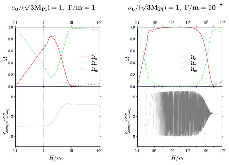
Figure 1: Background energy densities (up) and $\xi_{comp}$ (down) for a large initial value of the field. On the left, a model where the field decays just as it is starting to oscillate and on the right, a model where the field oscillates before decaying. The dotted vertical lines mark the nominal start of oscillation and decay.

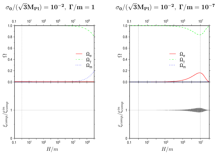
Figure 2: Background energy densities (up) and $\xi_{comp}$ (down) for a small initial value of the field.

The results of the calculation are shown in Figures 1 to 4. In Figures 1 and 2 we show the evolution of the background energy densities and the perturbation variable $\xi_{comp}$. In Figure 1, we have chosen a large initial field value, so the curvaton contributes significantly to the energy density when it decays. On the left, the curvaton has a large decay rate, so that it decays before really starting to oscillate. On the right, the decay rate is small, so that the curvaton oscillates rapidly at the time of decay and thus resembles a pressureless fluid more closely. In Figure 2, we show the analogous plots for a small initial field value, when the curvaton does not contribute significantly to the background before starting to oscillate. Note that even in the model on the left where the curvaton decays before properly oscillating, we recover the dust result $\lambda_{m}=1$.

The surprising result that the dust approximation is valid even when the field does not oscillate when it decays is a general feature, as seen from Figure 3, which shows $\lambda_{m}$ for the whole of our parameter space. The value of $\lambda_{m}$ is practically independent of the decay rate $\Gamma/m$: as long as the initial field value $\sigma_{0}/(\sqrt{3}M_{Pl})$ is less than 0.1 (so that the curvaton does not dominate before oscillating), $\lambda_{m}$ is very close to 1, even when the field decays without any oscillations. On the other hand, for larger values of $\sigma_{0}/(\sqrt{3}M_{Pl})$, $\lambda_{m}$ rises rapidly, up to a maximum of about 350 at the edge of our parameter space.

For fitting our spectrum (26), (27) to the data, we need to know, in addition to $\lambda_{m}$, the ratio $\lambda_{r}/\lambda_{m}$ which measures the relative efficiency of the transfer of the curvaton perturbations to radiation and matter. In Figure 4 we show $\lambda_{r}/\lambda_{m}$ for our parameter space. Like $\lambda_{m}$, the ratio $\lambda_{r}/\lambda_{m}$ is more sensitive to the initial field value $\sigma_{0}/(\sqrt{3}M_{Pl})$ than to the decay rate $\Gamma/m$, though it does grow with decreasing $\Gamma/m$. For small values of the field, the ratio approaches 0 rapidly, and for large values it tends to 1. The upper limit is easy to understand: for large $\sigma_{0}$, the curvaton completely dominates when it decays, so its perturbations are adiabatic, and the perturbations of its decay products have to be adiabatic as well [24], so radiation and matter inherit the same perturbations.

We have studied the validity of the dust approximation, and have surprisingly found that its results for the decay are valid even when the field does not oscillate when it decays. We have also found the range of the parameters $\lambda_{m}$ and $\lambda_{r}/\lambda_{m}$, which we need for fitting our spectrum to CMB data.

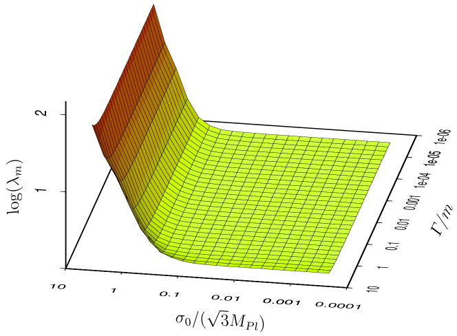
Figure 3: The matter decay coefficient $\lambda_{m}$ on a logarithmic scale.

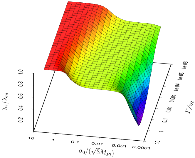
Figure 4: The ratio of the decay coefficients for radiation and matter, $\lambda_{r}/\lambda_{m}$.

3 The fit to WMAP data

3.1 The spectrum of perturbations

Having found the ranges for the parameters for the mixture of inflaton and curvaton perturbations in the spectrum (26), (27), let us now fit the spectrum to the WMAP data and see what such a mixture implies for the CMB anisotropies.

We have not yet specified the inflaton and curvaton spectra $\hat{\mathcal{R}}_{1}$ and $\hat{\mathcal{R}}_{2}$ (in this section we introduce a hat to denote random variable). As the perturbations are assumed to be generated during inflation, the spectra depend on the inflationary model. We will not choose a particular model, but assume that the spectra are given by simple power laws,

$${\textstyle\left(\frac{k^{3}}{2\pi^{2}}\right)^{\frac{1}{2}}}\hat{\mathcal{R}}_{1} = N_{1}\tilde{k}^{\frac{n_{1}-1}{2}}\hat{a}_{1}(\bi{k})$$

$${\textstyle\left(\frac{k^{3}}{2\pi^{2}}\right)^{\frac{1}{2}}}\hat{\mathcal{R}}_{2} = N_{2}\tilde{k}^{\frac{n_{2}-1}{2}}\hat{a}_{2}(\bi{k})\ ,$$ (32)

where $N_{1}$ and $N_{2}$ are constant amplitudes, $n_{1}$ and $n_{2}$ are constant spectral indices and $\tilde{k}=k/k_{0}$ with $k_{0}$ = 0.05 Mpc^-1 is the dimensionless wavenumber. We have denoted by $\hat{a}_{1}(\bi{k})$ and $\hat{a}_{2}(\bi{k})$ Gaussian random variables which obey

$$\langle\hat{a}_{1}\rangle=\langle\hat{a}_{2}\rangle=0\ ,\quad\langle\hat{a}_{i}(\bi{k})\hat{a}_{j}^{*}(\bi{k}^{\prime})\rangle=\delta_{ij}\delta^{(3)}(\bi{k}-\bi{k}^{\prime})\ .$$ (33)

If the perturbation spectra were generated during a period of slow-roll inflation, the spectral indices would be (to first order in the slow-roll parameters) [6, 32]

$$n_{1}=1+2\eta_{1}-6\epsilon_{H}$$

$$n_{2}=1+2\eta_{2}-2\epsilon_{H}\ ,$$ (34)

where $\epsilon_{H}=-\dot{H}/H^{2}$, and $\eta_{1}$ and $\eta_{2}$ are the slow-roll parameters associated with the curvature of the potential in the inflaton and curvaton directions, respectively,

$$\eta_{1} = M_{Pl}^{2}\frac{1}{V}\frac{\partial^{2}V}{\partial\varphi^{2}}$$

$$\eta_{2} = M_{Pl}^{2}\frac{1}{V}\frac{\partial^{2}V}{\partial\sigma^{2}}=\frac{m^{2}}{3H^{2}}\ ,$$ (35)

where $\varphi$ is the inflaton field and $V$ is the inflaton-curvaton-potential $V(\sigma,\varphi)=\frac{1}{2}m^{2}\sigma^{2}+V(\varphi)$ (we neglect inflaton-curvaton interactions). Since the mass of the curvaton is assumed to be much smaller than the Hubble parameter during inflation, $\eta_{2}\ll 1$, and since during slow-roll typically $|\dot{H}|\ll H^{2}$, one might expect $n_{2}$ to be only marginally smaller than 1, though $n_{1}$ could be more different from (and possibly larger than) 1 due to a non-negligible $\eta_{1}$.

However, in the curvaton scenario there is no need to assume that inflation is slow-roll [33] or even that inflationary dynamics are driven by a scalar field [34, 35, 36]. Also, even in single-field inflation the spectral index can be very different from one, while having little running [37, 38, 39]. We do not limit ourselves to slow-roll inflation, and keep the spectral indices as free parameters with a wide range (and do not introduce running for the indices).

In section 2, we calculated the decay of the curvaton into two components, radiation and matter, which inherited the curvaton spectrum with different efficiency coefficients $\lambda_{\alpha}$. In the fit to the CMB, we have four components: baryons, CDM, (massive) neutrinos and photons.

The CDM is assumed to be non-relativistic during the decay, and will therefore inherit the curvaton spectrum with the efficiency $\lambda_{m}$, so its spectrum of perturbations is given by (25). The photons will inherit the curvaton perturbations with the efficiency $\lambda_{r}$, and have the spectrum (24). During curvaton decay, neutrinos are also relativistic, but since the neutrino dilution factor $A_{\nu}$ can be different from the photon dilution factor $A_{\gamma}$, neutrinos and photons could get a different spectrum of perturbations. However, we assume that there is no net lepton number, in which case the neutrinos and photons end up having the same spectrum by virtue of being in thermal equilibrium [10, 40, 41], so there are no neutrino isocurvature perturbations.

Whether the baryons inherit the curvaton spectrum with the efficiency factor for radiation or matter depends on whether the degrees of freedom carrying baryon number are relativistic or non-relativistic during curvaton decay. In any case, there is no reason for the baryon dilution factor $A_{b}$ to be the same as the CDM or photon dilution factors, so there will in general be baryon-CDM and baryon-photon isocurvature perturbations. However, since baryon and CDM isocurvature perturbations behave similarly [13, 40], the isocurvature perturbation between baryons and CDM can be transformed to zero, at the price of adding more isocurvature between CDM and photons. Then the only component with isocurvature perturbations is the CDM, and the spectrum reads

$${\textstyle\left(\frac{k^{3}}{2\pi^{2}}\right)^{\frac{1}{2}}}\hat{\mathcal{R}}^{out}_{\gamma} = (1-A_{\gamma})N_{1}\tilde{k}^{\frac{n_{1}-1}{2}}\hat{a}_{1}(\bi{k})+A_{\gamma}\lambda_{r}N_{2}\tilde{k}^{\frac{n_{2}-1}{2}}\hat{a}_{2}(\bi{k})$$

$${\textstyle\left(\frac{k^{3}}{2\pi^{2}}\right)^{\frac{1}{2}}}\hat{\mathcal{S}}_{cdm,\gamma}^{out} = 3[(A_{cdm}-A_{\gamma})+x_{b}(A_{b}-A_{\gamma})]N_{1}\tilde{k}^{\frac{n_{1}-1}{2}}\hat{a}_{1}(\bi{k})$$ (36)

$$-3[(A_{cdm}\lambda_{m}-A_{\gamma}\lambda_{r})+x_{b}(A_{b}\lambda_{b}-A_{\gamma}\lambda_{r})]N_{2}\tilde{k}^{\frac{n_{2}-1}{2}}\hat{a}_{2}(\bi{k})\ ,$$

where $x_{b}\equiv\rho_{b}/\rho_{cdm}$ and $\lambda_{b}$ is the baryon decay coefficient, which can be either $\lambda_{r}$ or $\lambda_{m}$.

The most general form of a spectrum with an adiabatic plus one isocurvature mode, both of which are a combination of two power laws, has six independent parameters: two spectral indices and four amplitudes (one for each of the two different powers of $\tilde{k}$ for the adiabatic and the isocurvature mode). The expression (3.1) is therefore overdetermined, and though the theoretical interpretation of the parameters is clear, their relation to observable features is murky. We will write the spectrum (3.1) in a form more suited for comparison with observations:

$${\textstyle\left(\frac{k^{3}}{2\pi^{2}}\right)^{\frac{1}{2}}}\hat{\mathcal{R}}^{out}_{\gamma} = N_{\mathcal{R}}\left(\cos\phi\,\tilde{k}^{\frac{n_{1}-1}{2}}\hat{a}_{1}(\bi{k})+\sin\phi\,\tilde{k}^{\frac{n_{2}-1}{2}}\hat{a}_{2}(\bi{k})\right)$$

$${\textstyle\left(\frac{k^{3}}{2\pi^{2}}\right)^{\frac{1}{2}}}\hat{\mathcal{S}}_{cdm,\gamma}^{out} = N_{\mathcal{R}}f_{\mathcal{S}}\left(\cos\theta\,\tilde{k}^{\frac{n_{1}-1}{2}}\hat{a}_{1}(\bi{k})-\sin\theta\,\tilde{k}^{\frac{n_{2}-1}{2}}\hat{a}_{2}(\bi{k})\right)\ ,$$ (37)

where the new constant parameters $N_{\mathcal{R}},f_{\mathcal{S}},\phi,\theta$ can be written in terms of the old parameters in (3.1) (the inverse is obviously not true, since (3.1) has more parameters than (3.1)).

The new parameters have a transparent interpretation in terms of observable quantities: $N_{\mathcal{R}}$ is the amplitude of the adiabatic perturbations, the isocurvature fraction $f_{\mathcal{S}}$ measures the amplitude of the isocurvature perturbations relative to the adiabatic ones, and the angles $\phi$ and $\theta$ determine the proportion of the adiabatic and isocurvature perturbations, respectively, that have the spectral index $n_{1}$ or $n_{2}$.

The generality of the spectrum (3.1) goes beyond the inflaton-curvaton model that we have discussed. It is the most general form for the case when baryons, CDM and photons inherit power-law perturbations from two independent sources. For example, it could describe a double inflation model. Also, in realistic supersymmetric GUT theories, cosmic strings are typically produced after inflation, leading to isocurvature perturbations [43]. The isocurvature perturbations produced by cosmic strings are usually considered to be uncorrelated with the pre-existing adiabatic perturbations from the inflationary era, but if they were correlated and the strings would decay, a spectrum like (3.1) might result.

In the general case, the ranges for the parameters in (3.1) are as follows. The amplitude $N_{\mathcal{R}}$ is positive, the isocurvature fraction $f_{\mathcal{S}}$ can be negative, positive or zero, the angle $\phi$ is from the interval $[0,\pi/2]$ and the angle $\theta$ is from the interval $[0,\pi]$.

Note that the roles of the inflaton and the curvaton are completely symmetric: the spectrum (3.1) is invariant under the transformation $n_{1}\leftrightarrow n_{2}$, $\cos\phi\leftrightarrow\sin\phi$, $\cos\theta\leftrightarrow\mbox{sign}(\cos\theta)\sin\theta$ and $f_{S}\rightarrow-\mbox{sign}(\cos\theta)f_{S}$. To avoid scanning the parameter space twice, we break the symmetry by writing $n_{1}=n_{2}+\Delta n$ and studying only models where the inflaton spectral index is larger than or equal to the curvaton spectral index, $\Delta n\geq 0$.

If the transfer of curvaton perturbations to matter and radiation were equally efficient, $\lambda_{r}=\lambda_{m}$, then $\sin\theta$ and $\cos\theta$ would necessarily have the same sign, so that $\theta$ would be restricted to the range $[0,\pi/2]$. In our model the transfer to matter is more efficient than the transfer to radiation, $\lambda_{r}<\lambda_{m}$, so that $\theta$ has the full range $[0,\pi]$ when $f_{\mathcal{S}}>0$, but is restricted to the range $[0,\pi/2]$ when $f_{\mathcal{S}}<0$. So, the role of the decay coefficients $\lambda_{\alpha}$ is to expand the range of $\theta$ in the spectrum (3.1). In our analysis we will allow $\theta$ to vary between $[0,\pi]$, and at the end remove the forbidden region $f_{\mathcal{S}}<0,\theta>\pi/2$.

3.2 Angular power and (anti)correlation

The angular power spectra.

The temperature-temperature (TT) angular power spectrum resulting from the primordial spectra (3.1) is

$$C_{l}^{TT} = 4\pi\int\frac{\rmd k}{k}\frac{k^{3}}{2\pi^{2}}\langle|g_{l,\mathcal{R}}^{T}(k)\hat{\mathcal{R}}(\bi{k})+g_{l,\mathcal{S}}^{T}(k)\hat{\mathcal{S}}(\bi{k})|^{2}\rangle$$ (39)

$$= 4\pi\int\frac{\rmd k}{k}\frac{k^{3}}{2\pi^{2}}\left(g_{l,\mathcal{R}}^{T}(k)^{2}\langle|\hat{\mathcal{R}}(\bi{k})|^{2}\rangle+g_{l,\mathcal{S}}^{T}(k)^{2}\langle|\hat{\mathcal{S}}(\bi{k})|^{2}\rangle\right.$$

$$\left.+g_{l,\mathcal{R}}^{T}(k)g_{l,\mathcal{S}}^{T}(k)\langle\hat{\mathcal{R}}(\bi{k})\hat{\mathcal{S}}(\bi{k})^{*}+\hat{\mathcal{R}}(\bi{k})^{*}\hat{\mathcal{S}}(\bi{k})\rangle\right)$$

$$= 4\pi\int\frac{\rmd k}{k}N_{\mathcal{R}}^{2}\left[g_{l,\mathcal{R}}^{T}(k)^{2}\left(\cos^{2}\phi\,\tilde{k}^{n_{1}-1}+\sin^{2}\phi\,\tilde{k}^{n_{2}-1}\right)\right.$$

$$+f_{\mathcal{S}}^{2}\,g_{l,\mathcal{S}}^{T}(k)^{2}\left(\cos^{2}\theta\,\tilde{k}^{n_{1}-1}+\sin^{2}\theta\,\tilde{k}^{n_{2}-1}\right)$$

$$\left.+2g_{l,\mathcal{R}}^{T}(k)f_{\mathcal{S}}g_{l,\mathcal{S}}^{T}(k)\left(\cos\phi\cos\theta\,\tilde{k}^{n_{1}-1}-\sin\phi\sin\theta\,\tilde{k}^{n_{2}-1}\right)\right]$$

$$= 4\pi\int\frac{\rmd k}{k}N_{\mathcal{R}}^{2}\left[\left(g_{l,\mathcal{R}}^{T}(k)\cos\phi+f_{\mathcal{S}}g_{l,\mathcal{S}}^{T}(k)\cos\theta\right)^{2}\tilde{k}^{n_{1}-1}\right.$$

$$\left.+\left(g_{l,\mathcal{R}}^{T}(k)\sin\phi-f_{\mathcal{S}}g_{l,\mathcal{S}}^{T}(k)\sin\theta\right)^{2}\tilde{k}^{n_{2}-1}\right]\ ,$$

where $g_{l,\mathcal{R}}^{T}(k)$ and $g_{l,\mathcal{S}}^{T}(k)$ are the functions which transfer the primordial curvature and entropy perturbations of the mode with the wavenumber $k$ from the early radiation-dominated era to the present temperature fluctuation at the multipole $l$. Written like this, the role of $f_{\mathcal{S}}$ in scaling the amplitude of the isocurvature modes via $g_{l,\mathcal{S}}^{T}(k)$ is particularly transparent.

For the temperature-polarisation (TE) cross-correlation power spectrum we have

$$C_{l}^{TE}=4\pi\int\frac{\rmd k}{k}\frac{k^{3}}{2\pi^{2}}\langle[g_{l,\mathcal{R}}^{T}(k)\hat{\mathcal{R}}(\bi{k})+g_{l,\mathcal{S}}^{T}(k)\hat{\mathcal{S}}(\bi{k})]^{*}\times[g_{l,\mathcal{R}}^{E}(k)\hat{\mathcal{R}}(\bi{k})+g_{l,\mathcal{S}}^{E}(k)\hat{\mathcal{S}}(\bi{k})]\rangle\ ,$$ (40)

where $g_{l,\mathcal{R}}^{E}(k)$ and $g_{l,\mathcal{S}}^{E}(k)$ are the transfer functions for the polarisation $E$-mode (for details see e.g. [44]).

There are six different terms in (39). The first two are due to the primordial adiabatic perturbations $\hat{\mathcal{R}}^{out}_{\gamma}$, and they will be denoted by $C_{l}^{\rm adi1}$ and $C_{l}^{\rm adi2}$. The next two terms are due to the primordial isocurvature perturbations $\hat{\mathcal{S}}^{out}_{cdm,\gamma}$, and they will be denoted by $C_{l}^{\rm iso1}$ and $C_{l}^{\rm iso2}$. Finally, the last two terms arise from the correlation between adiabatic and isocurvature perturbations, and will be denoted by $C_{l}^{\rm cor1}$ and $C_{l}^{\rm cor2}$. The same notation will be used for the components of the TE power spectrum.

The role of CDM isocurvature perturbations.

The acoustic peak structure in the measured angular power spectrum looks distinctly adiabatic. CDM isocurvature perturbations have valleys where adiabatic perturbations have peaks and are also damped faster with increasing $l$. Therefore pure CDM isocurvature perturbations cannot fit the data and are ruled out [45]. However, a mixture where adiabatic perturbations dominate the peak structure and CDM isocurvature perturbations give a significant contribution at low multipoles remains an interesting possibility.

At low multipoles the Sachs-Wolfe effect gives $g_{l,\mathcal{S}}^{T}(k)=-2(1-f_{\nu})g_{l,\mathcal{R}}^{T}(k)$. The rapid damping of $g_{l,\mathcal{S}}^{T}(k)$ with increasing $l$ means that if the primordial adiabatic and isocurvature perturbation amplitudes are of the same order, the isocurvature perturbations modify only the low-$l$ part (practically the Sachs-Wolfe plateau) of the final $C_{l}$ spectrum observed today. This is natural in our model where baryons, CDM and photons are all generated by both inflaton and curvaton decay. In terms of the spectrum (3.1), this means $f_{\mathcal{S}}\sim 1$, which is the generic value. To get a much larger or smaller value, one has to tune the model in some way (say, by having $A_{\gamma}=A_{cdm}=A_{b}$ to a high accuracy).

Uncorrelated adiabatic and isocurvature perturbations add power on the SW plateau relative to the acoustic peaks, and since the observations indicate a deficit of power, this does not improve the fit to the data [46]. However, in our model the adiabatic and isocurvature perturbations are correlated. Negative correlation will naturally suppress the power on the SW plateau and thus improve the fit. The suppression is large if $\hat{\mathcal{R}}\sim\hat{\mathcal{S}}$, and total when $\hat{\mathcal{R}}=2(1-f_{\nu})\hat{\mathcal{S}}$. Again, note that our model naturally yields $\hat{\mathcal{R}}\sim\hat{\mathcal{S}}$ which is required for significant cancellation. Also, as we will discuss in section 3.6, our spectrum (3.1) gives more freedom to adjust the cancellation of the low multipoles than in previous studies of suppression due to anticorrelation [7, 9, 21, 44, 47, 48, 49, 50, 51, 52].

We note in passing that the conclusion that the peak structure excludes a sizeable contribution from CDM isocurvature modes outside of the SW plateau does not hold for neutrino density and neutrino velocity isocurvature modes, since their peak structure is similar to that of adiabatic modes [40, 53]. In fact, there is an explicit example where isocurvature modes give a major contribution to all of the observed acoustic peaks [54].

3.3 Fitting method

We fit the spectra (39) and (40) to the WMAP first-year data [55, 56, 57] by running several Monte Carlo chains on a supercomputer. We vary the following 11 primary parameters (parameter ranges are given in Table 1). We have five standard parameters related to the cosmological background, called the hard parameters: the physical baryon density $\omega_{b}=h^{2}\Omega_{b}$, the physical dark matter density $\omega_{dm}=h^{2}\Omega_{dm}$, the ratio of the sound horizon to the angular diameter distance (i.e. the acoustic peak scale in radians) $\Theta$, the optical depth due to reionisation $\tau$ and the neutrino fraction $f_{\nu}=\omega_{\nu}/\omega_{dm}$. We also assume that there is vacuum energy, the density of which is fixed by the constraint that the universe is spatially flat, $\Omega_{\Lambda}+\Omega_{m}=1$, where $\Omega_{m}=\Omega_{b}+\Omega_{dm}$. We have six parameters for the spectrum of perturbations, instead of the usual two: the spectral index $n_{1}$, the difference between the spectral indices $\Delta n=n_{1}-n_{2}$, the overall normalisation $\ln(10^{10}N_{\mathcal{R}}^{2})$, the fraction of adiabatic perturbations that come from the inflaton $\cos\phi$, the fraction of isocurvature perturbations that come from the inflaton $\cos\theta$, and the CDM-photon isocurvature fraction $f_{\mathcal{S}}$.

The technical details of our analysis are very similar to those described in the appendix of [58]. We use a modified version of CosmoMC [59] to generate 40 Monte Carlo Markov Chains that start from randomly chosen points in the parameter space. The transfer functions $g_{l,\mathcal{R}}^{T}(k)$, $g_{l,\mathcal{S}}^{T}(k)$, $g_{l,\mathcal{R}}^{E}(k)$, and $g_{l,\mathcal{S}}^{E}(k)$ are calculated with our modified version of CAMB [60] whenever any hard parameter is changed. The integrals (39) and (40) are then evaluated for each model. After running between 8 and 12 days, each chain contains about 10 000 accepted steps (150 000 step trials). We cut off burn-in periods and neglect 13 chains that never burned-in but instead got stuck in a local likelihood minimum. The correlation length (i.e. the number of steps between independent samples) is quite long in our chains, typically 170 – 1000. Nevertheless, after the described procedure, we still have over 220 000 accepted steps (3 300 000 step trials) giving 7500 independent samples to analyse.

In the same way, we create chains for a $\Lambda$CDM model with adiabatic power-law perturbations (and without massive neutrinos) to serve as a reference point. The 6 primary parameters of the reference model are $\omega_{b}$, $\omega_{dm}$, $\Theta$ and $\tau$ for the background and $n$, $\ln(10^{10}N_{\mathcal{R}}^{2})$ for the perturbations.

We produce a 1-dimensional marginalised likelihood distribution (probability density) for each primary parameter and for some derived parameters such as the spectral index $n_{2}$, the dark matter-photon isocurvature fraction $\tilde{f}_{\mathcal{S}}$, the vacuum energy density $\Omega_{\Lambda}$, the baryon energy density $\Omega_{b}$, the matter energy density $\Omega_{m}$, the CDM energy density $\Omega_{cdm}$, the (massive) neutrino energy density $\Omega_{\nu}$, the age of the universe, the reionisation redshift $z_{re}$ and the Hubble parameter today $H_{0}=h\times 100$ km/s/Mpc.

We do not apply any priors to primary parameters, but use a top-hat prior $0.21<h<1.00$ for the Hubble parameter and $\Omega_{\Lambda}\geq 0$ for the vacuum energy density. The main focus of the present paper is the study of the perturbation spectrum in the mixed inflaton-curvaton model, so we will here simply do a fit to the WMAP data, and briefly discuss the interesting features of the fit. We will follow up with a more detailed analysis of cosmological parameter evaluation in a separate paper [23], where we will also include data from high-$l$ CMB measurements and the Sloan Digital Sky Survey (SDSS) [58, 61].

3.4 Results of the data fit

There are 1348 WMAP data points and our model has 11 parameters, so the reduced number of degrees of freedom is $\nu=1348-11=1337$. The reference pure adiabatic $\Lambda$CDM model has 6 parameters giving $\nu=1342$. Our best-fit model has $\chi^{2}=1423.9$ and the best-fit reference model has $\chi^{2}=1429.0$. In the first two columns of Table 1 we compare the parameters of these models. Even though our model has a better $\chi^{2}$ value, $\chi^{2}/\nu$ turns out to be exactly the same (1.065) for both models. Thus this measure-of-goodness does not support introducing the isocurvature degrees of freedom. However, we are interested in the SW plateau (in particular the quadrupole power) beyond its statistical weight in the overall fit. On the last three lines of Table 1 we give the quadrupole power of both models as well as the $\chi^{2}$ of the first two data points (quadrupole and octopole) and their contribution to the total $\chi^{2}$. The quadrupole power in our best-fit model is 125 $\mu$K² smaller than in the $\Lambda$CDM model. This makes our fit better in the SW plateau and drops the $\chi^{2}$ contribution of the first two data points from 0.51% to 0.45%.

The parameters of the best-fit model are somewhat exotic. The physical baryon density $\omega_{b}=0.041$ is much larger than the value given by BBN [63]. The large neutrino density $f_{\nu}=0.86$ implies (along with $\omega_{dm}=0.12$) that the sum of neutrino masses is 9.2 eV, in conflict with measurements of tritium decay which give an upper limit of $m_{\nu_{e}}=2.2$ eV for the electron neutrino mass [64], yielding an upper limit of 6.6 eV for the sum of neutrino masses (when combined with the small mass differences from oscillation experiments). Note also the very small CDM density, $\Omega_{cdm}=0.028$. One would expect this to be highly problematic for structure formation, but on the other hand the spectral index on the relevant scales is deeply blue, $n_{1}=3.9$, which significantly enhances the amplitude of perturbations on the scales probed by the measurements of large-scale structure.

The best-fit isocurvature model (for which we do not give a $C_{l}$ plot) is not meant to be taken as an alternative to the best-fit adiabatic power-law $\Lambda$CDM model. Rather, it underlines the point that models with radically different background cosmologies and perturbation spectra can fit the WMAP data even slightly better than the standard model. Including CDM isocurvature perturbations opens up the space of well-fitting models, and the cosmological parameters in these models are no longer clustered around the best-fitting model. The addition of priors from other cosmological observations, as well as data on the power spectrum from high-$l$ CMB measurements and large-scale structure will exclude many of these models. For example, our best-fit model does not fit the data from high-$l$ CMB measurements: the nearly scale-free spectral index $n_{2}=0.988$ dominates until the third acoustic peak, but the large spectral index $n_{1}=3.906$ gives too much power in the region $l>900$.

For now, the message to take away is that one cannot determine the cosmological parameters from the WMAP data alone with any degree of confidence without making strong assumptions about the primordial power spectrum. Turning this around, it is not possible to determine the primordial power spectrum using only the WMAP data without making strong assumptions about the cosmological parameters. This has been previously emphasised in [65, 66]. As a warning example, we note that the original implementation of the pre-big bang scenario [67] was ruled out in part because the spectral index $n=4$ of the adiabatic perturbations coming from the dilaton was too large to fit the CMB data, and the second version [68] was ruled out because the axion with a spectral index $n=1$ carried only isocurvature perturbations. Implementing the pre-big bang curvaton model for the axion [5, 11], but keeping the dilaton perturbations would lead to our spectrum (3.1) with the spectral indices $n_{1}=4$ and $n_{2}=1$, which incidentally agree with our best-fit model.

	Adiabatic	Our	Our	Adiabatic	Our model
	best-fit	best-fit	example
$\chi^{2}$	1429.0	1423.9	1425.9
$\nu$	1342	1337	1337
$\chi^{2}/\nu$	1.065	1.065	1.066
Primary parameters
$\omega_{b}$ [0.005, 0.1]	0.0229	0.0409	0.0284	${0.0238}_{-0.0015}^{+0.0026}$	${0.0315}_{-0.0044}^{+0.0107}$
$\omega_{dm}$ [0.01, 0.99]	0.122	0.115	0.150	${0.118}_{-0.018}^{+0.018}$	${0.125}_{-0.024}^{+0.023}$
$100\times\Theta$ [0.3, 10]	1.044	1.074	1.060	${1.049}_{-0.007}^{+0.008}$	${1.062}_{-0.013}^{+0.016}$
$\tau$ [0.01, 0.8]	0.115	0.498	0.127	${0.159}_{-0.074}^{+0.157}$	${0.222}_{-0.114}^{+0.227}$
$f_{\nu}$ [0, 1]	—	0.855	0.725	—	$>$ 0.8
$n_{1}$ [0.2, 4]	0.964	3.906	1.065	${0.992}_{-0.037}^{+0.083}$	${1.377}_{-0.289}^{+1.600}$
$\Delta n$ [0, 3.8]	—	2.918	0.220	—	($<$ 1.06)
$\ln(10^{10}N_{\mathcal{R}}^{2})$ [1, 6]	3.950	4.492	3.884	${4.054}_{-0.166}^{+0.310}$	${4.031}_{-0.242}^{+0.413}$
$\cos\phi$ [0, 1]	(1)	0.295	0.422	(1)	no constraint
$\cos\theta$ [-1, 1]	—	0.985	0.731	—	$>$ 0.76
$f_{\mathcal{S}}$ [-42, 42]	(0)	-9.156	-1.400	(0)	$|f_{\mathcal{S}}|<$ 13
Derived parameters
$n_{2}$	—	0.988	0.845	—	${0.869}_{-0.160}^{+0.205}$
$\tilde{f}_{\mathcal{S}}=(1-f_{\nu})f_{\mathcal{S}}$	(0)	-1.329	-0.385	(0)	$|\tilde{f}_{\mathcal{S}}|<$ 0.7
$\Omega_{\Lambda}$	0.695	0.736	0.345	${0.726}_{-0.084}^{+0.087}$	${0.627}_{-0.243}^{+0.141}$
$\Omega_{b}$	0.048	0.069	0.103	${0.046}_{-0.008}^{+0.008}$	${0.079}_{-0.019}^{+0.025}$
$\Omega_{m}$	0.305	0.264	0.655	${0.274}_{-0.087}^{+0.084}$	${0.373}_{-0.141}^{+0.244}$
$\Omega_{cdm}$	0.257	0.028	0.151	${0.229}_{-0.079}^{+0.076}$	$<$ 0.06
$\Omega_{\nu}$	—	0.166	0.399	—	${0.239}_{-0.124}^{+0.213}$
Age (Gyr)	13.62	12.68	14.32	${13.39}_{-0.51}^{+0.30}$	${13.69}_{-1.16}^{+0.95}$
$z_{re}$	13.73	25.93	13.45	${16.86}_{-5.73}^{+7.78}$	${18.41}_{-7.78}^{+7.87}$
$H_{0}$ (km/s/Mpc)	68.87	77.02	52.21	${71.78}_{-5.36}^{+10.10}$	${64.29}_{-11.38}^{+15.87}$
Low-$l$ behaviour
$2(2+1)C_{2}/2\pi$ ($\mu$K2)	1170	1045	736	(mean) ${1262}_{-190}^{+202}$	(mean) ${1081}_{-226}^{+225}$
$\chi^{2}(C_{2},C_{3})$	7.338	6.408	4.336	(mean) 7.888	(mean) 6.615
$\chi^{2}(C_{2},C_{3})/\chi^{2}$ (%)	0.514	0.450	0.304	(mean) 0.550	(mean) 0.461

Table 1: Comparison of models. In the last two columns we give the median of the 1-dimensional marginalised likelihood for each parameter and the region around the median that contains 68% of the accepted models in our chains. If the likelihood function was exactly Gaussian, this would correspond to the $1\sigma$ region. However, most of the likelihood functions are too far from Gaussian for this to be true, as should be clear from the values of our best-fit model. Thus the parameter ranges should not be taken as $1\sigma$ regions. They are given for comparison purposes only.

3.5 Likelihood distributions

Let us briefly discuss the main features of the marginalised likelihood distributions, concentrating on the differences between our isocurvature model and the pure adiabatic $\Lambda$CDM model.

In Table 1 we give the median values for the primary and derived parameters, and the regions that contain 68% of the accepted models in the 1-dimensional marginalised likelihood distributions for the adiabatic model and for our model. As the likelihood function is non-Gaussian with respect to some parameters, most of the quoted numbers cannot be interpreted as 1$\sigma$ confidence levels and are for comparison purposes only. (The meaning of the given values is as described in the appendix of [58].) Of the primary and derived parameters, only $\omega_{dm}$, $\Theta$, $n_{2}$, $\Omega_{cdm}$ and the age of the universe have a strongly Gaussian 1-d marginalised likelihood distribution. Of course, even for these parameters, the numbers are confidence ranges, and should not be treated as exclusion limits, as emphasised in [66]. Adding more input into our analysis, such as the SDSS data [58, 61] would lead to better behaved likelihood distributions, in agreement with the discussion above.

The well-known degeneracy between the physical baryon density $\omega_{b}$ and isocurvature modes [44, 54, 65] is apparent also from our results. In a pure adiabatic power-law model, $\omega_{b}$ is determined simply by the relative heights of the successive acoustic peaks. Since the CDM isocurvature mode has valleys where the adiabatic mode has peaks, increasing the relative isocurvature contribution can compensate for adding baryons. This, and the fact that the modes are the sum of two power-laws, means that there is much more freedom for the values of $\omega_{b}$ in our model than in a pure adiabatic model. Also, the preferred values of $\omega_{b}$ with isocurvature modes are generally higher than in the pure adiabatic case.

The optical depth $\tau$ is poorly constrained in the pure adiabatic case, and even more so in our model. The 95% region spans a huge range from 0.05 to 0.59, and the 68% region given in Table 1 is also wide. The optical depth is primarily determined by the single data point at $l=2$ in the WMAP TE data. This quadrupole TE power is very high, hinting at early reionisation (large optical depth) in the pure adiabatic case. In our model the mechanism that suppresses the low TT multipoles also cancels TE power, which means that an even larger $\tau$ is needed to fit the high first data point; on the other hand, positive correlation would add TE power at the quadrupole and allow a smaller $\tau$. Note that in the pure adiabatic case, the signal for the large optical depth in the TT spectrum comes completely from the southern hemisphere; the preferred value for the northern hemisphere is $\tau=0$ [69]. Such asymmetry suggests caution about the interpretation of the data points leading to the value of $\tau$. At any rate, the effect on our results is small, since they are consistent with a wide range of values.

In the pure adiabatic power-law model there is only one spectral index while our model has two, so a simple comparison of their values is not very meaningful. However, let us mention that while the peak of the likelihood function for the larger spectral index $n_{1}$ is at the moderate value 1.1, the distribution has a long tail at large values, so that the median is 1.4 and the mean is even larger, 1.8. While this may be an artifact of poor convergence of $\Delta n$ (the split test shows that the upper bound for $\Delta n$ is not reliable), our best-fit model with $n_{1}=3.9$ demonstrates that the WMAP data does not require the spectrum to be almost scale-invariant over the entire range of scales covered by the data.

The vacuum energy density $\Omega_{\Lambda}$ is much less constrained than in pure adiabatic models. The reason is again low-$l$ modifications. Increasing $\Omega_{\Lambda}$ raises the TT power at the lowest multipoles due to the integrated Sachs-Wolfe effect. This effect can be countered by negative correlation which brings the low multipoles down, or mimicked by positive correlation which takes them up. The net effect is to widen the range of $\Omega_{\Lambda}$ in both directions. The Hubble parameter and vacuum energy density are strongly correlated, so the freedom in the values of $\Omega_{\Lambda}$ is reflected in the values of $H_{0}$.

It is notable that our isocurvature spectrum prefers a large neutrino fraction $f_{\nu}$, in contrast to a pure adiabatic spectrum which is not very sensitive to the value of $f_{\nu}$ [58, 70, 71, 72]. Our model differentiates between CDM and massive neutrinos because the latter carry no isocurvature perturbations. This means that for fixed dark matter density and CDM isocurvature amplitude, one can tune down the isocurvature contribution by increasing the neutrino fraction $f_{\nu}$: the less CDM there is, the less difference its perturbations make. The total dark matter-photon isocurvature perturbation $\mathcal{S}_{dm,\gamma}$ and cold dark matter-photon isocurvature perturbation $\mathcal{S}_{cdm,\gamma}$ are related by $\mathcal{S}_{dm,\gamma}=(1-f_{\nu})\mathcal{S}_{cdm,\gamma}$, so the power spectrum is almost (but not entirely) degenerate with respect to scaling $f_{\mathcal{S}}$ and $1/(1-f_{\nu})$ by the same factor. As it is, our model seems to prefer a high CDM-photon isocurvature fraction $f_{\mathcal{S}}$, with a large neutrino fraction to compensate. A meaningful measure of the isocurvature contribution is given by the dark matter-photon isocurvature fraction $\tilde{f}_{\mathcal{S}}=(1-f_{\nu})f_{\mathcal{S}}$. We find $|\tilde{f}_{\mathcal{S}}|<0.7$ in the 68% region (in agreement with [44, 49, 73]), though a look at our best-fit model with $\tilde{f}_{\mathcal{S}}=-1.3$ should again serve as a warning not to interpret this number as an exclusion limit.

Since $f_{\mathcal{S}}$ and $1-f_{\nu}$ are almost degenerate, measuring one will constrain the other. As CDM and neutrinos have a very different effect on the matter power spectrum [58, 70], using the SDSS data to give a handle on the neutrino fraction could indirectly constrain the isocurvature contribution (which is itself negligible at the SDSS scales since the isocurvature perturbations are damped rapidly with increasing $l$).

Finally, from Table 1 we see that the mean TT quadrupole power in the MC chains for our model is 181 $\mu$K² smaller than for pure adiabatic models. This shows that the cancellation mechanism works and on average helps in fitting the low-$l$ part of the spectrum. The mean $\chi^{2}$ contribution of the first two TT data points to the total $\chi^{2}$ is also reduced from 0.55% to 0.46%. We devote the next section to this important issue.

3.6 Suppression of the low multipoles

The most important feature of the angular power spectrum that distinguishes the inflaton-curvaton model from the standard adiabatic power-law $\Lambda$CDM model is the amplitude of the low multipoles. In fact, this is the only significant qualitative difference, which is not surprising. As discussed in section 3.2, the pure adiabatic $\Lambda$CDM model fits the TT power spectrum very well, apart from the low multipoles and the three “blips” at intermediate multipoles before and at the first acoustic peak (see Figure 6). The three blips cannot be fitted with the smooth CDM isocurvature modes, so the only place where we can get significant improvement is the low multipoles.

While the discrepancy of the low multipoles in the adiabatic $\Lambda$CDM model looks significant to the eye (see Figure 6), the small number of badly fitted data points (practically the first two points) combined with the large cosmic variance means that the weight of this feature in the overall $\chi^{2}$ fit is quite small (for the best-fit adiabatic model only 0.51%, or 7 points, of the total $\chi^{2}$). Therefore one does not expect any model that does not explain the “blips” to have a significantly lower $\chi^{2}$ than the pure adiabatic $\Lambda$CDM case, regardless of what the model is. Indeed, the difference in $\chi^{2}$ between the best-fit pure adiabatic model and the best-fit inflaton-curvaton model is only 5: our model fits better, but not decisively better.

However, the small amplitude of the low multipoles is an interesting feature beyond its statistical significance, and has attracted a lot of attention. Since a $\chi^{2}$-selection among models does not particularly pick out ones with small amplitude for the low multipoles (in our best-fit model, less than 1 point of the improvement in the $\chi^{2}$ comes from the quadrupole and octopole), we specifically look for low quadrupole power among those of our models that fit the data nearly as well as the best-fit model. (The inclusion of data from high-$l$ CMB measurements and SDSS would further reduce the weight of the low multipoles in the overall fit, making it more difficult to find models with a low quadrupole.)

We take a model found using this method as our example with which to demonstrate the suppression mechanism of the low multipoles. The parameters for the example model are given in the third column of Table 1. The TT and TE angular power spectra of the example model and the contributions from the individual adiabatic, isocurvature and correlation components are shown in Figure 5. In Figure 6 the inflaton and curvaton contributions and the total TT spectrum are plotted in comparison to the adiabatic power-law $\Lambda$CDM model.

The example model has $\chi^{2}=1425.9$, which is 2 larger than our best-fit, and still 3 smaller than the adiabatic best-fit. On the last three lines of Table 1 we compare the best-fit adiabatic $\Lambda$CDM model, our best-fit model and our example model. We give the quadrupole power, the $\chi^{2}$ of the first two data points (quadrupole and octopole) and their contribution to the total $\chi^{2}$. The quadrupole power in our example model is 736 $\mu$K², which is 434 $\mu$K² smaller than in the best-fit adiabatic model. This makes the fit better on the SW plateau and drops the $\chi^{2}$ contribution of the first two data points from 0.51% to 0.30%. Note that unlike in our best-fit model, practically all of the improvement in the $\chi^{2}$ over the adiabatic case comes from the low multipoles.

For comparison purposes, we also did a search for low quadrupole power among $\Lambda$CDM models that are within $\Delta\chi^{2}<2$ from the best-fit $\Lambda$CDM model. As expected, the lowest quadrupole power found (914 $\mu$K²) is significantly higher than in our example model.

   

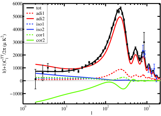
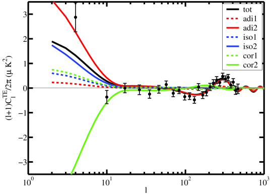
Figure 5: The example model of the third column of Table 1 with the WMAP data ($\bullet$) and the highest $l$ data points of other CMB experiments from Tegmark’s compilation [70] ($\blacklozenge$). The total angular power consists of the six components mentioned in the paragraph after equation (40): $C_{l}^{\rm tot}=C_{l}^{\rm adi1}+C_{l}^{\rm iso1}+C_{l}^{\rm cor1}+C_{l}^{\rm adi2}+C_{l}^{\rm iso2}+C_{l}^{\rm cor2}$. Upper panel: Temperature-temperature angular power $l(l+1)C_{l}^{TT}/2\pi$. Lower panel: Temperature-polarisation cross-correlation power $(l+1)C_{l}^{TE}/2\pi$.

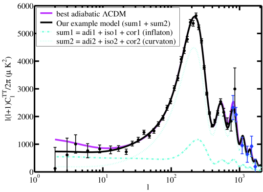
Figure 6: Comparison of our example model (the third column of Table 1, see also Figure 5) to the best-fit 6-parameter adiabatic $\Lambda$CDM model (the first column of Table 1). The total angular power of our model is the black solid line; $C_{l}^{\rm tot}=C_{l}^{\rm sum1}+C_{l}^{\rm sum2}$, where $C_{l}^{\rm sum1}=C_{l}^{\rm adi1}+C_{l}^{\rm iso1}+C_{l}^{\rm cor1}$ and $C_{l}^{\rm sum2}=C_{l}^{\rm adi2}+C_{l}^{\rm iso2}+C_{l}^{\rm cor2}$.

Extreme cancellation.

Let us look at the details of the suppression mechanism of the low multipoles with the spectrum (3.1). If we wanted to pull the amplitude on the SW plateau down as much as possible, we could put $\cos\phi=0$ in (39) to kill $C_{l}^{\rm adi1}$ and $C_{l}^{\rm cor1}$, and then use anticorrelation to get rid of $C_{l}^{\rm adi2}+C_{l}^{\rm iso2}+C_{l}^{\rm cor2}$ on the SW plateau. Given that $g_{l,\mathcal{S}}^{T}(k)=-2(1-f_{\nu})g_{l,\mathcal{R}}^{T}(k)$ on the SW plateau, this implies, from (39), that $\sin\phi+2(1-f_{\nu})f_{\mathcal{S}}\sin\theta=0$. The TT spectrum would then be

$$C_{l}^{TT}=4\pi\int\frac{\rmd k}{k}N_{\mathcal{R}}^{2}\left[\left(\frac{g_{l,\mathcal{S}}^{T}(k)}{2(1-f_{\nu})}\right)^{2}\cot^{2}\theta\,\tilde{k}^{n_{1}-1}+\left(g_{l,\mathcal{R}}^{T}(k)+\frac{g_{l,\mathcal{S}}^{T}(k)}{2(1-f_{\nu})}\right)^{2}\tilde{k}^{n_{2}-1}\right]\ ,$$ (41)

and we have $\cos\phi=0$, $\tilde{f}_{\mathcal{S}}=-1/(2\sin\theta)$. On the SW plateau, the second term is zero, and the spectrum has the index $n_{1}$, with an amplitude that is freely adjustable with $\cot^{2}\theta$. Away from the plateau, the isocurvature transfer function $g_{l,\mathcal{S}}^{T}(k)$ is damped more rapidly than the adiabatic transfer function $g_{l,\mathcal{R}}^{T}(k)$, so the spectrum at high multipoles is essentially adiabatic, has the spectral index $n_{2}$ and an amplitude given by $N_{\mathcal{R}}^{2}$. Since we have $n_{1}>n_{2}$, the low multipoles are further suppressed relative to the high multipoles.

In other words, the low multipoles are given by inflaton isocurvature perturbations with the larger spectral index $n_{1}$, while the peak structure is given by adiabatic curvaton perturbations with the smaller spectral index $n_{2}$. The SW plateau and the peak structure can therefore be adjusted almost independently to fit the data.

Cancellation in our example model.

In contrast to the extreme case, in our example model the behaviour of the high multipoles is not completely decoupled from that of the low multipoles. However, the cancellation mechanism for the low multipoles works qualitatively as sketched above: a small $\cos\phi$ suppresses the adiabatic and correlation components $C_{l}^{\rm adi1}$ and $C_{l}^{\rm cor1}$ with the larger spectral index $n_{1}$, and strong anticorrelation suppresses all three components $C_{l}^{\rm adi2}$, $C_{l}^{\rm iso2}$ and $C_{l}^{\rm cor2}$ with the smaller spectral index $n_{2}$.

From Figures 5 and 6 we see that the curvaton perturbations with the spectral index $n_{2}=0.85$ are killed almost completely by the anticorrelation at the low multipoles, but they dominate the peak structure. The power at low multipoles comes almost completely from the inflaton perturbations, with $n_{1}=1.07$. However, in contrast to the extreme case, the amplitude of the adiabatic component $C_{l}^{\rm adi1}$ is not exactly zero, and it gives a significant subdominant contribution to the acoustic peaks. For the first peak, the inflaton and curvaton correlation modes $C_{l}^{\rm cor1}$ and $C_{l}^{\rm cor2}$ also contribute. The correlation results in peak structure between pure adiabatic and pure isocurvature cases, and the fact that those components are themselves a sum of two power-laws also slightly modifies the relative heights of the successive peaks (and valleys).

Since our example model has a non-zero vacuum energy density ($\Omega_{\Lambda}=0.35$), the integrated SW effect would typically lead to rising power towards the smallest multipoles (as apparent for the adiabatic $\Lambda$CDM model in Figure 6). However, the inflaton perturbations are going down with increasing $l$ because they are dominated by the isocurvature component while the curvaton perturbations are slowly rising with increasing $l$ as the cancellation by anticorrelation weakens after $l\sim 10$ (as the SW effect ceases to be dominant), and this interplay keeps the spectrum quite flat at low multipoles.

Not all features of our example model are universal to well fitting models with the spectrum (3.1). As discussed in section 3.4, good models do not cluster around a single region in parameter space. However, the suppression mechanism which combines anticorrelation and two different spectral indices is indeed a generic feature of our spectrum (3.1), and is not tied to the exotic features (such as the high physical baryon density $\omega_{b}$) of our example model.

Running of the spectral index.

Analysis of CMB data with pure adiabatic models with a running spectral index has pointed towards the feature that the spectral index evolves from a large to a small value as $k$ increases [49, 74, 75], though the evidence is marginal. (Note also [76] where the fit to the data is improved by having an index that does not run but changes discontinuously from a large to a small value.)

For a pure adiabatic spectrum which is a sum of two different power-laws, the effective running of the spectral index is always positive: the smaller index dominates at small $k$ and the larger index at large $k$. As discussed above, in our model it is natural for the large index to dominate at small $k$ and vice versa. Of course, suppression of the low multipoles via anticorrelation itself also looks like negative running of the spectral index if one tries to fit it with a pure adiabatic power-law. Indeed, the indications of running in the WMAP data come mostly from the amplitude of the low multipoles [74].

Correlated isocurvature perturbations allow negative running because the prefactors evolve with $k$, as seen in (39). At small $k$, the prefactor of the perturbations with the small index is suppressed by anticorrelation, while at large $k$ the prefactor of the perturbations with the large index is suppressed by the rapid damping of isocurvature perturbations with $k$. A key feature allowing the complete cancellation of the adiabatic terms at the low multipoles and thus the decoupling of the low and high multipoles is that the adiabatic and isocurvature spectra have the same shape, a combination of two power-laws.

Previous studies where the adiabatic and isocurvature spectra have been taken to obey a simple power-law with the same index [13, 47, 50] have found similar suppression. However, that form of the spectrum is too constrained for the low and high multipoles to be decoupled. For more complicated spectra, the adiabatic and isocurvature components have often not had the same shape [44, 48, 49, 51, 73], so they cannot effectively cancel, and the low multipoles again cannot be as decoupled from the high ones and as effectively suppressed as in our case. (However, double inflation models with spectra similar to (3.1) have been studied [21, 22].) In the case of models with more than one isocurvature component, but all having the same spectral index [54, 65, 66], the fit to the data has also improved less over the adiabatic case than for our spectrum (3.1). Note that this is not a question of the number of parameters: for example, the models studied in [44, 54] have as many or more parameters than our model. This underlines the importance of priors in the form of the spectrum on the estimation of the isocurvature contribution.

4 Conclusion

We have studied a model that generalises the usual curvaton scenario in two ways. First, we model the curvaton properly as a scalar field instead of dust when it decays. We follow the curvaton decay numerically. We find that the results of the dust case are recovered whenever the curvaton does not significantly contribute to the energy density when it is starting to oscillate, even if the curvaton does not oscillate rapidly when it decays.

Second, we take into account that in addition to the curvaton, the inflaton can also have perturbations. The resulting spectrum is an interesting mixture of correlated adiabatic and CDM isocurvature perturbations, which could arise also from a double inflation model. We analyse this spectrum using the first year WMAP data. We find that including the isocurvature modes opens up the parameter space of well fitting models, and the parameters for both the perturbations and the cosmological background no longer cluster around the best-fit of the standard adiabatic power-law $\Lambda$CDM model. For example, the spectral indices do not need to be close to scale-invariant, and the physical baryon density $\omega_{b}$ is typically much larger than the usual value. Adding other input, such as data from high-$l$ CMB measurements and SDSS would exclude many of the new well-fitting models. We will consider these issues in a more thorough analysis of the perturbation spectrum in a follow-up paper [23].

The most significant qualitative feature of our model is the suppression of the low multipoles due to anticorrelation between adiabatic and isocurvature perturbations. Our spectrum makes it possible to decouple the behaviour of the low and high multipoles and thus fit the observed small amplitude of the quadrupole and octopole without affecting the adiabatic peak structure, improving the fit to the data. There is no need to fine tune the multipoles affected by the suppression: if the perturbations in the decay products of two (or more) scalar fields both contribute to the radiation and matter observed today, it is the low multipoles that are generically affected by the resulting isocurvature contribution. Recently, another model where the suppressed multipoles do not have to be picked by hand, but are instead related to the dark energy via an IR/UV duality, has been proposed [77].

The significance of having qualitatively different behaviour of the spectrum at small and large $k$ goes beyond explaining the small amplitude of the low multipoles, because the determination of cosmological parameters is sensitive to the behaviour at small $k$. For example, in [76] a model with pure adiabatic perturbations with a different spectral index for small and large $k$ and no cosmological constant was shown to fit the CMB and large scale structure data better than the $\Lambda$CDM model.

There are indications that the WMAP signal for the quadrupole as well as other low multipoles, up to $l=40$, has significant non-cosmological contamination [69, 78, 79, 80, 81, 82]. This could completely change the estimation of isocurvature perturbations, since their contribution is determined mostly from the low multipole part of the spectrum. On the other hand, the presence of such contamination would underline the importance of studying how cosmological parameter estimation is affected by possibly obscured features at small $k$, such as isocurvature modes.

References

References

- [1] Mollerach S, Isocurvature baryon perturbations and inflation, 1990 Phys. Rev. D42 313
- [2] Linde A and Mukhanov V, Nongaussian Isocurvature Perturbations from Inflation, 1997 Phys. Rev. D56 535 [astro-ph/9610219]
- [3] Linde A D, Generation of isothermal density perturbations in an inflationary universe, 1984 Sov. JETP Lett. 40 1333 Generation of isothermal density perturbations in the inflationary universe, 1985 Phys. Lett. B158 375
- [4] Kofman L A, What initial perturbations may be generated in inflationary cosmological models, 1986 Phys. Lett. B173 400
- [5] Enqvist K and Sloth M S, Adiabatic CMB perturbations in pre-big bang string cosmology, 2002 Nucl. Phys. B626 395 [hep-ph/0109214]
- [6] Lyth D H and Wands D, Generating the curvature perturbation without an inflaton, 2002 Phys. Lett. B524 5 [hep-ph/0110002]
- [7] Moroi T and Takahashi T, Effects of Cosmological Moduli Fields on Cosmic Microwave Background, 2001 Phys. Lett. B522 215, erratum 2002 Phys. Lett. B539 303 [hep-ph/0110096]
- [8] Gordon C, Wands D, Bassett B A and Maartens R, Adiabatic and entropy perturbations from inflation, 2001 Phys. Rev. D63 023506 [astro-ph/0009131]
- [9] Moroi T and Takahashi T, Cosmic Density Perturbations from Late-Decaying Scalar Condensations, 2002 Phys. Rev. D66 063501 [hep-ph/0206026]
- [10] Lyth D H, Ungarelli C and Wands D, The primordial density perturbation in the curvaton scenario, 2003 Phys. Rev. D67 023503 [astro-ph/0208055]
- [11] Sloth M S, Superhorizon curvaton amplitude in inflation and pre-big bang cosmology 2003 Nucl. Phys. B656 239 [hep-ph/0208241]
- [12] Malik K, Wands D and Ungarelli C, Large-scale curvature and entropy perturbations for multiple interacting fluids, 2003 Phys. Rev. D67 063516 [astro-ph/0211602]
- [13] Gordon C and Lewis A, Observational constraints on the curvaton model of inflation, 2003 Phys. Rev. D67 123513 [astro-ph/0212248]
- [14] Lyth D H and Wands D, The CDM isocurvature perturbation in the curvaton scenario, 2003 Phys. Rev. D68 103516 [astro-ph/0306500]
- [15] Gordon C and Malik K A, WMAP, neutrino degeneracy and non-Gaussianity constraints on isocurvature perturbations in the curvaton model of inflation, 2004 Phys. Rev. D69 063508 [astro-ph/0311102]
- [16] Gupta S, Malik K A and Wands D, Curvature and isocurvature perturbations in a three-fluid model of curvaton decay, 2004 Phys. Rev. D69 063513 [astro-ph/0311562]
- [17] Langlois D and Vernizzi F, Mixed inflaton and curvaton perturbations, [astro-ph/0403258]
- [18] Kofman L A and Linde A D, Generation of density perturbations in inflationary cosmology, 1987 Nucl. Phys. B282 555
- [19] Kofman L A and Pogosyan D Y, Nonflat perturbations in inflationary cosmology, 1988 Phys. Lett. B214 508
- [20] Polarski D and Starobinsky A A, Isocurvature perturbations in multiple inflationary models, 1994 Phys. Rev. D50 6123 [astro-ph/9404061]
- [21] Langlois D, Correlated adiabatic and isocurvature perturbations from double inflation, 1999 Phys. Rev. D59 123512 [astro-ph/9906080]
- [22] Tsujikawa S, Parkinson D and Bassett B A, Correlation-consistency cartography of the double inflation landscape, 2003 Phys. Rev. D67 083516 [astro-ph/0210322]
- [23] Ferrer F, Räsänen S and Väliviita J, in preparation
- [24] Weinberg S, Can Non-Adiabatic Perturbations Arise After Single-Field Inflation?, [astro-ph/0401313]
- [25] Malik K A, Cosmological Perturbations in an Inflationary Universe, [astro-ph/0101563]
- [26] Traschen J H and Brandenberger R H, Particle production during out-of-equilibrium phase transitions, 1990 Phys. Rev. D42 2491
- [27] Kofman L, Linde A and Starobinsky A, Towards the theory of reheating after inflation, 1997 Phys. Rev. D56 3258 [hep-ph/9704452]
- [28] Enqvist K and Högdahl J, Scalar condensate decay in a fermionic heat bath in the early universe, [hep-ph/0405299]
- [29] Postma M, The curvaton scenario in supersymmetric theories, 2003 Phys. Rev. D67 063518 [hep-ph/0212005]
- [30] Turner M S, Coherent Scalar Field Oscillations In An Expanding Universe, 1983 Phys. Rev. D28 1243
- [31] Wands D, Malik K A, Lyth D H and Liddle A R, A new approach to the evolution of cosmological perturbations on large scales, 2000 Phys. Rev. D62 043527 [astro-ph/0003278]
- [32] Liddle A R and Lyth D H, Cosmological inflation and large-scale structure, 2000 Cambridge University Press, Cambridge
- [33] Dimopoulos K and Lyth D H, Models of inflation liberated by the curvaton hypothesis, [hep-ph/0209180]
- [34] Starobinsky A A, A new type of isotropic cosmological models without singularity, 1980 Phys. Lett. B91 99
- [35] Brandenberger R, Easson D A and Mazumdar A, Inflation and Brane Gases, 2004 Phys. Rev. D69 083502 [hep-th/0307043]
- [36] Brandenberger R and Mazumdar A, Dynamical Relaxation of the Cosmological Constant and Matter Creation in the Universe, [hep-th/0402205]
- [37] Garcia-Bellido J and Wands D, The spectrum of curvature perturbations from hybrid inflation, 1996 Phys. Rev. D54 7181 [astro-ph/9606047]
- [38] Kinney W H, A Hamilton-Jacobi approach to non-slow-roll inflation, 1997 Phys. Rev. D56 2002 [hep-ph/9702427]
- [39] Kinney W H, Kolb E W, Melchiorri A and Riotto A, WMAPping inflationary physics, [hep-ph/0305130]
- [40] Bucher M, Moodley K and Turok N, The General Primordial Cosmic Perturbation, 2000 Phys. Rev. D62 083508 [astro-ph/9904231]
- [41] Weinberg S, Must Cosmological Perturbations Remain Non-Adiabatic After Multi-Field Inflation?, [astro-ph/0405397]
- [42] Wands D, Bartolo N, Matarrese S and Riotto A, An Observational Test of Two-field Inflation, 2002 Phys. Rev. D66 043520 [astro-ph/0205253]
- [43] Jeannerot R, Rocher J and Sakellariadou M, How generic is cosmic string formation in SUSY GUTs, 2003 Phys. Rev. D68 103514 [hep-ph/0308134]
- [44] Väliviita J and Muhonen V, Correlated adiabatic and isocurvature CMB fluctuations in the wake of the WMAP, 2003 Phys. Rev. Lett. 91 131302 [astro-ph/0304175]
- [45] Enqvist K, Kurki-Suonio H and Väliviita J, Open and closed CDM isocurvature models contrasted with the CMB data, 2002 Phys. Rev. D65 043002 [astro-ph/0108422]
- [46] Enqvist K, Kurki-Suonio H and Väliviita J, Limits on Isocurvature Fluctuations from Boomerang and MAXIMA, 2000 Phys. Rev. D62 103003 [astro-ph/0006429]
- [47] Langlois D and Riazuelo A, Correlated Mixtures Of Adiabatic And Isocurvature Cosmological Perturbations, 2000 Phys. Rev. D62 043504 [astro-ph/9912497]
- [48] Amendola L, Gordon C, Wands D and Sasaki M, Correlated perturbations from inflation and the cosmic microwave background, 2002 Phys. Rev. Lett. 88 211302 astro-ph/0107089
- [49] Peiris H V et al, First Year Wilkinson Microwave Anisotropy Probe (WMAP) Observations: Implications for Inflation, 2003 Astrophys. J. Suppl. 148 213 [astro-ph/0302225]
- [50] Moroi T and Takahashi T, Correlated Isocurvature Fluctuation in Quintessence and Suppressed CMB Anisotropies at Low Multipoles, 2004 Phys. Rev. Lett. 92 091301 [astro-ph/0308208]
- [51] Väliviita J, Correlated adiabatic and isocurvature CMB fluctuations in the light of the WMAP data, [astro-ph/0310206]
- [52] Gordon C and Hu W, A Low CMB Quadrupole from Dark Energy Isocurvature Perturbations, [astro-ph/0406496]
- [53] Bucher M, Moodley K and Turok N, Characterising the primordial cosmic perturbations using MAP and PLANCK, 2002 Phys. Rev. D66 023528 [astro-ph/0007360]
- [54] Bucher M, Dunkley J, Ferreira P G, Moodley K and Skordis C, The initial conditions of the universe: how much isocurvature is allowed?, [astro-ph/0401417]
- [55] Kogut A et al, Wilkinson Microwave Anisotropy Probe (WMAP) First Year Observations: TE Polarization, 2003 Astrophys. J. Suppl. 148 161 [astro-ph/0302213]
- [56] Hinshaw G et al, First Year Wilkinson Microwave Anisotropy Probe (WMAP) Observations: Angular Power Spectrum, 2003 Astrophys. J. Suppl. 148 135 [astro-ph/0302217]
- [57] Verde L et al, First Year Wilkinson Microwave Anisotropy Probe (WMAP) Observations: Parameter Estimation Methodology, 2003 Astrophys. J. Suppl. 148 195 [astro-ph/0302218]
- [58] Tegmark M et al[SDSS Collaboration], Cosmological parameters from SDSS and WMAP, 2004 Phys. Rev. D69 103501 [astro-ph/0310723]
- [59] http://cosmologist.info/cosmomc/ Lewis A and Bridle S, Cosmological parameters from CMB and other data: a Monte-Carlo approach, 2002 Phys. Rev. D66 103511 [astro-ph/0205436]
- [60] http://camb.info/ Lewis A and Challinor A, Evolution of cosmological dark matter perturbations, 2002 Phys. Rev. D66 023531 [astro-ph/0203507] Lewis A, Challinor A and Lasenby A, Efficient Computation of CMB anisotropies in closed FRW models, 2000 Astrophys. J. 538 473 [astro-ph/9911177]
- [61] Tegmark M et al[SDSS Collaboration], The 3D power spectrum of galaxies from the SDSS, 2004 Astrophys. J. 606 702 [astro-ph/0310725]
- [62] Liddle A R, How many cosmological parameters?, [astro-ph/0401198]
- [63] Sarkar S, Measuring the baryon content of the universe: BBN vs CMB, [astro-ph/0205116]
- [64] Kraus C et al, Latest Results From The Mainz Neutrino Mass Experiment, 2003 Nucl. Phys. A721 533
- [65] Trotta R, Riazuelo A and Durrer R, Cosmic Microwave Background anisotropies with mixed isocurvature perturbations, 2001 Phys. Rev. Lett. 87 231301 [astro-ph/0104017]
- [66] Trotta R, Riazuelo A and Durrer R, The cosmological constant and general isocurvature initial conditions, 2002 Phys. Rev. D67 063520 [astro-ph/0211600]
- [67] Brustein R, Gasperini M, Giovannini M, Mukhanov V F and Veneziano G, Metric perturbations in dilaton driven inflation, 1995 Phys. Rev. D51 6744 [hep-th/9501066]
- [68] Durrer R, Gasperini M, Sakellariadou M and Veneziano G, Seeds of large-scale anisotropy in string cosmology, 1999 Phys. Rev. D59 043511 [gr-qc/9804076] Massless (pseudo-)scalar seeds of CMB anisotropy, 1998 Nucl. Phys. B436 66 [astro-ph/9806015]
- [69] Hansen F K, Balbi A, Banday A J and Gorski K M, Cosmological parameters and the WMAP data revisited, [astro-ph/0406232]
- [70] Tegmark M, http://www.hep.upenn.edu/max/
- [71] Elgaroy O and Lahav O, Upper limits on neutrino masses from the 2dFGRS and WMAP: the role of priors, 2003 JCAP04(2003)004 [astro-ph/0303089]
- [72] Hannestad S, Neutrinos in cosmology, 2004 New J. Phys. 6 108 [hep-ph/0404239]
- [73] Crotty P, Garcia-Bellido J, Lesgourgues J and Riazuelo A, Bounds on isocurvature perturbations from CMB and LSS data, 2003 Phys. Rev. Lett. 91 171301 [astro-ph/0306286]
- [74] Bridle S L, Lewis A M, Weller J and Efstathiou G, Reconstructing the primordial power spectrum, 2003 Mon. Not. Roy. Astron. Soc. 342 L72 [astro-ph/0302306]
- [75] Bond J R, Contaldi C R, Lewis A M and Pogosyan D, The Cosmic Microwave Background and Inflation Parameters, [astro-ph/0406195]
- [76] Blanchard A, Douspis M, Rowan-Robinson M and Sarkar S, An alternative to the cosmological ’concordance model’, 2003 Astron. & Astrophys. 412 35 [astro-ph/0304237]
- [77] Enqvist K and Sloth M S, A CMB/Dark Energy Cosmic Duality, [hep-th/0406019]
- [78] Eriksen H K, Hansen F K, Banday A J, Gorski K M and Lilje P M, Asymmetries in the CMB anisotropy field, 2004 Astrophys. J. 605 14 [astro-ph/0307507]
- [79] Hansen F K, Cabella P, Marinucci D and Vittorio N, Asymmetries in the local curvature of the WMAP data, [astro-ph/0402396]
- [80] Schwarz D J, Starkman G D, Huterer D and Copi C J, Is the low-l microwave background cosmic?, CERN-PH-TH/2004-052 [astro-ph/0403353]
- [81] Hansen F K, Banday A J and Gorski K M, Testing the cosmological principle of isotropy: local power spectrum estimates of the WMAP data, [astro-ph/0404206]
- [82] Slosar A and Seljak U, Assessing the effects of foregrounds and sky removal in WMAP, [astro-ph/0404567]