Central Masses and Broad-Line Region Sizes of Active Galactic Nuclei. II. A Homogeneous Analysis of a Large Reverberation-Mapping Database

Abstract

We present improved black hole masses for 35 active galactic nuclei (AGNs) based on a complete and consistent reanalysis of broad emission-line reverberation-mapping data. From objects with multiple line measurements, we find that the highest precision measure of the virial product $c\tau\Delta V^{2}/G$, where $\tau$ is the emission-line lag relative to continuum variations and $\Delta V$ is the emission-line width, is obtained by using the cross-correlation function centroid (as opposed to the cross-correlation function peak) for the time delay and the line dispersion (as opposed to full width half maximum) for the line width and by measuring the line width in the variable part of the spectrum. Accurate line-width measurement depends critically on avoiding contaminating features, in particular the narrow components of the emission lines. We find that the precision (or random component of the error) of reverberation-based black hole mass measurements is typically around 30%, comparable to the precision attained in measurement of black hole masses in quiescent galaxies by gas or stellar dynamical methods. Based on results presented in a companion paper by Onken et al., we provide a zero-point calibration for the reverberation-based black hole mass scale by using the relationship between black hole mass and host-galaxy bulge velocity dispersion. The scatter around this relationship implies that the typical systematic uncertainties in reverberation-based black hole masses are smaller than a factor of three. We present a preliminary version of a mass–luminosity relationship that is much better defined than any previous attempt. Scatter about the mass–luminosity relationship for these AGNs appears to be real and could be correlated with either Eddington ratio or object inclination.

1 INTRODUCTION

The evidence that active galactic nuclei (AGNs) are powered by gravitational accretion onto supermassive black holes is now quite convincing. Certainly there has not yet been a definitive detection of the relativistic effects that would be required for unambiguous identification of a singularity, although studies of the Fe K$\alpha$ emission line in the X-ray spectra of AGNs currently affords some promise (e.g., Reynolds & Nowak 2002). Nevertheless it seems to be true that the centers of both active and quiescent galaxies host supermassive (greater than $\sim 10^{6}\,M_{\odot}$) objects that must be so compact that other alternatives are very unlikely.

Black hole masses are measured in a number of ways. In quiescent galaxies, dynamical modelling of either stellar kinematics (e.g., van der Marel 1994; van der Marel et al. 1998; Verolme et al. 2002; Gebhardt et al. 2003) or gas motions (e.g., Harms et al. 1994; Ford et al. 1994; Macchetto et al. 1997) is used to determine central masses. In the case of NGC 4258, a weakly active galaxy, proper motions and radial velocities of H₂O megamaser spots are used to deduce a high precision central mass (Miyoshi et al. 1995; Herrnstein et al. 1999). In Type 1 active galaxies (i.e., those with prominent broad emission lines in their UV/optical spectra), reverberation mapping (Blandford & McKee 1982; Peterson 1993) of the broad-line region (BLR) can be used to determine the central masses. Reverberation mapping is the only method that does not depend on high angular resolution, so it is of special interest as it is thus extendable in principle to both very high and very low luminosities and to objects at great distances. Moreover, reverberation studies reveal the existence of simple scaling relationships that can be used to anchor secondary methods of mass measurement, thus making it possible to provide estimates of the masses of large samples of quasars, including even very distant quasars, based on relatively simple spectral measurements (e.g., Vestergaard 2002, 2004; McLure & Jarvis 2002).

While reverberation methods in principle can be used to determine the full geometry and kinematics of the BLR (e.g., Horne et al. 2004), applications to date have been comparatively simple. Time delays between continuum and emission-line variations are used to deduce the size of the BLR, or more accurately, the size of the line-emitting region for the particular emission line in question. By combining the measured time delay $\tau$ with the emission-line width $\Delta V$, a virial mass can be obtained,

$$M=\frac{fc\tau\Delta V^{2}}{G},$$ (1)

where $c$ is the speed of light and $G$ is the gravitational constant. The factor $f$ is of order unity and depends on the structure, kinematics, and orientation of the BLR. We will sometimes refer below to the “unscaled” virial mass $M_{p}=c\tau\Delta V^{2}/G$, as the virial product, so that the virial mass is the virial product times the scaling factor $f$.

It became clear even in the first well-sampled reverberation program on NGC 5548 (Clavel et al. 1991; Peterson et al. 1991; Dietrich et al. 1993; Maoz et al. 1993) that different emission lines have different time-delayed responses, or lags. Lags are shorter for lines that are characteristic of more highly ionized gases, i.e., the BLR has a stratified ionization structure. It was already known (e.g., Osterbrock & Shuder 1982) that higher ionization lines (e.g., He ii $\lambda 4686$) are broader than lower ionization lines (e.g., H$\beta$ $\lambda 4861$), and it was natural to look for a virial relationship between lag and line width, $\tau\propto\Delta V^{-2}$, which would constitute evidence that gravity dominates the motions of the BLR gas and that the black hole mass can therefore be inferred. Early attempts to do this were not promising, although Krolik et al. (1991) did note the trend of decreasing time lag with increasing line width for the UV lines in NGC 5548. However, upon revisiting the issue, Peterson & Wandel (1999) found that there is indeed a virial relationship between lag and line width in the case of NGC 5548 if the line width is measured in the variable part of the emission line and one avoids (a) lines that are strongly blended with other features and (b) lines with lags that are uncertain because of potential aliasing effects in the time-series analysis. Similar virial-like relationships between lag and line width were subsequently found in other objects (Peterson & Wandel 2000; Onken & Peterson 2002; Kollatschny 2003). Despite earlier claims that emission-line reverberation yielded masses that were too low by a factor of several (Ho 1999), it was subsequently shown (Gebhardt et al. 2000b; Ferrarese et al. 2001) that the relationship between AGN reverberation-based black hole masses $M_{\rm BH}$ and their host-galaxy bulge velocity dispersions $\sigma_{*}$ appears to be consistent with the black hole mass/bulge velocity dispersion relationship (hereafter the $M_{\rm BH}$–$\sigma_{*}$ relationship; Ferrarese & Merritt 2000; Gebhardt et al. 2000a) that is seen in normal galaxies. Moreover, the relationship between black hole mass and host-galaxy bulge luminosity also seems to be the same for both quiescent and active galaxies (Wandel 2002; McLure & Dunlop 2002).

Unfortunately, there is a significant systematic uncertainty (Krolik 2001) in AGN reverberation masses embodied in the scaling factor $f$ in eq. (1), which remains unknown. For lack of a better estimate, published studies have usually used a nominal value of $f=0.75$ for $\Delta V$ taken to be the full width half maximum (FWHM) of the emission line, as described in section 6 below.

Wandel, Peterson, & Malkan (1999; Paper I in this series and hereafter referred to as WPM) published a compilation of black hole masses in 17 Seyfert 1 galaxies and two quasars. Kaspi et al. (2000) published the results of a large reverberation-mapping campaign that led to mass measurements for the central objects in 17 Palomar-Green (Schmidt & Green 1983) quasars and combined their results with WPM to obtain relationships between the BLR size and AGN optical luminosity (the “radius–luminosity relationship”) and between the central mass, which we will henceforth assume to be a black hole, and the optical luminosity (the “mass–luminosity relationship”). These are both of obvious importance:

1. The radius-luminosity relationship can be used to deduce the masses of black holes in distant quasars by combining the inferred BLR radius with the widths of the emission lines.

2. The mass-luminosity relationship hence obtained relates directly to current accretion rates and radiative efficiencies. The mass itself provides a strong constraint on the black hole growth history.

All of the important relationships mentioned here — the time-lag/line-width virial relationship, the AGN $M_{\rm BH}$–$\sigma_{*}$ relationship, the radius–luminosity relationship, and the mass–luminosity relationship — show considerable scatter. Moreover, the reverberation database is very inhomogeneous, and the data have not always been analyzed in a uniform way; this is particularly true in the case of many of the earliest results. We suspected that more than a decade of experience in developing reverberation mapping techniques and error analysis merited reanalysis of the earlier data and, that in at least some cases, improved calibration for spectra would lead to improved results. This suspicion was borne out in the case of NGC 3783 (Onken & Peterson 2002); our reanalysis of the combined UV and optical data led to a determination of the virial mass of the central object that was an order of magnitude more precise than that quoted by WPM, which was based only on the original optical spectra and optical continuum and H$\beta$ light curves. Fundamentally, a complete reanalysis of the body of reverberation database is warranted by relatively recent (a) improvements in cross-correlation error analysis, (b) recognition of the importance of measuring line widths in the variable part of the spectrum, and (c) recognition that emission-line time lags can vary over time scales longer than the reverberation time scale due to changes in the mean luminosity of the object (Peterson et al. 2002).

We thus decided to undertake a massive reanalysis of all of the reverberation mapping data readily available to us, for the express purpose of improving AGN black hole mass determinations. We distinguish in the usual way (e.g., Bevington 1969) between the accuracy of these masses (i.e., how close they are to the true values), which depends on how well we can account for systematics, and their precision (i.e., how exactly we measure the virial products), which depends primarily on “random errors” associated with measuring line widths and time lags. Thus, this investigation has two parts, with different goals:

1. In order to improve the precision of AGN black hole mass measurements, we are reanalyzing all of the readily available reverberation data to determine the best measures of time lag and line width for these studies. We do this by assuming that the virial product for all emission lines is the same at all times for a particular AGN. We then explore ways of characterizing lags and line widths that yield relationships most consistent with a virial relationship. This is the subject of this contribution.

2. In order to improve the accuracy of AGN black hole mass measurements, we are obtaining high-precision measurements of $\sigma_{*}$ for reverberation-mapped AGNs. We demonstrate that there is general consistency between the $M_{\rm BH}$–$\sigma_{*}$ relationships between AGNs and quiescent galaxies, and then assume that these two relationships have a common zero point, thus determining the scale factor $f$. This is the subject of a companion paper (Onken et al. 2004), which we will draw on for the absolute calibration of the black hole mass scale.

2 DATA

We have included in this analysis all objects for which we had ready access to the spectra used in the original investigations. This consists of data from most of the reverberation-mapping experiments undertaken to date, including the large samples from International AGN Watch projects (Alloin et al. 1994; Peterson 1999), the Lovers of Active Galaxies (LAG) campaign (Robinson 1994), the Ohio State monitoring program (Peterson et al. 1998a), and the Wise Observatory/Steward Observatory monitoring program (Kaspi et al. 2000). A list of objects analyzed here is given in Table 1. Column (1) gives the common name of the object as used in the relevant papers on the reverberation results, which are referenced in column (2). Epoch 2000 coordinates are given in columns (3) and (4). The redshift $z$ of each object is in column (5), with nominal $V$ magnitude and $B$-band extinction, based on 100 µm dust maps from Schlegel, Finkbeiner, & Davis (1998), are given in columns (6) and (7), respectively. Column (8) gives the standard name of the object in the Véron-Cetty & Véron (2001) catalog, and column (9) gives other common names by which the object is often known in the AGN literature. All entries in this table are from the NASA/IPAC Extragalactic Database.

For this analysis, the fundamental data that we require are (1) continuum and emission-line light curves to determine time lags and (2) spectra from which line widths are to be measured. We use the published versions of the light curves, except where noted below. For the purpose of measuring the line widths, we use the same spectra from which the continuum and emission-line measurements were made; in some cases, notably the ground-based component of the International AGN Watch monitoring programs on Fairall 9, NGC 3783, NGC 4051, NGC 4151, NGC 5548, 3C 390.3, and NGC 7469, we restricted consideration to the single largest homogeneous data subsets, i.e., those data which are most similar in terms of resolution and quality, often from a single source. For each set of spectra, we formed a mean spectrum,

$$\overline{F(\lambda)}=\frac{1}{N}\sum_{i=1}^{N}F_{i}(\lambda),$$ (2)

where $F_{i}(\lambda)$ is the $i$th spectrum of the $N$ spectra that comprise the database. We also define a root-mean-square (rms) spectrum

$$S(\lambda)=\left[\frac{1}{N-1}\sum_{i=1}^{N}\left(F_{i}(\lambda)-\overline{F(\lambda)}\right)^{2}\right]^{1/2}.$$ (3)

We form the mean and rms spectra only from the most homogeneous subsets of the database, taking care to ensure that variations observed in the homogeneous subset are consistent with those observed in the entire data set. Strict homogeneity of the data, particularly in terms of spectral resolution and spectrograph entrance aperture, is necessary to avoid introduction of spurious features in the mean and rms spectra.

Line widths can be measured in either the mean or rms spectrum; the advantage of using the rms spectrum is that constant components of the spectrum, or those that vary on timescales much longer than the duration of the experiment, vanish, thus largely obviating the problem of deblending lines. The corresponding disadvantage, however, is that the rms spectra are generally much noisier than the mean spectra as the amplitude of variability is usually fairly small for these AGNs. The most compelling reason to use the rms spectra is that then we are measuring the parts of the emission lines that are actually varying. We thus have a strong prejudice towards using the rms spectra, and will attempt to justify this choice below.

For several of the galaxies listed in Table 1, there are multiple data sets available, sometimes from the same source and sometimes from different sources. We analyze each individual set as an independent time series. In the case of some of the brighter Seyfert 1 galaxies which have relatively short H$\beta$ response times, multiple-year campaigns were broken down into individual subsets covering single observing seasons, thus yielding multiple, independent measurements of the line widths, lags, and virial masses. This is desirable not only from a statistical point of view, but because it is now clear (Peterson et al. 2002) that both lags and line widths can vary from one observing season to the next as the mean continuum luminosity slowly varies.

3 LINE WIDTHS

In Table 2, we identify each individual data set for which time-series analysis was carried out. Column (1) gives the common name of the object, and column (2) gives the reference for the original data. Individual emission lines are identified in column (3) and the spectral resolution of the data (see below) appears in column (4). Column (5) gives the range in Julian dates spanned by the spectra. Individual emission lines were isolated by interpolating a linear continuum (in units of ergs s^-1 cm^-2 Å^-1) between continuum windows on either side of the line (columns 6 and 7) underneath the line, whose limits are given in column (8); all wavelengths in Table 2 are in the observer’s reference frame.

3.1 Measures of Line Width

Given an emission-line profile $P(\lambda)$ (i.e., flux per unit wavelength above a continuum interpolated underneath the line), we parameterized the line width in two separate ways:

FWHM.

How this quantity is measured depends on whether the line is single or double peaked. In the case of a single-peaked line, we identify the line peak $P(\lambda)_{\rm max}$. We then start at the short-wavelength limit of the line (column 8 of Table 2) and search for the $\lambda_{1}$ such that $P(\lambda_{1})=0.5P(\lambda)_{\rm max}$. We then repeat the search starting from the line peak and moving to shorter wavelengths to find $\lambda_{2}$ such that $P(\lambda_{2})=0.5P(\lambda)_{\rm max}$. The mean of these two wavelengths is taken to be the wavelength at half-maximum flux on the short-wavelength side of the profile. An identical procedure is used to identify the half-maximum point on the long-wavelength side of the line, and the difference between these is taken to be the FWHM. For a double-peaked line, we define a short-wavelength peak $P(\lambda)_{\rm max,short}$ and a long-wavelength peak $P(\lambda)_{\rm max,long}$. We then follow procedures similar to those above: we define $\lambda_{1}$ and $\lambda_{2}$ relative to the short-wavelength peak only, and compute their mean. A similar calculation is done on the long-wavelength side, this time relative to $P(\lambda)_{\rm max,long}$, and the FWHM is taken to be the separation between the calculated means of $\lambda_{1}$ and $\lambda_{2}$ on either side of the line. This is illustrated in Fig. 1.

Line Dispersion.

The first moment of the line profile is

$$\lambda_{0}=\int\lambda P(\lambda)d\lambda/\int P(\lambda)d\lambda.$$ (4)

We use the second moment of the profile to define the variance or mean square dispersion

$$\sigma_{\rm line}^{2}(\lambda)=\langle\lambda^{2}\rangle-\lambda_{0}^{2}=\left(\int\lambda^{2}P(\lambda)d\lambda/\int P(\lambda)d\lambda\right)-\lambda_{0}^{2}.$$ (5)

The square root of this equation is the line dispersion $\sigma_{\rm line}$ or root-mean square (rms) width of the line.

Both measures have intrinsic strengths and weaknesses: FWHM is trivial to measure, except in the case of multiple-peaked lines or noisy data, and can even be accurately estimated graphically. Compared to $\sigma_{\rm line}$, it is also less sensitive to blending with other lines and to the contribution from extended line wings. On the other hand, $\sigma_{\rm line}$ is well defined for arbitrary line profiles, less sensitive to the presence of even fairly strong narrow-line components, and as we shall see throughout this analysis, more accurate for low-contrast lines and the relative uncertainties are much lower than for FWHM. On the other hand, $\sigma_{\rm line}$ is in some cases also problematic; $\sigma_{\rm line}\rightarrow\infty$ for a Lorentzian profile, for example (though in practice, the wings of any reasonable line profile become lost in the noise). Fromerth & Melia (2000) point out many of the advantages of $\sigma_{\rm line}$ relative to FWHM and that show a virial relationship between lag and line width is also found using $\sigma_{\rm line}$ rather than FWHM to characterize the line width.

It is worth noting at this point that there is a simple relationship between these two quantities for a given line profile. For a Gaussian, ${\rm FWHM}/\sigma_{\rm line}=2(2\ln 2)^{1/2}\approx 2.355$, and for a rectangular profile (produced by emission-line clouds in circular Keplerian orbits of fixed radius and random inclination), ${\rm FWHM}/\sigma_{\rm line}=2(3)^{1/2}\approx 3.464$.

3.2 Resolution Correction

Since some of the emission lines widths are actually rather narrow, we need to correct each line-width measurement for the finite resolution of the spectrograph with which the data were obtained. We will assume that the observed line widths $\Delta\lambda_{\rm obs}$ can be written in terms of the intrinsic line widths $\Delta\lambda_{\rm true}$ and the spectrograph resolution $\Delta\lambda_{\rm res}$ as

$$\Delta\lambda_{\rm obs}^{2}\approx\Delta\lambda_{\rm true}^{2}+\Delta\lambda_{\rm res}^{2}.$$ (6)

Application of this equation to obtain $\Delta\lambda_{\rm true}$ requires knowing the resolution at which the observations were made. In order to determine this for the optical data used here, we relied on accurate, high-resolution measurements of the width of the [O iii] $\lambda 5007$ line in many of the AGNs discussed here by Whittle (1992). Whittle’s FWHM measurements for AGNs in this study are given in Table 3, in the rest frame of each galaxy. In order to determine the resolution of the data used in this study, we transformed the values in Table 3 back to the observed frame and to wavelengths units and assumed this to be $\Delta\lambda_{\rm true}$. We then took our measurements of FWHM([O iii] $\lambda 5007$) as $\Delta\lambda_{\rm obs}$ and solved for $\Delta\lambda_{\rm res}$, the FWHM resolution of the data. These are the values given in column (4) of Table 2. We recover $\Delta\lambda_{\rm true}$ for the broad lines by application of eq. (6).

The absence of isolated narrow lines in the UV spectra of AGNs precluded using this method for UV spectra. Instead, we assume a spectral resolution of 6 Å for the International Ultraviolet Explorer (IUE) SWP camera and a resolution of 1.9 Å for Hubble Space Telescope (HST) FOS spectra (e.g., Korista et al. 1995).

3.3 Narrow-Line Contamination

As noted above, in principle constant line components should not appear in rms spectra. In practice, we find that residual narrow-line features, generally weak but sometimes quite strong, appear in our rms spectra. These narrow-line residuals appear when the data are less than ideally homogeneous, in particular, when the line-spread function is not the same for each spectrum. The Wise Observatory spectra are particularly prone to this because of the method used to effect a photometric calibration of the spectra; these data are obtained through a long, wide slit that also contains a nearby field star that is used for relative photometric calibration. An unfortunate side effect of this highly accurate photometric calibration method is that the line-spread function is not well-controlled as the target can migrate small amounts within the slit in the dispersion direction; while this has only a small effect on the measured broad-line widths, the narrow-line profiles are strongly affected and fairly strong narrow-line residuals can result in the rms spectrum. Again as we will see below, accurate narrow-line removal is critical for accurate line-width measurement. Therefore, in cases where the rms spectra show significant residual narrow components of H$\beta$ and/or [O iii] $\lambda\lambda 4959$, 5007, we have subtracted these components from each spectrum before combining them into mean and rms spectra. In such cases, we used [O iii] $\lambda 5007$ as a template profile and shifted and flux-scaled this profile to obtain a suitable model of the narrow lines, which we then subtracted from each spectrum prior to forming the mean and rms spectra. The [O iii] $\lambda 5007$/[O iii] $\lambda 4959$ flux ratio is fixed at a value $\sim 3$ by atomic physics, but the ${\rm H}\beta_{\rm narrow}$/[O iii] $\lambda 5007$ flux ratio is different for each galaxy. For galaxies in which narrow-line removal was undertaken for even some of the data, the adopted narrow-line fluxes are shown in Table 4. Most of these values are from Marziani et al. (2003), although in few cases we used our own determinations.

Unfortunately, decomposition of the narrow lines from the spectra is much more difficult in the H$\alpha$ and H$\gamma$ regions of the optical spectrum, and was therefore not attempted. Cases in which this might present a problem are noted below. Finally, we note that none of the UV data from IUE or HST show narrow-line residuals, consistent with little or no narrow-line contribution to the UV emission lines in quasars (cf. Wills et al. 1993).

3.4 Line Width Uncertainties

To determine FWHM and $\sigma_{\rm line}$ and their associated uncertainties, we employ a bootstrap method similar to that which we use for the time-series analysis. A given data set contains $N$ spectra. For a single bootstrap realization, we make $N$ random selections from this group, without regard to whether or not a particular spectrum has been previously selected. From these $N$ spectra we form a mean spectrum and an rms spectrum (eqs. 2 and 3), and fits to the underlying continuum and the line measurements are performed on these spectra. Multiple bootstrap realizations allow us to build up a distribution of line-width measurements from the random sets of $N$ spectra. From these we can compute a mean value and standard deviation for the width of each emission line, and these are the values that we will use in this analysis.

This method of determining the line widths and associated errors is different than what we have done previously. Line widths and uncertainties presented by WPM were determined less rigorously, by comparing the measurements of FWHM obtained by using the “highest plausible” and “lowest plausible” underlying continua. Figure 2 shows a comparison between FWHM values and associated uncertainties from this study and those reported by WPM; note that for this particular comparison only, we did not adjust our measurements for spectral resolution in order to effect a more meaningful comparison with WPM. In general, the measurements and errors are both in good agreement. The uncertainties we find here are on average about 12% lower than those quoted by WPM.

The results on two quasars in Table 1, PG 1351+640 and PG 1704+608, were deemed to be too poor to retain in this analysis; the emission-line variability was simply too weak to produce reliably measurable emission lines in the rms spectra. We note in particular that the problem with PG 1704+608 has already been discussed in the literature (Boroson 2003); the H$\beta$ line in the rms spectrum is not in fact variable broad-line emission, but merely residual narrow-line emission.

4 TIME-SERIES ANALYSIS

The methodology we employ for measurement of time lags and their associated errors is the interpolation cross-correlation method, essentially as described by White & Peterson (1994) and by Peterson et al. (1998b, hereafter P98b), but with some modifications that are described in the Appendix. A complete tutorial on our cross-correlation methodology is provided by Peterson (2001). The estimates of the uncertainties are based on a model-independent Monte Carlo method in which a single realization yields a cross-correlation function (CCF) whose centroid $\tau_{\rm cent}$, peak value $r_{\rm max}$, and peak location $\tau_{\rm peak}$ are measured. As discussed in the Appendix, we compute $\tau_{\rm cent}$ using only the points at values $r\geq 0.8\,r_{\rm max}$, where $r_{\rm max}$ is the peak value of the CCF. A large number of independent realizations is used to build up a “cross-correlation centroid distribution (CCCD)” and a “cross-correlation peak distribution (CCPD)” (cf. Maoz & Netzer 1989). We take $\tau_{\rm cent}$ and $\tau_{\rm peak}$ to be the means of these distributions. The CCCDs and CCPDs are generally non-Gaussian, so we define upper and lower uncertainties separately such that 15.87% of the realizations yield values larger than the mean plus the upper error and that 15.87% of the realizations yield values smaller than the mean minus the lower error (i.e., the errors are $\pm 1\sigma$ errors if the distribution is Gaussian).

We carried out a cross-correlation analysis for each dataset, as summarized in Table 5. The object is listed in column (1) and the emission line and relevant Julian Date range are listed in columns (2) and (3), respectively (cf. Table 2). Column (4) gives the peak amplitude of the CCF $r_{\rm max}$, and columns (5) and (6) give the noise-corrected fractional variation $F_{\rm var}$ (cf. Rodríguez-Pascual et al. 1997) of the continuum and line, respectively, during the range of dates given in column (3). Columns (7) and (8) give the CCF centroid $\tau_{\rm cent}$ and CCF peak $\tau_{\rm peak}$, respectively, both in the observed frame. Uncertainties in these quantities were estimated by employing the model-independent FR/RSS method of P98b, with selected modifications suggested by Welsh (1999), as described in the Appendix. The uncertainty associated with $r_{\rm max}$ (column 4) is the rms variation in this quantity for the multiple Monte Carlo realizations. Note that entries preceded by colons (:) are deemed to be unreliable (see the appropriate notes on the individual objects below), i.e., these are cases where there may be systematic uncertainties larger than indicated by the quoted uncertainties.

5 TESTS OF VIRIAL RELATIONSHIPS

Our next goal is to determine empirically which measures of time delay ($\tau_{\rm cent}$ or $\tau_{\rm peak}$) and line width (FWHM or $\sigma_{\rm line}$) provide the most robust estimates of the black hole masses. Specifically, we consider which combination of these measures gives us the most consistent or minimum variance virial product, $c\tau\Delta V^{2}/G$, where $\tau$ is the time delay and $\Delta V$ is the line width. This test can be performed on four of the objects in our sample for which long-duration multiwavelength spectroscopy allow measurements of a number of different variable emission lines. By far the best and most extensive data are those on NGC 5548, and we give these great weight in our analysis. On the other hand, we do not give much weight to the results for 3C 390.3 on account of relatively large uncertainties in both time lags and line widths.

Table 6 gives our measurements for the time-lag and line-width parameters. Columns (1) and (2) identify the object and data set, in the same order as in Tables 2 and 5. Columns (3) and (4) contain $\tau_{\rm cent}$ and $\tau_{\rm peak}$, respectively; these are the values in Table 5, now corrected for time dilation by dividing by $1+z$. Line-width measurements were transformed to the rest frame of the object and converted to line-of-sight velocities; the values for $\sigma_{\rm line}$ and FWHM are given in columns (5) and (6), respectively. Again, a colon preceeding an entry indicates that we do not regard the entry to be reliable.

At this point, we make the assumption that the most robust measures of the time delay and line width are those that most closely yield the virial relationship $\Delta V\propto\tau^{-1/2}$. The justification for this assumption is simply that a virial relationship between time delay and line width has already been established for several objects (Peterson & Wandel 1999, 2000; Onken & Peterson 2002; Kollatschny 2003). We proceed by examining the four cases where multiple measurements of the virial product are available, giving the most weight to the results on NGC 5548.

5.1 Virial Relationships in Individual Objects

NGC 5548.

Figure 3 shows four plots of the virial relationship for all the lines in NGC 5548, as measured in the rms spectra. The optical data from the International AGN Watch (Peterson et al. 2002 and references therein) are divided into subsets based on single observing seasons separated by the several-week gap when NGC 5548 is too close to the Sun to observe. Some experimentation revealed that division into shorter subsets led to much larger errors in lag measurements. The four panels in Fig. 3 show the possible permutations of the virial product using $\tau_{\rm cent}$ and $\tau_{\rm peak}$ for the time-delay parameter and $\sigma_{\rm line}$ and FWHM as the line-width parameter. Fits to these data and the other virial relationships described below are summarized in Table 7, in each case for a best-fit slope and for a force-fit to a slope of $b=-1/2$. Fits were obtained using the orthogonal regression program GaussFit (Jefferys, Fitzpatrick, & McArthur 1988), which accounts for errors in both parameters. These data show clearly that (a) the virial relationship $\Delta V\propto\tau^{-1/2}$ is robust, i.e., precisely how the time delay and line width are measured is not critical, and (b) the least scatter in this relationship is obtained by using $\tau_{\rm cent}$ and $\sigma_{\rm line}$ to parameterize the relationship. This is confirmed by computing the virial product $c\tau\Delta V^{2}/G$ for each measure; the combination of $\tau_{\rm cent}$ and $\sigma_{\rm line}$ has a mean precision (standard deviation divided by the mean) of about 0.032, which is lower than for the other pairs of measurements.

It is important to point out that the fractional errors in FWHM are rather larger than those in $\sigma_{\rm line}$. A simple consequence of this is that the $\chi^{2}$ statistic can be misleading, as it is larger for $\sigma_{\rm line}$ than for FWHM. In any case, we hasten to point out that the scatter in these relationships is sufficiently large that it is clear that simple virial motion is an incomplete description of gas motions in the BLR. Figure 4 shows the virial relationship obtained by using the line widths measured from the mean spectra, uncorrected for narrow-line contamination. The deleterious effect of the narrow-line contribution on the line width measurements is most strongly apparent for H$\beta$, as expected. In Fig. 5, we show that correcting the spectra for narrow-line H$\beta$ improves the result, but only somewhat. It seems clear that the rms spectrum should be used for these measurements.

NGC 3783 and NGC 7469.

Figures 6 and 7 show the virial relationship for NGC 3783 and NGC 7469 respectively, two of the other well-studied AGNs for which multiple measurements of the emission-line lags are available, though in both cases there are far fewer data than for NGC 5548. The measurements for NGC 3783 are in excellent agreement with viral relationship. The results for NGC 7469 are in poorer agreement, but the best-fit slope is within $2\sigma$ of the virial prediction. Again our conclusions do not hinge critically on which time-lag and line-width measures we use.

3C 390.3.

Figure 8 shows the case of 3C 390.3, which seems to afford some difficulties. The left-hand column shows a plot of line-width measures, $\sigma_{\rm line}$ in the top panel and FWHM in the bottom panel, versus $\tau_{\rm cent}$. The apparent lack of consistency with a virial relationship arises because:

1. All the lines in this object are very broad and each of the measured lines are contaminated by blending: Ly$\alpha$ is blended with N v $\lambda 1240$, C iv $\lambda 1549$ is blended with He ii $\lambda 1640$, and He ii $\lambda 4686$ and H$\beta$ are blended.

2. The emission-line lags have relatively large uncertainties and span a comparatively limited range (the largest and smallest lags differ by a factor of only $\sim 1.5$, compared to a factor of 7–14 for the other three objects discussed above).

In an attempt to circumvent the problem of line blending, we will assume that each line is intrinsically symmetric about its nominal wavelength. Its true width therefore can be better estimated by measuring only the unblended half of the line and reflecting it about the line center. The virial relationship using these line widths is replotted in the right-hand column of Fig. 8. This gives somewhat improved consistency with the virial relationship, especially for FWHM. However, the relatively low range in lags and line widths and large errors in lag measurements hardly make this object a convincing case for a virial relationship. Given the large systematic uncertainties in the line widths on account of line blending and the relatively poor precision of time-delay measurements we do not believe that these results are inconsistent with a virial relationship.

5.2 General Results

We conclude from this analysis that the most consistent virial product is obtained by using $\tau_{\rm cent}$ and $\sigma_{\rm line}$ as the time-lag and line-width measures. The discussion in the Appendix further assures us that $\tau_{\rm cent}$ is a good choice for the lag measurement. The virial product computed from $\tau_{\rm cent}$ and $\sigma_{\rm line}$ is thus given for each data set in column (7) of Table 6.

We also conclude that for the purpose of determining black hole masses, the rms spectrum provides the most reliable line width measurement. However, it is also clear (e.g., Fig. 5) that the mean spectrum (or perhaps even a single spectrum), with its much higher signal-to-noise ratio than the rms spectrum, can be used with little penalty in accuracy, as long as one can adequately account for contamination by other features, notably the narrow-line contribution and blending with adjacent features. However, the strength of narrow-line contributions to broad-line spectra are often known rather poorly if at all and blending by various features, notably Fe ii contamination of H$\beta$, is problematic. Further discussion is beyond the scope of the current paper, but will be pursued elsewhere.

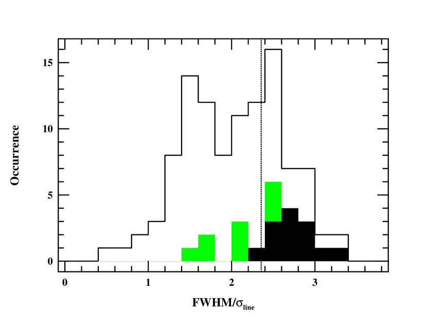
Figure 9: Distribution of values of ${\rm FWHM}/\sigma_{\rm line}$ for all lines in the rms spectra used in this analysis (i.e., columns (5) and (6) of Table 6), excluding highly uncertain values (preceeded with a colon in Table 6). The mean and standard deviation for the total distribution are $2.03\pm 0.59$. The black area shows the distribution for multiple measurements of H$\beta$ in NGC 5548 (the mean and standard deviation for this subset are $2.73\pm 0.24$). The gray area shows the distribution for other lines in NGC 5548 (mean and standard deviation for all lines in NGC 5548, including H$\beta$, are $2.45\pm 0.44$. The vertical dotted line is at ${\rm FWHM}/\sigma_{\rm line}=2.355$, which is appropriate for a Gaussian line profile. Values smaller than this indicate lines that have weaker cores and strong wings relative to a Gaussian.

For completeness, we show in Figs. 9 and 10 the distribution of the ratios ${\rm FWHM}/\sigma_{\rm line}$ and $\tau_{\rm peak}/\tau_{\rm cent}$, respectively, for all lines used in this analysis (i.e., highly uncertain values excluded). The mean and standard deviations of these distributions are ${\rm FWHM}/\sigma_{\rm line}=2.03\pm 0.59$ and $\tau_{\rm peak}/\tau_{\rm cent}=0.95\pm 0.20$. The low mean value of ${\rm FWHM}/\sigma_{\rm line}$ relative to that for a Gaussian (${\rm FWHM}/\sigma_{\rm line}=2.355$) means that, on average, these lines have weaker cores and stronger wings relative to Gaussians.

6 BLACK HOLE MASSES

For many of the objects in this study, we have multiple measurements of the virial products. In Table 8, we list for each object in this study the weighted mean virial product $<c\tau_{\rm cent}\sigma_{\rm line}^{2}/G>$, based on the entries in column (7) of Table 6, excluding the more uncertain values (those preceeded by a colon).

The masses of the central objects are given by

$$M_{\rm BH}=\frac{fc\tau_{\rm cent}\sigma_{\rm line}^{2}}{G},$$ (7)

where as noted earlier $f$ depends on the structure, kinematics, and aspect of the BLR. The scaling factor $f$ can be determined in a number of ways, the easiest being to assume that AGNs and quiescent galaxies follow the same $M_{\rm BH}$–$\sigma_{*}$ relationship; one can then use quiescent galaxy results to normalize the AGN $M_{\rm BH}$–$\sigma_{*}$ relationship and provide an absolute mass scale for AGN black holes. We carry out this exercise in a companion paper (Onken et al. 2004), in which we find $\langle f\rangle=5.5$. Our final black hole masses, based on eq. (7) with an adopted mean value $\langle f\rangle=5.5$, are given in column (3) of Table 8.

6.1 Uncertainties in Black Hole Masses

As noted earlier, the first goal of this project has been to improve the precision of the virial product measurement. We find that the typical precision (i.e., fractional error) of the virial product measurement is about 33% for the 35 AGNs for which we are able to estimate black hole masses, or $\sim 26$%, excluding NGC 4593 and IC 4329A, for which the reverberation results are notably poor. The second goal is to improve the statistical accuracy of the reverberation-based black hole mass scale using the normalization of the AGN $M_{\rm BH}$–$\sigma_{*}$ relationship reported in a companion paper (Onken et al. 2004). The scatter around the AGN $M_{\rm BH}$–$\sigma_{*}$ relationship is found to be about a factor 2.6 – 2.9, depending somewhat on the slope of the quiescent galaxy $M_{\rm BH}$–$\sigma_{*}$ relationship (Onken et al. 2004). It is important to keep in mind that this level of accuracy is statistical in nature and individual black hole masses may be less accurate.

It must be kept in mind that there are various systematic difficulties with reverberation results that can in principle lead to significant errors in individual black hole masses (e.g., Krolik 2001). Reverberation, of course, is not the only method of measuring black hole masses that can fail catastrophically under certain conditions: both stellar dynamical and gas dynamical methods can also lead to ambiguous or even misleading results (e.g., Verdoes Kleijn et al. 2000; Cappelari et al. 2003; Valluri, Merritt, & Emsellem 2004). While we find the limited scatter in the AGN $M_{\rm BH}$–$\sigma_{*}$ relationship reassuring, additional tests remain highly desirable.

6.2 On Normalization of the AGN $M_{\rm BH}-\sigma_{*}$ Relationship

As noted above, we normalize the AGN $M_{\rm BH}$–$\sigma_{*}$ relationship to the $M_{\rm BH}$–$\sigma_{*}$ relationship for quiescent galaxies by setting $f=5.5$ in eq. (7). This represents the first empirical determination of the zero point in the AGN black hole mass scale.

In previous work, the scale factor appeared in a different and more model-dependent way, only as an adjustment $\epsilon$ to the line-width parameter, i.e.,

$$\sigma=\epsilon\,\mbox{FWHM}.$$ (8)

and the virial mass is $M=c\langle\tau\rangle\sigma^{2}/G$. For example, Netzer (1990) assumed $\epsilon=\sqrt{3}/2$, which arises from assuming that $\sigma_{\rm line}=\mbox{FWHM}/2$ and that the velocity dispersion is isotropic, i.e., $\sigma=\sqrt{3}\sigma_{\rm line}$, recalling that $\sigma_{\rm line}$ is the line-of-sight velocity dispersion. This further assumes that the mean time delay $\langle\tau\rangle$ is independent of aspect or inclination, which is true when the line emission is isotropic and unabsorbed and the geometry has spherical or polar symmetry. If we make the equivalent assumptions in eq. (7), i.e., that the velocity dispersion is isotropic so $\sigma=\sqrt{3}\sigma_{\rm line}$ and that $\sigma_{\rm line}\approx\mbox{FWHM}/2$ (which is on average quite a good assumption, given the results of the previous section), then $f=3$. Our empirical calibration of the AGN mass scale through the AGN $M_{\rm BH}$–$\sigma_{*}$ relationship is thus about a factor of 1.8 ($=5.5/3$) higher than the mass scale used in previous papers (e.g., WPM and Kaspi et al. 2000). We emphasize again that the previous normalization was made only in the absence of observational information or better-justified assumptions; the value we give here is the first determination based on observational parameters, in this case as embodied in the $M_{\rm BH}$–$\sigma_{*}$ relationship.

7 COMMENTS ON SELECTED INDIVIDUAL OBJECTS

PG 0026+129.

Because of strong narrow-line residuals in the rms spectrum, we found it necessary to remove the narrow component of H$\beta$ and the [O iii] $\lambda\lambda 4959,$ 5007 lines from the individual spectra. However, the narrow lines in the vicinity of H$\alpha$ are sufficiently weak that they present no problems.

PG 0052+251.

The narrow-line components were removed from the H$\beta$ region, but the H$\alpha$ region suffers from significant narrow-line residuals in the rms spectrum. The FWHM of H$\alpha$ is untrustworthy and probably underestimated for this reason.

Fairall 9.

In this case, we used the time-binned UV continuum light curve at 1390 Å (Rodríguez-Pascual et al. 1997) as the driving light curve for all lines, including H$\beta$. Unfortunately, the C iv $\lambda 1549$ light curve is very noisy, and the cross-correlation result is not trustworthy. It is therefore excluded from the mass determination.

Mrk 590.

The H$\beta$ profile in the rms spectrum in the first data set (JD2448090–JD2448323) seems anomalously narrow, although the rms spectrum for this data set is significantly noisier than for the other rms spectra (note the lower value of $F_{\rm var}$ in Table 5). We have therefore excluded the first data set from the mass analysis, since the line width is questionable although the lag measurement seems trustworthy.

Mrk 79.

The lag measurements from the fourth data set (JD2449996–JD2450220) are not trustworthy on account of some significant aliasing effects, seen clearly in the double-peaked CCCD shown in Fig. 11. We have therefore excluded this data set.

PG 0804+761.

This is one of a handful of objects that are similar to the well-known Seyfert galaxy I Zw 1. These “I Zw 1-like” AGNs have relatively narrow lines and very strong optical Fe ii emission; they are among the more extreme members of the narrow-line Seyfert 1 (NLS1) subclass. A particular problem these objectss present is that the [O iii] $\lambda\lambda 4959$, 5007 lines are heavily contaminated by Fe ii emission, and in fact, most of the emission that makes up these features can be attributed to Fe ii $\lambda 4924$ and Fe ii $\lambda 5018$ (e.g., Peterson, Meyers, & Capriotti 1984). We are thus unable to use [O iii] $\lambda 5007$ as a template for removal of the narrow-line contaminants. However, in these cases, narrow H$\beta$ is usually too weak to strongly affect the line-width measurements, so we do not attempt narrow-line removal for these objects. In this particular quasar, there is a clear residual narrow-line H$\alpha$ component in the rms spectrum, but the line-width measurement is probably not strongly affected. On the other hand, a strong [O iii] $\lambda 4363$ residual makes H$\gamma$ highly asymmetric in the rms spectrum, and thus the line-width measurements for H$\gamma$ cannot be trusted.

PG 0844+349.

This is another I Zw 1-like object (see PG 0804+761 above). The time-lag measurements are very inconsistent from line-to-line, probably because of inadequate time sampling. There are narrow-line residuals in H$\gamma$ and H$\alpha$. The H$\beta$ cross-correlation function is clearly strongly affected by correlated errors and is thus rejected. The results on this object are of rather low quality.

Mrk 110.

The H$\beta$ data used here are from Peterson et al. (1998a). He ii $\lambda 4686$ appears as a prominent, broad feature in the rms spectra of this object, as shown in Fig. 12. We therefore constructed a light curve for He ii from the original data. Unfortunately, the He ii lags are so short that the measurements of $\tau_{\rm cent}$ and $\tau_{\rm peak}$ cannot be trusted, as they are significantly shorter than the time interval between observations. We therefore do not use the He ii lines in the mass determination, although we point out that they are generally consistent with the H$\beta$ results. Kollatschny (2003) has also studied the variability of this AGN, and finds that the results for H$\alpha$, H$\beta$, He i $\lambda 5876$, and He ii $\lambda 4686$ are consistent with a single virial mass. As discussed in more detail by Onken et al. (2004), the black-hole mass measured by Kollatschny is consistent with our measurement if we use FWHM instead of $\sigma_{\rm line}$ and Kollatschny’s value for the scaling factor $f$.

NGC 3227.

This AGN was the target of two separate optical campaigns, one by the LAG consortium in 1990 (Salamanca et al. 1994) and one at CTIO in 1992 (Winge et al. 1995). The rms spectra formed from the LAG data were recently presented by Onken et al. (2003). We completely reanalyzed the CTIO data. The original reduced spectra were rescaled in flux using the van Groningen & Wanders (1992) algorithm that has been used in most of the International AGN Watch campaigns and in the Ohio State program, and new continuum and H$\beta$ emission-line light curves were measured from the rescaled spectra. While this resulted in some improvement in the H$\beta$ lag determination and uncertainty, the rms spectrum was still quite noisy because of the combination of a low amplitude of variability and a relatively insensitive detector (see the notes on IC 4392A, below).

NGC 3516.

This is another object observed by the LAG consortium (Wanders et al. 1993). We note that the light curves for this object may be less reliable than those of other objects as the extended narrow-line region in this object makes narrow line-based flux calibration vulnerable to seeing effects, which then have to be modeled (Wanders et al. 1992). We used the scaled and corrected spectra to determine the rms spectrum, following Onken et al. (2003).

NGC 3783.

This was the second major multiwavelength campaign undertaken by the International AGN Watch (Reichert et al. 1994; Stirpe et al. 1994). This object was completely reanalyzed by Onken & Peterson (2002); new UV light curves based on IUE NEWSIPS data were measured, and the optical spectra were completely recalibrated using the van Groningen & Wanders (1992) algorithm. The results presented here are based on the Onken & Peterson reanalysis.

NGC 4051.

This object was also studied recently by Shemmer et al. (2003), who obtain a black hole mass consistent with the results of Peterson et al. (2000), who present the data we have used here.

NGC 4151.

We analyze two sets of optical data on this object, from the Wise Observatory campaign in 1988 (Maoz et al. 1991) and from the International AGN Watch project in 1993–94 (Kaspi et al. 1996). Unfortunately, the rms line profiles in the 1988 data are too poor to use due to a combination of narrow-line residuals in the rms spectra, uncertain narrow-line removal from the original spectra, and a variable line-spread function. We therefore do not use these data, except to the extent of noting that the results are broadly consistent with the later AGN Watch results; though the lag measurements appear to be reliable, the line widths in the rms spectra are not trustworthy.

PG 1211+143.

This AGN is another I Zw 1-like object (see PG 0804+761 above). Our level of confidence in the results for this object is low: the lags are suspect because the amplitude of variability is low, the variations are slow, and the time sampling is not especially good. The time lags are highly uncertain on account of this; the CCFs are very flat-topped and uncertain, as can be seen clearly in Fig. 13. Moreover, there are some problems with stability in the H$\alpha$ region of the spectrum that makes the line-width measurements of H$\alpha$ highly uncertain. Given these difficulties, we exclude this object from further analysis.

PG 1226+023.

This is the well-known quasar, 3C 273, which is another I Zw 1-like object (see PG 0804+761 above) in which the [O iii] lines are strongly blended with Fe ii lines (Peterson, Meyers, & Capriotti 1984). The narrow-line components of H$\gamma$ and H$\beta$ are weak in both the mean and rms spectra. However, there are strong narrow-line residuals in the H$\alpha$ region, so the H$\alpha$ line-width measurements cannot be trusted.

PG 1229+204.

Inspection of the light curves shows that the variations in this object are not well sampled. The large differences in lags for the Balmer lines make the results on this object rather dubious. We have low confidence in the results for this object.

NGC 4593.

This is another object from the LAG campaign in 1990 (Dietrich et al. 1994), where the data have been reanalyzed by Onken et al. (2003). We regard the H$\beta$ lag as completely unreliable because it is so much smaller than the mean sampling interval. The H$\alpha$ lag should also be regarded with some caution.

PG 1307+085.

The H$\alpha$ region of the rms spectrum in this object shows residual narrow-line H$\alpha$, though this probably affects only the FWHM measurement.

IC 4329A.

This object and NGC 3227 were both observed in the CTIO monitoring program (Winge et al. 1995, 1996). These observations employed a Reticon detector, which yielded poorer quality spectra than obtained with the CCDs used in virtually every other ground-based campaign. We attempted to improve the original lightcurves by rescaling the original spectra in flux by using the van Groningen & Wanders (1992) algorithm and remeasuring the continuum and emission-line fluxes. This did improve light curves and rms spectra, but only marginally. The light curves are very poor and the time-lag measurements should be regarded with caution. The FWHM measurement is very poor (note the large uncertainty yielded by our measurement algorithm). We have little confidence in the mass determination for this object.

Mrk 279.

We examined two completely independent sets of data, one from the Wise Observatory program in 1988 (Maoz et al. 1990) and one from an International AGN Watch project in 1996 (Santos-Lleó et al. 2001). The AGN Watch data appear to be quite good. The Wise Observatory data, however, have a number of problems: the CCFs for both H$\alpha$ and H$\beta$ show a correlated error signal at zero lag; this problem is particularly bad at H$\beta$, and we will therefore not use the H$\beta$ lag measurements. Furthermore, the H$\alpha$ region of the rms spectrum is strongly contaminated by narrow-line residuals, and H$\beta$ is so weak that the FWHM measurement is meaningless. Nevertheless, the mass determination is quite consistent with the results of the AGN Watch program.

NGC 5548.

Some comments on this object appear in section 5. There are more published variability data, by far, on this object than any other, and most of the data are very good. Only a few problems need to be pointed out. First, the H$\alpha$ region of the rms spectrum from the Wise Observatory campaign (Netzer et al. 1990) has strong narrow-line residuals that render the line-width measures unusable. The CCCD for the associated time series is also rather ambiguous, so we do not include these measurements in the mass determination. The H$\beta$ profile in the rms spectrum from the fifth year of AGN Watch monitoring (i.e., JD2448954–JD2449255) is very unusual, as shown in Fig. 14; there are two peaks, a strong central peak and a weak blue peak. The FWHM measurement is thus meaningless. Finally, He ii $\lambda 4686$ is prominent in the rms spectrum for the first year of the AGN Watch campaign (JD2447509–JD2447809), but is too heavily blended with the optical Fe ii blends to measure in the mean spectrum; this line is not included in this part of the analysis (cf. Figs. 4 and 5).

PG 1700+518.

The CCCD for this object shows two peaks, one of them clearly ascribable to correlated errors in the continuum and emission-line light curves (Fig. 15). Fortunately, the peaks are well-separated, and we can exclude the zero-lag correlated error peak from our analysis. This significantly increases the H$\beta$ lag and also the black hole mass relative to the original investigation by Kaspi et al. (2000).

3C 390.3.

Some of the difficulties with this object have already been discussed in section 5. Part of the problem with these data seems to be just the nature of the variability: apart from a large-scale outburst during the early part of the monitoring campaign, the variations were very weak. As noted earlier, the lines are very broad and blended, and the most consistent black hole mass is obtained by using the line width measured from the unblended side of each line and then assuming symmetry. A more detailed attempt at deconvolution might improve this. Finally, we note that in this case, we used the UV continuum (at 1370 Å) as the driving continuum in the cross-correlation analysis.

Mrk 509.

Like Mrk 110, the He ii $\lambda 4686$ line is prominent in the rms spectrum of this object, so we therefore attempted to measure it in each spectrum and produce a light curve. Because of blending with optical Fe ii emission, the resulting light curve is probably not as reliable as the H$\beta$ light curve.

NGC 7469.

This object is one of a very few in which a lag has been detected between the UV and optical continuum variations (Wanders et al. 1997; Collier et al. 1998). We therefore in this case use the UV continuum (at 1315 Å) as the driving continuum in the cross-correlation analysis.

8 THE MASS–LUMINOSITY RELATIONSHIP

Our improved database can be used to investigate the relationships between BLR radius and luminosity and black hole mass and luminosity. The radius–luminosity relationship is discussed in a companion paper (Kaspi et al. 2004), and here we will discuss only the mass–luminosity relationship.

We computed the optical luminosity from the flux measurements in the original data sources that were made over the time intervals used in this analysis. In each case, we selected the continuum waveband closest to 5100 Å in the AGN rest frame. We corrected for Galactic reddening using the extinction values in column (7) of Table 1 and using the reddening curve of Savage & Mathis (1979), adjusted to $A_{V}/E(B-V)=3.2$. Luminosity distances were computed using the redshifts given in column (5) of Table 1 and by assuming a standard flat $\Lambda$CDM cosmology with $\Omega_{\rm B}=0.04$, $\Omega_{\rm DM}=0.26$, $\Omega_{\Lambda}=0.70$, and $H_{\rm o}=70$ km s^-1 Mpc^-1. For AGNs with multiple mass determinations, we computed the average value of $\log\lambda L_{\lambda}$ from each individual time series. The optical luminosities $\log\lambda L_{\lambda}$ are given in column (4) of Table 8. The corresponding uncertainties represent the amplitude of continuum variability during the reverberation experiment.

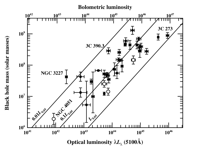
Figure 16: Black hole mass vs. luminosity for 35 reverberation mapped AGNs. The luminosity scale on the lower x-axis is $\log\lambda L_{\lambda}$ in units of ergs s^-1. The upper x-axis shows the bolometric luminosity assuming that $L_{\rm bol}\approx 9\lambda L_{\lambda}$. The diagonal lines show the Eddington limit $L_{\rm Edd}$, $0.1L_{\rm Edd}$, and $0.01L_{\rm Edd}$. The open circles represent NLS1s. Other labeled points are discussed in the text.

In Fig. 16, we plot the reverberation-based masses we have derived as a function of the mean luminosity. This figure can be compared directly with Fig. 8 of Kaspi et al. (2000), which reveals that a much better-defined mass–luminosity relationship results from our improved analysis. We have also estimated the bolometric luminosity in the same fashion as Kaspi et al., i.e., $L_{\rm bol}\approx 9\lambda L_{\lambda}(5100\,{\rm\AA})$, and this scale is shown on the top of Fig. 16. The diagonal lines show the Eddington limit, and 10% and 1% its value.

We note that this constitutes only a preliminary version of the mass–luminosity relationship, for comparison with earlier work. A more exhaustive study of this relationship is continuing. Several comments are in order:

1. It is reassuring that there are no objects above the Eddington limit (i.e., to the right of the diagonal line), in contrast to the results of Kaspi et al. This is because our analysis has corrected a number of errors in earlier work, most notably removal of residual narrow-line H$\beta$ from many of the rms spectra, which resulted in larger line widths and rather higher overall black hole masses. The object closest to the Eddington limit is, not surprisingly, 3C 273 (PG 1226+023).

2. The bolometric correction we have assumed is nominal, based on a spectral energy distribution (SED) with a strong blue bump. However, observed SEDs suggest that a smaller ratio, e.g., $L_{\rm bol}\approx 5\lambda L_{\lambda}$ (Netzer 2003), may be on average more appropriate. Moreover, the bolometric correction we adopt may not be appropriate for all types of AGNs at arbitrary luminosity. The bolometric luminosities are thus uncertain and should be treated with some caution.

3. The optical luminosities used here have not been corrected for the contribution of starlight from the host galaxies. This can be a significant factor, especially in the lower-luminosity objects. For example, the standard aperture used in the NGC 5548 optical monitoring program, 5${}^{\prime\prime}\!.$0 $\times$ 7${}^{\prime\prime}\!.$5, admits a starlight flux of $F_{\lambda}(5100\,{\rm\AA})\approx 3.4\times 10^{-15}$ ergs s^-1 cm^-2 Å^-1 (Romanishin et al. 1995). Correcting for this reduces the optical luminosity entry for NGC 5548 in Table 8 by $\sim 0.24$ dex. A program is currently underway to determine the starlight contribution to the optical luminosity of each of these objects.

4. Internal extinction has not been accounted for in any way. Correction for extinction will move objects to the right in this diagram. It is worth noting that the object with the lowest Eddington rate (farthest to the left of the $0.01L_{\rm Edd}$ diagonal) is NGC 3227, which is a rather dusty object (Pogge & Martini 2002). The low luminosity of this object relative to its black hole mass may be a result of internal extinction.

5. Given the small formal error bars for most of the objects, we believe that much of the scatter in Fig. 16 is real. Moreoever, we find that the scatter correlates with other AGN properties; the I Zw 1-type objects generally lie along the bottom edge of the envelope defined by the data points. In Fig. 16, the NLS1s are shown as open circles, and all of them except NGC 4051 lie on the lower edge of the mass–luminosity envelope. Conversely, the one object with strongly double-peaked Balmer line profiles, 3C 390.3, lies along the upper edge of the envelope. The locations of these extreme objects on this diagram suggest that at least some of the dispersion of the data points correlates with Eigenvector 1, consistent with the suggestion originated by Boroson & Green (1992) and reaffirmed by numerous later authors that Eigenvector 1 appears to be driven by Eddington ratio $\dot{m}=\dot{M}/\dot{M}_{\rm Edd}$. However, the physical origin of the scatter observed in Fig. 16 could be attributable either to differences in Eddington ratio or to inclination effects. Decreasing inclination (i.e., from edge-on to face-on) will translate points to the right as the apparent luminosity increases on account of decreased limb darkening and downward as the rotational velocities appear to decrease. Increasing the Eddington ratio will translate points in the same sense.

6. The best fit mass-luminosity relationship is found to be

   $$\log\left(M/10^{8}\,M_{\odot}\right)=-0.12(\pm 0.07)+0.79(\pm 0.09)\log\left(\lambda L_{\lambda}(5100\,{\rm\AA})/10^{44}\,{\rm erg\,s}^{-1}\right).$$ (9)

   However, there is no reason to believe that there are no selection effects operating. Interestingly, the lower edge of the envelope seems to parallel the lines of constant Eddingtion ratio rather well, suggesting that the intrinsic mass–luminosity slope may not differ signficantly from unity.

9 SUMMARY

In this contribution, we have improved the calibration of the reverberation-based AGN black hole mass scale by decreasing random and systematic errors and by drawing on the AGN $M_{\rm BH}$–$\sigma_{*}$ relationship to establish a statistically accurate calibration that is tied to other methods of black hole mass measurement. We have undertaken a consistent reanalysis of a highly inhomogeneous database that consists of 117 separate time series, not including several others that were deemed to be too poor to use, in the process accounting for a variety of systematic effects such as time dilation on the time lags and spectral resolution on the line widths. Each time series is treated independently and yields an independent estimate of the black hole mass, thus reducing random uncertainties. Poor or suspicious data are removed from the database, noting especially the susceptibility of time-lag measurements to correlated errors and other types of aliasing. We find that the most consistent mass measurements are obtained by using the cross-correlation centroid $\tau_{\rm cent}$ to characterize the light-travel time across the BLR and by using the line dispersion $\sigma_{\rm line}$ as measured in the rms spectrum to characterize the velocity dispersion of the BLR. In practice, special care has been taken to remove residual narrow-line contamination of the rms spectrum in cases where it is present. The result of this analysis is a revised AGN mass scale based on 35 reverberation-mapped AGNs that is statistically accurate to better than a factor of three.

Appendix A SOME COMMENTS ON CROSS-CORRELATION METHODOLOGY

Welsh (1999) has suggested a number of modifications to our error analysis procedures and we have investigated these through additional Monte Carlo simulations similar to those described by P98b.

Emission-line lag measurements are made by cross-correlating the emission-line and continuum light curves. Since the data are almost never regularly sampled, real data points in one time series are matched with values obtained by linear interpolation of the other time series. The cross-correlation function (CCF) is measured twice, once interpolating in the continuum series, and once in the emission-line series, and the final CCF is determined by averaging these two results. The CCF is characterized by (1) its peak value (highest value of the correlation coefficient) $r_{\rm max}$, (2) the time delay corresponding to this value $\tau_{\rm peak}$, and (3) the centroid $\tau_{\rm cent}$ of the peak in the CCF. In practice, $\tau_{\rm cent}$ is evaluated using only points with values about some threshold, usually $0.8r_{\rm max}$.

To assess the uncertainties in the determination of $\tau_{\rm peak}$ and $\tau_{\rm cent}$, we use the model-independent Monte Carlo FR/RSS method described by P98b. For each Monte Carlo realization, we start with a parent light curve of $N$ data points and from this make $N$ independent random selections of these data points without consideration for previous selections. The redundant selections are then discarded, leaving a new light curve of $M\leq N$ points; typically, the fraction of points from the parent light curve that remain unselected in each realization is $\sim 1/e$. We refer to this process as “random subset selection” (RSS), and it seems to successfully account for uncertainties due to effects of individual data points. Another major source of uncertainty is the uncertainty in the measured continuum and emission-line fluxes, and these can be significant if the amplitude of variability is not much larger than the flux errors in individual data points. We attempt to account for this by altering the fluxes of the $M$ data points in each Monte Carlo realization by random Gaussian deviates scaled by the flux error associated with the data point. We refer to this process as “flux randomization” (FR). This process is repeated for many independent realizations (usually 2000 or more for the light curves analyzed here), and for the CCF from each realization, $r_{\rm max}$, $\tau_{\rm peak}$, and $\tau_{\rm cent}$ are recorded. These are used to build up “cross-correlation peak distributions (CCPDs)” and “cross-correlation centroid distributions (CCCDs)” for $\tau_{\rm peak}$ and $\tau_{\rm cent}$, respectively. This is done because the distributions of these values are rarely even approximately Gaussian (Maoz & Netzer 1989).

Welsh (1999) points out a number of potential problems with cross-correlation methodology, some of which can produce biases in determination of the emission-line lags. However, simulations that mimic as much as possible real AGN behavior have not revealed any strong systematic biases. Nevertheless, we caution that cross-correlation of light curves to measure emission-line lags is a rather crude tool, but one that seems to be effective with the limited AGN variability data available at present. Welsh has also suggested a number of modification to the FR/RSS method, and we have extended the Monte Carlo simulations described by P98b to test these suggestions under what we regard as reasonably realistic conditions, and we describe our results below.

Flux Uncertainties and Redundant Selections.

Welsh (1999) suggests an alternative strategy to FR/RSS, namely counting redundant selections in each realization and appropriately reducing the flux error for multiply-selected points. Specifically, the flux uncertainty for each point that is selected $1\leq n\leq N$ times should be reduced by a factor of $n^{1/2}$. Thus, rather than omitting redundant points, each of the $N$ selections has some real effect on the outcome of the realization and the weighting is more consistent with the standard bootstrap method (e.g., Diaconis & Efron 1983) on which the FR/RSS method is based. We carried out detailed simulations like those described by P98b to determine the efficacy of Welsh’s proposed scheme. We compare different error assessments by examining the width of the CCPDs and CCCDs produced by simulations; we presume that the algorithm that yields the narrowest CCPDs and CCCDs (i.e., the highest precision measurements) is the best, as long as the errors are not underestimated. Our simulations confirm that the error estimates using Welsh’s method are superior to those of the original FR/RSS algorithm. The uncertainties in $\tau_{\rm peak}$ are typically lower by $\sim 8$%, and the uncertainties in $\tau_{\rm cent}$ are lower by $\sim 3$%. Following the procedures of P98b, we have also carried out model-dependent Monte Carlo simulations in which we use a known model for the transfer function in order to verify that Welsh’s algorithm does not underestimate the uncertainties. We therefore adopt this improvement in the cross-correlation analysis employed in this contribution.

Detrending the Light Curves.

Welsh (1999) also suggests that cross-correlation results are more accurate if the data are first “detrended,” i.e., a low-order (usually linear) polynomial is fitted to the light curve and subtracted off prior to carrying out the cross-correlation analysis. Our simulations support this, but only in the case where the sampling is excellent, i.e., long duration at high resolution (for the cases considered by P98b, say, a 200-day experiment with observations once per day). However, we find that under conditions of more marginal sampling (say, a 200-day experiment with only 40 observations), which includes nearly all reverberation data that exist, detrending either makes little difference or can, in fact, lead to occasional gross errors in the lag determination and, consequently, gross overestimates of the uncertainties in the lags. For this reason, we elect to not detrend our data prior to cross-correlation.

Peak or Centroid?

Whether or not the cross-correlation lag is better characterized by the peak or centroid of the CCF has been debated on many occasions. The advantage of the centroid is that it is related to the centroid of the transfer function and is better defined when the CCF has a broad peak, and for these reasons, we prefer it. Welsh’s simulations, however, suggest that the peak is a more robust measure than the centroid, quite at odds with what was found by P98b and contrary to our general experience. The difference seems to be attributable to differences in the transfer functions used by Welsh and by P98b; P98b used only thin-shell and thick-shell transfer functions which are flat-topped (i.e., with poorly defined peaks), whereas Welsh used only Gaussian transfer functions. If we repeat the simulations of P98b with Gaussian transfer functions, we find little reason to prefer one measure to the other. Further investigation of this issue using real data, as described in this paper, leads us to continue to prefer the CCF centroid, although the CCD peak is also an acceptable way to characterize the emission-line lags.

Centroid Threshold.

Aliasing effects can lead to complex structures in CCFs; rarely is the principal peak in the CCF isolated and well-defined. It is therefore necessary to compute the CCF centroid only over a restricted range, including points with values larger than some fixed fraction of the peak value $r_{\rm max}$. It is conventional to use a threshold of $0.8r_{\rm max}$ for this computation, although in some cases where the peak is noisy, lower thresholds are used. In some cases, the centroid can vary significantly for different threshold selections (Koratkar & Gaskell 1991), though this appears to be less of a problem with well-sampled data (e.g., Dietrich et al. 1993). Simulations based on those of P98b, however, show that a threshold value of $0.8r_{\rm max}$ is generally a good choice. With lower thresholds, we find that the CCCD is significantly broadened. For a threshold of $0.5r_{\rm max}$, for example, we find that the width of the CCCD increases by 10–20%, depending somewhat on the details of the transfer function (i.e., more sharply peaked transfer functions give results less sensitive to the selected threshold value, as one might expect). We will therefore continue to use a threshold of $0.8r_{\rm max}$, unless otherwise noted.

Figure 1: Measurement of FWHM for double-peaked profiles. A continuum is interpolated underneath the line profile and is subtracted from the data. Peak fluxes are identified on the short-wavelength and long-wavelength peaks, $P(\lambda)_{max,short}$ and $P(\lambda)_{max,long}$, respectively. On each side of the line, wavelengths corresponding to the half-maximum fluxes $0.5P(\lambda)_{max,short}$ and $0.5P(\lambda)_{max,long}$ are found moving upward from the continuum at $\lambda_{1}$ and downward from the peak at $\lambda_{2}$. In this example, $\lambda_{1}=\lambda_{2}$ on the short-wavelength side only. The nominal position of the half-maximum point is taken to be the average of $\lambda_{1}$ and $\lambda_{2}$.

Figure 2: Comparison of FWHM measurements and uncertainties from this paper with those from WPM. For the sake of meaningful comparison, the new measurements here have not been corrected for spectral resolution, as have all other line-width measurements in this paper.

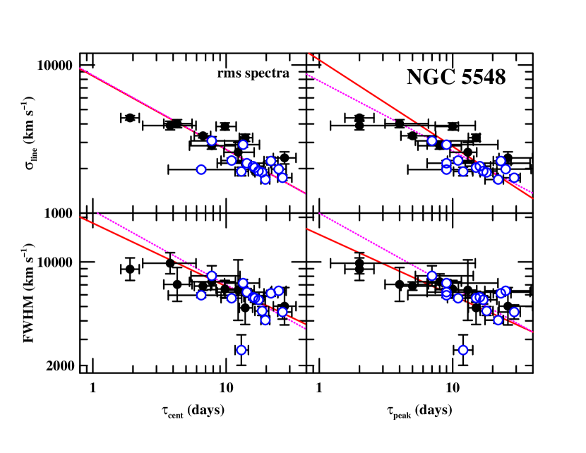
Figure 3: Line widths versus time lags for emission lines in the rms spectra of NGC 5548. The top row shows the line dispersion $\sigma_{\rm line}$ as a line width measure, and the bottom row shows FWHM. The left column shows the CCF centroid $\tau_{\rm cent}$ as the time-lag measure and the right column shows the location of the CCF peak $\tau_{\rm peak}$. The solid line is the best fit to the data, and the dotted line is a forced fit to slope $-1/2$, the virial slope. The fit parameters are summarized in Table 7. The open circles are measurements of H$\beta$ for 14 different years. The filled circles represent all of the other lines.

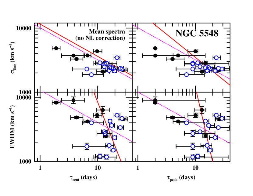
Figure 4: Line width versus time lags for emission lines in the mean spectra of NGC 5548. The data are plotted as in Fig. 3. Note the dramatic change in the scatter, especially for the H$\beta$ line, by using the mean rather than the rms line profile for the line-width measurement.

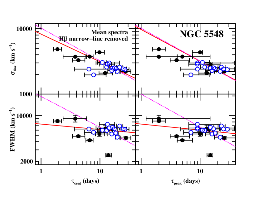
Figure 5: Line widths versus time lags for emission lines in the mean spectra of NGC 5548, but with the narrow component of H$\beta$ removed. The data are plotted as in Figs. 3 and 4. Removing the narrow-component of H$\beta$ greatly reduces the scatter around the virial relationship, but the scatter is still much more pronounced than in Fig. 3, where the line-widths are measured in the rms profiles. The measurement uncertainties on $\sigma_{\rm line}$ are too small to show up on this diagram. Note that the fits to the data in the lower panel are unweighted fits on account of the large number of outliers.

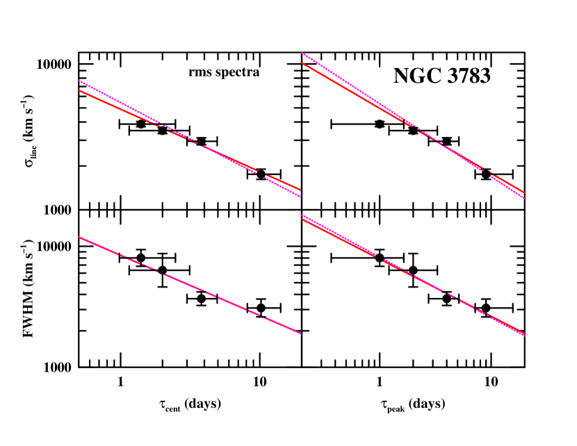
Figure 6: Line widths versus time lags for emission lines in the rms spectra of NGC 3783. The data are plotted as in Fig. 3.

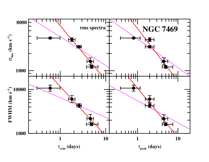
Figure 7: Line widths versus time lags for emission lines in the rms spectra of NGC 7469. The data are plotted as in Fig. 3.

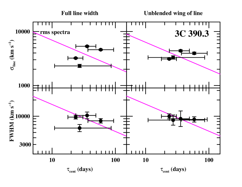
Figure 8: Line width versus CCF centroid $\tau_{\rm cent}$ for emission lines in the rms spectra of 3C 390.3. The top row shows the line dispersion $\sigma_{\rm line}$ used as the line-width measure, and the bottom row shows FWHM. The left-hand column shows our standard line-width measurement, using the whole line, but with no effort to account for blending. In the right-hand column, we attempt to account for blending by measuring the unblended half of each line. In any case, the large uncertainties in the time lags preclude a critical test of a virial relationship.

Figure 10: Distribution of values of $\tau_{\rm peak}/\tau_{\rm cent}$ for all lines in this analysis (i.e., columns (3) and (4) of Table 6), excluding highly uncertain values (preceeded with a colon in Table 6). The mean and standard deviation for this distribution are $0.95\pm 0.20$.

Figure 11: Cross-correlation centroid distribution for the continuum–H$\beta$ cross-correlation for Mrk 79 during the period JD2449996 to JD2450220. It is not obvious which peak corresponds to the correct lag.

Figure 12: Mean (top panel) and rms (bottom panel) spectra of Mrk 110. The rms spectrum shows clearly the very broad He ii $\lambda 4686$ and broad H$\beta$. The narrow [O iii] $\lambda\lambda 4959$, 5007 lines appear only in the mean spectrum, except for weak residuals in [O iii] $\lambda 5007$ that appear in the rms spectrum.

Figure 13: Cross-correlation functions for PG 1211+143. The dotted line is the H$\alpha$ CCF, the solid line is the H$\beta$ CCF, and the dashed line is the H$\gamma$ CCF. The centroids and peaks are poorly defined because the CCFs are broad and flat-topped.

Figure 14: Mean (top panel) and rms (bottom panel) H$\beta$-region spectra of NGC 5548 during the period JD2448954 to JD2449255, the fifth year of monitoring by the International AGN Watch (1993). The H$\beta$ profile in the rms spectrum is double-peaked; there is a strong peak at line center and another in the shortward wing of the line.

Figure 15: Cross-correlation centroid distribution for the continuum–H$\beta$ cross-correlation for PG 1700+518. The peak at zero lag is clearly ascribable to correlated error, so it can be rejected.

Table 1: Object List

		$\alpha_{2000}$	$\delta_{2000}$	$z$	$V$	$A_{B}$	Véron-Cetty & Véron	Alternative
Objects	References	(hr min sec)	(${}^{\rm o}\ {}^{\prime}\ {}^{\prime\prime}$)		(mag)	(mag)	Catalog Name	Name
(1)	(2)	(3)	(4)	(5)	(6)	(7)	(8)	(9)
Mrk 335	1	$00\ 06\ 19.521$	$+20\ 12\ 10.49$	0.02578	13.7	0.153	J000619.5$+$201211	PG 0003$+$199
PG 0026$+$129	2	$00\ 29\ 13.600$	$+13\ 16\ 03.00$	0.14200	15.4	0.307	J002913.8$+$131605
PG 0052$+$251	2	$00\ 54\ 52.100$	$+25\ 25\ 38.00$	0.15500	15.4	0.205	J005452.2$+$252539
Fairall 9	3,4	$01\ 23\ 45.780$	$-58\ 48\ 20.50$	0.04702	13.5	0.116	J012345.8$-$584821
Mrk 590	1	$02\ 14\ 33.562$	$-00\ 46\ 00.09$	0.02638	13.8	0.161	J021433.6$-$004600	NGC 863
3C 120	1	$04\ 33\ 11.095$	$+05\ 21\ 15.62$	0.03301	14.1	1.283	J043311.1$+$052115	Mrk 1506
Akn 120	1	$05\ 16\ 11.421$	$-00\ 08\ 59.38$	0.03230	14.1	0.554	J051611.4$-$000900	Mrk 1095
Mrk 79	1	$07\ 42\ 32.797$	$+49\ 48\ 34.75$	0.02219	13.9	0.305	J074232.8$+$494835
PG 0804$+$761	2	$08\ 10\ 58.600$	$+76\ 02\ 42.00$	0.10000	15.1	0.150	J081058.5$+$760243
PG 0844$+$349	2	$08\ 47\ 42.400$	$+34\ 45\ 04.00$	0.06400	14.0	0.159	J084742.5$+$344505
Mrk 110	1	$09\ 25\ 12.870$	$+52\ 17\ 10.52$	0.03529	16.0	0.056	J092512.9$+$521711
PG 0953$+$414	2	$09\ 56\ 52.400$	$+41\ 15\ 22.00$	0.23410	14.5	0.054	J095652.3$+$411522
NGC 3227	5,6,7	$10\ 23\ 30.589$	$+19\ 51\ 53.99$	0.00386	11.1	0.098	J102330.6$+$195156
NGC 3516	6,8	$11\ 06\ 47.490$	$+72\ 34\ 06.88$	0.00884	12.5	0.183	J110647.4$+$723407
NGC 3783	9,10,11	$11\ 39\ 01.77$	$-37\ 44\ 18.7$	0.00973	12.6	0.514	J113901.8$-$374419
NGC 4051	12	$12\ 03\ 09.614$	$+44\ 31\ 52.80$	0.00234	10.8	0.056	J120309.6$+$443153
NGC 4151	13,14	$12\ 10\ 32.579$	$+39\ 24\ 20.63$	0.00332	11.5	0.119	J121032.5$+$392421
PG 1211$+$143	2	$12\ 14\ 17.700$	$+14\ 03\ 12.60$	0.08090	14.6	0.150	J121417.7$+$140313
PG 1226$+$023	2	$12\ 29\ 06.700$	$+02\ 03\ 08.60$	0.15834	12.8	0.089	J122906.7$+$020308	3C 273
PG 1229$+$204	2	$12\ 32\ 03.605$	$+20\ 09\ 29.21$	0.06301	15.3	0.117	J123203.6$+$200930	Mrk 771
								Ton 1542
NGC 4593	6,15	$12\ 39\ 39.425$	$-05\ 20\ 39.34$	0.00900	11.7	0.106	J123939.4$-$052039	Mrk 1330
PG 1307$+$085	2	$13\ 09\ 47.000$	$+08\ 19\ 48.90$	0.15500	15.3	0.145	J130947.0$+$081949
IC 4329A	16	$13\ 49\ 19.29$	$-30\ 18\ 34.4$	0.01605	14.0	0.255	J134919.3$-$301834
Mrk 279	17,18	$13\ 53\ 03.447$	$+69\ 18\ 29.57$	0.03045	14.6	0.068	J135303.5$+$691830
PG 1351$+$640	2	$13\ 53\ 15.808$	$+63\ 45\ 45.41$	0.08820	14.8	0.088	J135315.7$+$634546
PG 1411$+$442	2	$14\ 13\ 48.300$	$+44\ 00\ 14.00$	0.08960	15.0	0.036	J141348.3$+$440014
NGC 5548	19,20,21,22,23	$14\ 17\ 59.534$	$+25\ 08\ 12.44$	0.01717	13.3	0.088	J141759.6$+$250813
PG 1426$+$015	2	$14\ 29\ 06.588$	$+01\ 17\ 06.48$	0.08647	17.5	0.137	J142906.5$+$011704	Mrk 1383
Mrk 817	1	$14\ 36\ 22.068$	$+58\ 47\ 39.38$	0.03145	14.5	0.029	J143622.1$+$584740	PG 1434$+$590
PG 1613$+$658	2	$16\ 13\ 57.179$	$+65\ 43\ 09.58$	0.12900	15.2	0.114	J161357.2$+$654309	Mrk 876
PG 1617$+$175	2	$16\ 20\ 11.288$	$+17\ 24\ 27.70$	0.11244	15.5	0.180	J162011.3$+$172428	Mrk 877
PG 1700$+$518	2	$17\ 01\ 24.800$	$+51\ 49\ 20.00$	0.29200	15.4	0.151	J170125.0$+$514920
PG 1704$+$608	2	$17\ 04\ 41.370$	$+60\ 44\ 30.50$	0.37100	15.3	0.097	J170441.5$+$604428
3C390.3	24,25	$18\ 42\ 08.9899$	$+79\ 46\ 17.127$	0.05610	14.4	0.308	J184209.0$+$794617
Mrk 509	1	$20\ 44\ 09.738$	$-10\ 43\ 24.54$	0.03440	13.0	0.248	J204409.7$-$104324
PG 2130$+$099	2	$21\ 32\ 27.813$	$+10\ 08\ 19.46$	0.06298	14.6	0.192	J213227.8$+$100819	II Zw 136
								Mrk 1513
NGC 7469	26,27	$23\ 03\ 15.623$	$+08\ 52\ 26.39$	0.01632	13.0	0.297	J230315.6$+$085226	Mrk 1514

Table 2: Wavelength Windows for Line Width Measurements

		Data	Res.	Julian Dates	Continuum	Continuum	Line
Object	Ref.	Set	(Å)	(-2400000)	Window (Å)	Window (Å)	Limits (Å)
(1)	(2)	(3)	(4)	(5)	(6)	(7)	(8)
Mrk 335	1	H$\beta$	9.6	49156–49338	4900–4910	5095–5105	4930–5030
	1	H$\beta$	9.6	49889–50118	4910–4920	5100–5110	4930–5030
PG 0026+129	2	H$\alpha$	12.5	48836–51084	7290–7300	7700–7740	7304–7728
	2	H$\beta$	12.5	48545–51084	5442–5450	5820–5840	5460–5700
PG 0052+251	2	H$\alpha$	12.5	48837–51084	7028–7108	7725–7800	7398–7724
	2	H$\beta$	12.5	48461–51084	5418–5488	5908–5978	5518–5698
	2	H$\gamma$	12.5	48461–51084	4864–4914	5418–5488	4926–5118
Fairall 9	3	H$\beta$	11.2	50473–50665	4936–4946	5295–5323	4946–5295
	4	C iv $\lambda 1549$	6.0	50473–50713	1540–1565	1760–1770	1565–1670
	4	Ly$\alpha$	6.0	50473–50713	1227–1232	1370–1380	1232–1334
Mrk 590	1	H$\beta$	9.6	48090–48323	4940–4955	5050–5065	4965–5045
	1	H$\beta$	9.6	48848–49048	4880–4890	5235–5245	4890–5095
	1	H$\beta$	9.6	49183–49338	4930–4935	5165–5170	4955–5069
	1	H$\beta$	9.6	49958–50122	4920–4930	5170–5180	4930–5068
3C 120	1	H$\beta$	9.6	47837–50388	4958–4972	5100–5108	4972–5100
Akn 120	1	H$\beta$	9.6	48148–48344	4910–4920	5246–5255	4920–5107
	1	H$\beta$	9.6	49980–50175	4910–4920	5245–5255	4920–5102
Mrk 79	1	H$\beta$	9.6	47838–48044	4795–4810	5190–5210	4850–5040
	1	H$\beta$	9.6	48193–48393	4850–4870	5075–5085	4890–5040
	1	H$\beta$	9.6	48905–49135	4880–4885	5080–5086	4885–5040
	1	H$\beta$	9.6	49996–50220	4830–4840	5050–5060	4840–5040
PG 0804+761	2	H$\alpha$	12.5	48319–51085	6746–6814	7472–7520	6940–7412
	2	H$\beta$	12.5	48319–51085	5224–5264	5598–5630	5266–5474
	2	H$\gamma$	12.5	48319–51085	4680–4705	4880–4905	4710–4850
PG 0844+349	2	H$\alpha$	12.5	48319–51085	6708–6764	7248–7348	6848–7120
	2	H$\beta$	12.5	48319–51085	5048–5078	5414–5440	5098–5248
	2	H$\gamma$	12.5	48319–51085	4503–4535	4710–4750	4536–4690
Mrk 110	1	H$\beta$	9.6	48953–49149	4970–4980	5090–5100	4980–5090
	1	H$\beta$	9.6	49751–49874	4715–4740	5250–5260	4975–5066
	1	H$\beta$	9.6	50010–50262	4965–4970	5150–5160	4975–5070
	1	He ii $\lambda 4686$	9.6	48953–49149	4730–4740	4970–4980	4740–4970
	1	He ii $\lambda 4686$	9.6	49751–49874	4740–4750	5240–5260	4750–4965
	1	He ii $\lambda 4686$	9.6	50010–50262	4750–4760	4960–4970	4760–4960
PG 0953+414	2	H$\beta$	12.5	48319–50997	5846–5892	6288–6320	5909–6086
	2	H$\gamma$	12.5	48319–50997	5238–5278	5472–5506	5284–5450
NGC 3227	5,6	H$\alpha$	9.1	47894–48045	6420–6430	6800–6830	6430–6780
	5,6	H$\beta$	9.1	47894–48049	4780–4795	5115–5120	4800–4955
	7	H$\beta$	11.2	48623–48776	4765–4785	5085–5100	4800–4940
NGC 3516	6,8	H$\alpha$	9.1	47894–48047	6426–6477	6820–6850	6477–6820
	6,8	H$\beta$	9.1	47894–48047	4782–4807	5175–5195	4807–5031
NGC 3783	9,10	H$\beta$	11.2	48607–48833	4800–4810	5128–5160	4810–4984
	10,11	Si iv $\lambda 1400$	6.0	48611–48833	1363–1373	1464–1470	1373–1450
	10,11	C iv $\lambda 1549$	6.0	48611–48833	1464–1470	1710–1725	1509–1613
	10,11	He ii $\lambda 1640$	6.0	48611–48833	1464–1470	1710–1725	1613–1709
NGC 4051	12	H$\beta$	9.6	50183–50263	4810–4820	4915–4930	4835–4910
	12	He ii $\lambda 4686$	9.6	50183–50263	4570–4600	4745–4760	4610–4740
NGC 4151	13	H$\beta$	12.5	49305–49404	4785–4795	4946–4954	4795–4945
	13	H$\alpha$	12.5	49305–49404	6200–6250	6790–6810	6360–6737
	14	H$\beta$	13.3	47145–47360	4767–4775	5090–5100	4775–4923
	14	H$\alpha$	13.3	47145–47360	6400–6430	6682–6690	6440–6682
PG 1211+143	2	H$\alpha$	12.5	48319–51000	6670–6720	7480–7540	6900–7310
	2	H$\beta$	12.5	48319–51000	5120–5160	5490–5530	5180–5340
	2	H$\gamma$	12.5	48319–51000	4525–4560	4780–4810	4625–4755
PG 1226+023	2	H$\alpha$	12.5	48361–50997	7034–7085	7789–7808	7250–7788
	2	H$\beta$	12.5	48361–50997	5494–5522	5888–5928	5530–5756
	2	H$\gamma$	12.5	48361–50997	4925–4945	5135–5165	4946–5130
PG 1229+204	2	H$\alpha$	12.5	48319–50997	6562–6654	7244–7320	6838–7148
	2	H$\beta$	12.5	48319–50997	5052–5088	5412–5456	5094–5244
	2	H$\gamma$	12.5	48986–50997	4500–4560	4694–4758	4560–4690
NGC 4593	6,15	H$\alpha$	9.1	47894–48049	6450–6470	6735–6760	6510–6710
	6,15	H$\beta$	9.1	47894–48049	4745–4790	5105–5130	4828–4961
PG 1307+085	2	H$\alpha$	12.5	49130–51000	7050–7100	7750–7800	7400–7740
	2	H$\beta$	12.5	48319–51042	5458–5488	5864–5914	5508–5698
	2	H$\gamma$	12.5	48319–51042	4870–4915	5104–5154	4938–5088
IC 4329A	16	H$\beta$	11.5	48643–48832	4780–4850	5160–5200	4850–5060
Mrk 279	17	H$\beta$	9.6	50095–50289	4940–4950	5185–5200	4950–5090
	18	H$\beta$	13.3	47205–47360	4840–4880	5270–5300	4950–5090
	18	H$\alpha$	13.3	47205–47360	6520–6600	6878–6882	6688–6878
PG 1411+442	2	H$\alpha$	12.5	48319–51038	6700–6760	7490–7560	6870–7360
	2	H$\beta$	12.5	48319–51038	5155–5185	5520–5555	5201–5382
NGC 5548	19	H$\beta$	9.6	47509–47809	4840–4860	5030–5060	4860–5026
	19	H$\beta$	9.6	47861–48179	4820–4840	5030–5060	4840–5030
	19	H$\beta$	9.6	48225–48534	4840–4850	5030–5035	4850–5025
	19	H$\beta$	9.6	48623–48898	4840–4850	5030–5035	4850–5025
	19	H$\beta$	9.6	48954–49255	4820–4835	5020–5035	4840–5000
	19	H$\beta$	9.6	49309–49636	4760–4770	5116–5140	4783–5026
	19	H$\beta$	9.6	49679–50008	4810–4830	5040–5060	4830–5010
	19	H$\beta$	9.6	50044–50373	4845–4855	5060–5080	4860–5030
	19	H$\beta$	9.6	50434–50729	4840–4850	5025–5044	4850–5020
	19	H$\beta$	9.6	50775–51085	4850–4865	5050–5070	4865–5030
	19	H$\beta$	9.6	51142–51456	4860–4875	5050–5060	4875–5030
	19	H$\beta$	9.6	51517–51791	4830–4850	5050–5060	4850–5050
	19	H$\beta$	9.6	51878–52174	4825–4840	5050–5060	4840–5050
	20	He ii $\lambda 4686$	9.6	47509–47797	4600–4620	4850–4862	4620–4850
	21	Si iv $\lambda 1400$	6.0	47510–47745	1380–1390	1455–1460	1390–1455
	21	C iv $\lambda 1549$	6.0	47510–47745	1490–1500	1730–1735	1500–1630
	21	He ii $\lambda 1640$	6.0	47510–47745	1490–1500	1730–1735	1630–1730
	21	C iii] $\lambda 1909$	6.0	47510–47745	1890–1895	1970–1975	1895–1970
	22	Si iv $\lambda 1400$	1.9	49097–49135	1370–1380	1480–1490	1380–1480
	22	C iv $\lambda 1549$	1.9	49060–49135	1470–1480	1730–1735	1525–1615
	22	He ii $\lambda 1640$	1.9	49097–49135	1470–1480	1730–1735	1615–1730
	22	C iii] $\lambda 1909$	1.9	49097–49135	1860–1875	1990–2000	1875–1990
	23	H$\beta$	13.3	47212–47360	4820–4825	5186–5200	4840–5040
	23	H$\alpha$	13.3	47212–47360	6500–6550	6770–6780	6570–6770
PG 1426+015	2	H$\alpha$	12.5	48334–51042	6680–6730	7490–7550	6800–7450
	2	H$\beta$	12.5	48334–51042	5105–5145	5515–5555	5160–5500
Mrk 817	1	H$\beta$	9.6	49000–49212	4905–4915	5240–5270	4915–5073
	1	H$\beta$	9.6	49404–49528	4905–4925	5120–5130	4930–5110
	1	H$\beta$	9.6	49752–49924	4905–4925	5120–5130	4920–5075
PG 1613+658	2	H$\beta$	12.5	48397–51073	5300–5350	5740–5790	5360–5566
PG 1617+175	2	H$\alpha$	12.5	48362–51085	6898–6968	7540–7580	7118–7498
	2	H$\beta$	12.5	48362–51085	5250–5295	5672–5722	5310–5550
PG 1700+518	2	H$\beta$	12.5	48378–51084	6060–6080	6400–6440	6200–6400
3C 390.3	24	H$\beta$	9.6	49718–50012	5000–5006	5246–5255	5006–5246
	24	He ii $\lambda 4686$	9.6	49718–50012	4820–4825	5000–5006	4825–5000
	25	Ly$\alpha$+Nv	6.0	49718–50147	1230–1236	1345–1350	1236–1345
	25	C iv $\lambda 1549$	6.0	49718–50147	1522–1535	1740–1760	1570–1716
Mrk 509	1	H$\beta$	9.6	47653–50374	4945–4950	5205–5220	4950–5087
	1	He ii $\lambda 4686$	9.6	47653–50374	4693–4710	4945–4950	4710–4945
PG 2130+099	2	H$\alpha$	12.5	48382–51084	6760–6790	7200–7230	6800–7200
	2	H$\beta$	12.5	48382–51084	5070–5080	5440–5450	5080–5274
	2	H$\gamma$	12.5	48382–51084	4510–4540	4716–4735	4540–4716
NGC 7469	26	H$\beta$	12.5	50237–50295	4855–4860	5180–5200	4870–5014
	26	H$\alpha$	12.5	50237–50295	6500–6530	6900–6950	6550–6800
	27	Si iv $\lambda 1400$	6	50245–50293	1360–1375	1466–1485	1375–1466
	27	C iv $\lambda 1549$	6	50245–50293	1526–1538	1700–1715	1538–1617
	27	He ii $\lambda 1640$	6	50245–50293	1526–1538	1700–1715	1617–1700

Table 3: [O iii] $\lambda 5007$ Line Widths

	FWHM([O iii] $\lambda 5007$)
Object	(km s-1)
(1)	(2)
Mrk 335	280
Fairall 9	425
Mrk 590	400
Akn 120	490
Mrk 79	350
NGC 3227	485
NGC 3516	250
NGC 3783	230
NGC 4051	190
NGC 4151	425
NGC 4593	255
IC 4329A	550
Mrk 279	580
NGC 5548	410
Mrk 817	330
Mrk 509	520
NGC 7469	360

Table 4: Strength of Narrow-H$\beta$ Component

Object	$F({\rm H}\beta_{\rm narrow})/F\mbox{([O\,{\sc iii}]\,}\lambda 5007$)	Ref.
(1)	(2)	(3)
PG 0026$+$129	0.108	1
PG 0052$+$251	0.120	1
Fairall 9	0.121	1
PG 0953$+$414	0.147	1
NGC 3227	0.088	2
NGC 4151	0.084	2
PG 1229$+$204	0.080	2
PG 1307$+$085	0.094	1
IC 4329A	0.136	1
Mrk 279	0.215	1
PG 1351$+$640	0.330	1
PG 1411$+$442	0.213	1
NGC 5548	0.110	2
PG 1426$+$015	0.120	2
PG 1613$+$658	0.075	1
PG 1617$+$175	0.192	1
PG 1704$+$608	0.110	2
PG 2130$+$099	0.306	1
NGC 7469	0.181	1

Table 5: Time-Series Analysis

	Data	Julian Dates		$F_{\rm var}$	$F_{\rm var}$	$\tau_{\rm cent}$	$\tau_{\rm peak}$
Object	Set	(-2400000)	$r_{\rm max}$	(cont)	(line)	(days)	(days)
(1)	(2)	(3)	(4)	(5)	(6)	(7)	(8)
Mrk 335	H$\beta$	49156–49338	$0.829\pm 0.066$	0.066	0.041	$17.3^{+4.9}_{-4.3}$	$18^{+5}_{-6}$
	H$\beta$	49889–50118	$0.714\pm 0.094$	0.049	0.015	$12.8^{+6.8}_{-5.7}$	$13^{+9}_{-7}$
PG 0026+129	H$\alpha$	48836–51084	$0.796\pm 0.047$	0.115	0.092	$112.1^{+32.3}_{-29.1}$	$108^{+44}_{-36}$
	H$\beta$	48545–51084	$0.814\pm 0.047$	0.173	0.079	$126.8^{+27.5}_{-32.3}$	$105^{+37}_{-22}$
PG 0052+251	H$\alpha$	48837–51084	$0.646\pm 0.063$	0.192	0.101	$189.1^{+67.6}_{-44.2}$	$194^{+95}_{-89}$
	H$\beta$	48461–51084	$0.748\pm 0.066$	0.199	0.114	$103.7^{+28.3}_{-27.8}$	$78^{+19}_{-14}$
	H$\gamma$	48461–51084	$0.672\pm 0.067$	0.199	0.199	$94.2^{+22.5}_{-18.4}$	$75^{+12}_{-7}$
Fairall 9	H$\beta$	50473–50665	$0.715\pm 0.067$	0.328	0.043	$18.2^{+3.3}_{-4.5}$	$19^{+3}_{-4}$
	C iv $\lambda 1549$	50473–50713	$0.619\pm 0.089$	0.385	0.056	$:31.0^{+13.6}_{-15.1}$	$:35^{+14}_{-20}$
	Ly$\alpha$	50473–50713	$0.898\pm 0.026$	0.385	0.115	$12.5^{+6.0}_{-5.9}$	$9^{+6}_{-6}$
Mrk 590	H$\beta$	48090–48323	$0.709\pm 0.099$	0.075	0.063	$21.2^{+3.6}_{-2.8}$	$21^{+5}_{-3}$
	H$\beta$	48848–49048	$0.948\pm 0.025$	0.103	0.334	$14.4^{+8.7}_{-8.8}$	$17^{+8}_{-7}$
	H$\beta$	49183–49338	$0.874\pm 0.257$	0.068	0.104	$30.0^{+5.0}_{-5.2}$	$32^{+4}_{-8}$
	H$\beta$	49958–50122	$0.935\pm 0.031$	0.153	0.098	$29.5^{+3.6}_{-4.3}$	$30^{+8}_{-5}$
3C 120	H$\beta$	47837–50388	$0.646\pm 0.070$	0.178	0.095	$39.4^{+22.1}_{-15.8}$	$33^{+10}_{-9}$
Akn 120	H$\beta$	48148–48344	$0.839\pm 0.076$	0.039	0.059	$48.6^{+8.6}_{-12.8}$	$52^{+9}_{-12}$
	H$\beta$	49980–50175	$0.940\pm 0.025$	0.104	0.112	$38.3^{+5.0}_{-5.6}$	$37^{+17}_{-9}$
Mrk 79	H$\beta$	47838–48044	$0.684\pm 0.108$	0.093	0.057	$9.2^{+8.5}_{-8.0}$	$9^{+7}_{-9}$
	H$\beta$	48193–48393	$0.870\pm 0.053$	0.100	0.081	$16.4^{+6.7}_{-6.7}$	$19^{+11}_{-12}$
	H$\beta$	48905–49135	$0.689\pm 0.082$	0.095	0.048	$16.4^{+6.6}_{-5.9}$	$16^{+10}_{-6}$
	H$\beta$	49996–50220	$0.550\pm 0.154$	0.077	0.052	$:5.7^{+2.7}_{-4.3}$	$:8^{+12}_{-4}$
PG 0804+761	H$\alpha$	48319–51085	$0.818\pm 0.032$	0.176	0.058	$195.3^{+16.3}_{-14.1}$	$185^{+26}_{-30}$
	H$\beta$	48319–51085	$0.831\pm 0.031$	0.176	0.061	$156.3^{+20.0}_{-20.2}$	$120^{+29}_{-28}$
	H$\gamma$	48319–51085	$0.685\pm 0.070$	0.176	0.080	$114.0^{+33.0}_{-31.7}$	$90^{+56}_{-34}$
PG 0844+349	H$\alpha$	48319–51085	$0.705\pm 0.068$	0.105	0.067	$34.4^{+14.6}_{-14.2}$	$35^{+8}_{-14}$
	H$\beta$	48319–51085	$0.759\pm 0.055$	0.105	0.096	$:3.2^{+13.2}_{-10.6}$	$:6^{+15}_{-16}$
	H$\gamma$	48319–51085	$0.533\pm 0.103$	0.105	0.054	$28.9^{+74.6}_{-40.6}$	$26^{+71}_{-37}$
Mrk 110	H$\beta$	48953–49149	$0.704\pm 0.112$	0.102	0.031	$25.1^{+5.7}_{-8.6}$	$26^{+5}_{-11}$
	H$\beta$	49751–49874	$0.829\pm 0.506$	0.126	0.062	$21.1^{+10.9}_{-6.5}$	$21^{+12}_{-7}$
	H$\beta$	50010–50262	$0.960\pm 0.014$	0.323	0.198	$34.4^{+15.4}_{-10.4}$	$25^{+5}_{-3}$
	He ii $\lambda 4686$	48953–49149	$0.773\pm 0.097$	0.102	0.222	$:0.7^{+3.2}_{-2.6}$	$:0.5^{+2.8}_{-2.4}$
	He ii $\lambda 4686$	49751–49874	$0.918\pm 0.223$	0.126	0.435	$:2.4^{+4.2}_{-4.5}$	$:1.5^{+5.6}_{-2.5}$
	He ii $\lambda 4686$	50010–50262	$0.924\pm 0.027$	0.323	0.648	$:8.5^{+10.6}_{-8.5}$	$:0.0^{+6.0}_{-3.6}$
PG 0953+414	H$\beta$	48319–50997	$0.666\pm 0.101$	0.136	0.054	$185.2^{+26.6}_{-27.9}$	$207^{+16}_{-24}$
	H$\gamma$	48319–50997	$0.483\pm 0.141$	0.136	0.056	$188.9^{+32.2}_{-46.1}$	$207^{+25}_{-60}$
NGC 3227	H$\alpha$	47894–48045	$0.786\pm 0.081$	0.128	0.017	$19.0^{+8.7}_{-11.4}$	$20^{+12}_{-13}$
	H$\beta$	47894–48049	$0.770\pm 0.100$	0.151	0.133	$5.5^{+14.1}_{-8.7}$	$4^{+14}_{-8}$
	H$\beta$	48623–48776	$0.599\pm 0.106$	0.036	0.075	$8.2^{+5.2}_{-8.4}$	$9^{+6}_{-8}$
NGC 3516	H$\alpha$	47894–48047	$0.755\pm 0.078$	0.289	0.129	$13.3^{+5.7}_{-2.5}$	$13^{+5}_{-3}$
	H$\beta$	47894–48047	$0.685\pm 0.086$	0.289	0.110	$6.8^{+6.8}_{-3.8}$	$7^{+9}_{-5}$
NGC 3783	H$\beta$	48607–48833	$0.666\pm 0.072$	0.192	0.066	$10.4^{+3.4}_{-2.3}$	$9^{+5}_{-2}$
	Si iv $\lambda 1400$	48611–48833	$0.457\pm 0.081$	0.192	0.108	$2.0^{+0.9}_{-1.1}$	$2.0^{+1.0}_{-1.0}$
	C iv $\lambda 1549$	48611–48833	$0.478\pm 0.074$	0.192	0.069	$3.8^{+1.0}_{-0.9}$	$4.0^{+1.0}_{-1.5}$
	He ii $\lambda 1640$	48611–48833	$0.582\pm 0.068$	0.192	0.154	$1.4^{+0.8}_{-0.5}$	$1.5^{+0.5}_{-1.0}$
NGC 4051	H$\beta$	50183–50263	$0.763\pm 0.072$	0.059	0.096	$5.8^{+2.6}_{-1.8}$	$6.0^{+2.5}_{-1.8}$
	He ii $\lambda 4686$	50183–50263	$0.761\pm 0.086$	0.059	0.114	$5.0^{+3.8}_{-3.1}$	$5.0^{+3.0}_{-3.5}$
NGC 4151	H$\beta$	49305–49404	$0.837\pm 0.040$	0.057	0.061	$3.1^{+1.3}_{-1.3}$	$3.0^{+2.0}_{-2.0}$
	H$\alpha$	49305–49404	$0.815\pm 0.038$	0.057	0.033	$3.2^{+1.9}_{-1.7}$	$1.5^{+5.0}_{-2.0}$
	H$\beta$	47145–47360	$0.753\pm 0.053$	0.058	0.150	$11.6^{+3.7}_{-3.5}$	$10.0^{+6.0}_{-4.0}$
	H$\alpha$	47145–47360	$0.772\pm 0.054$	0.058	0.096	$11.0^{+4.1}_{-3.1}$	$10.0^{+4.0}_{-4.0}$
PG 1211+143	H$\alpha$	48319–51000	$0.864\pm 0.038$	0.134	0.103	$:100.0^{+33.1}_{-45.9}$	$:65^{+9}_{-33}$
	H$\beta$	48319–51000	$0.855\pm 0.047$	0.134	0.121	$:101.4^{+27.6}_{-45.5}$	$:29^{+18}_{-17}$
	H$\gamma$	48319–51000	$0.832\pm 0.053$	0.134	0.124	$:139.4^{+40.3}_{-41.8}$	$:133^{+122}_{-75}$
PG 1226+023	H$\alpha$	48361–50997	$0.694\pm 0.071$	0.102	0.077	$504.4^{+57.5}_{-60.1}$	$458^{+208}_{-61}$
	H$\beta$	48361–50997	$0.787\pm 0.056$	0.102	0.078	$355.3^{+79.4}_{-105.3}$	$337^{+108}_{-94}$
	H$\gamma$	48361–50997	$0.726\pm 0.067$	0.102	0.119	$304.4^{+61.8}_{-78.0}$	$307^{+47}_{-47}$
PG 1229+204	H$\alpha$	48319–50997	$0.775\pm 0.050$	0.107	0.081	$94.6^{+36.3}_{-46.1}$	$51^{+42}_{-7}$
	H$\beta$	48319–50997	$0.764\pm 0.055$	0.107	0.125	$40.2^{+29.4}_{-16.3}$	$34^{+11}_{-20}$
	H$\gamma$	48986–50997	$0.731\pm 0.074$	0.096	0.175	$11.6^{+21.1}_{-27.3}$	$7^{+28}_{-17}$
NGC 4593	H$\alpha$	47894–48049	$0.776\pm 0.091$	0.114	0.133	$3.2^{+5.6}_{-4.1}$	$2^{+7}_{-2}$
	H$\beta$	47894–48049	$0.809\pm 0.099$	0.114	0.185	$:1.2^{+9.3}_{-5.3}$	$:2^{+8}_{-7}$
PG 1307+085	H$\alpha$	49130–51000	$0.716\pm 0.092$	0.118	0.078	$164.8^{+91.5}_{-132.9}$	$197^{+71}_{-148}$
	H$\beta$	48319–51042	$0.725\pm 0.065$	0.113	0.123	$121.9^{+41.6}_{-53.8}$	$119^{+47}_{-88}$
	H$\gamma$	48319–51042	$0.630\pm 0.113$	0.113	0.102	$192.0^{+56.5}_{-80.5}$	$222^{+46}_{-97}$
IC 4329A	H$\beta$	48643–48832	$0.616\pm 0.115$	0.115	0.084	$1.5^{+2.7}_{-1.8}$	$1^{+3}_{-1}$
Mrk 279	H$\beta$	50095–50289	$0.692\pm 0.055$	0.092	0.058	$17.3^{+4.0}_{-4.0}$	$19^{+4}_{-7}$
	H$\beta$	47205–47360	$0.731\pm 0.065$	0.071	0.138	$:8.5^{+21.5}_{-10.7}$	$:12^{+12}_{-11}$
	H$\alpha$	47205–47360	$0.758\pm 0.055$	0.071	0.067	$12.8^{+9.8}_{-12.3}$	$12^{+13}_{-11}$
PG 1411+442	H$\alpha$	48319–51038	$0.830\pm 0.047$	0.105	0.034	$103.2^{+39.3}_{-34.3}$	$73^{+13}_{-17}$
	H$\beta$	48319–51038	$0.620\pm 0.095$	0.105	0.050	$135.4^{+66.4}_{-67.2}$	$77^{+161}_{-21}$
NGC 5548	H$\beta$	47509–47809	$0.813\pm 0.030$	0.117	0.091	$20.0^{+1.5}_{-1.5}$	$22^{+2}_{-5}$
	H$\beta$	47861–48179	$0.855\pm 0.033$	0.129	0.191	$18.9^{+2.2}_{-2.4}$	$18^{+2}_{-2}$
	H$\beta$	48225–48534	$0.659\pm 0.068$	0.090	0.093	$16.1^{+3.0}_{-2.5}$	$16^{+3}_{-4}$
	H$\beta$	48623–48898	$0.893\pm 0.019$	0.168	0.284	$11.2^{+1.9}_{-2.0}$	$11^{+3}_{-2}$
	H$\beta$	48954–49255	$0.666\pm 0.044$	0.087	0.057	$13.2^{+1.6}_{-1.4}$	$12^{+3}_{-2}$
	H$\beta$	49309–49636	$0.792\pm 0.029$	0.104	0.117	$13.7^{+3.9}_{-4.3}$	$9^{+8}_{-3}$
	H$\beta$	49679–50008	$0.841\pm 0.032$	0.079	0.071	$22.1^{+2.6}_{-2.6}$	$23^{+4}_{-3}$
	H$\beta$	50044–50373	$0.875\pm 0.019$	0.150	0.106	$16.7^{+1.2}_{-1.2}$	$15^{+2}_{-1}$
	H$\beta$	50434–50729	$0.753\pm 0.044$	0.105	0.125	$17.9^{+2.1}_{-1.7}$	$17^{+4}_{-1}$
	H$\beta$	50775–51085	$0.800\pm 0.032$	0.100	0.097	$26.9^{+4.4}_{-2.2}$	$29^{+3}_{-8}$
	H$\beta$	51142–51456	$0.802\pm 0.037$	0.149	0.058	$25.3^{+3.3}_{-3}$	$25^{+11}_{-9}$
	H$\beta$	51517–51791	$0.845\pm 0.036$	0.166	0.192	$6.6^{+5.8}_{-3.8}$	$9^{+4}_{-6}$
	H$\beta$	51878–52174	$0.751\pm 0.053$	0.113	0.208	$14.5^{+6.0}_{-7.4}$	$9^{+13}_{-3}$
	He ii $\lambda 4686$	47509–47797	$0.770\pm 0.051$	0.117	0.052	$8.0^{+3.2}_{-7.9}$	$8^{+3}_{-3}$
	Si iv $\lambda 1400$	47510–47745	$0.550\pm 0.088$	0.321	0.185	$12.5^{+3.5}_{-3}$	$13^{+2}_{-4}$
	C iv $\lambda 1549$	47510–47745	$0.737\pm 0.050$	0.321	0.136	$10.0^{+2.0}_{-1.5}$	$10^{+1}_{-3}$
	He ii $\lambda 1640$	47510–47745	$0.752\pm 0.055$	0.321	0.344	$3.9^{+1.7}_{-1.8}$	$2^{+4}_{-1}$
	C iii] $\lambda 1909$	47510–47745	$0.571\pm 0.090$	0.321	0.130	$27.9^{+5.5}_{-5.3}$	$26^{+11}_{-4}$
	Si iv $\lambda 1400$	49097–49135	$0.814\pm 0.051$	0.141	0.131	$4.3^{+1.1}_{-1.0}$	$4^{+2}_{-1}$
	C iv $\lambda 1549$	49060–49135	$0.893\pm 0.029$	0.141	0.11	$6.8^{+1.0}_{-1.0}$	$5^{+2}_{-1}$
	He ii $\lambda 1640$	49097–49135	$0.934\pm 0.020$	0.141	0.141	$1.9^{+0.3}_{-0.3}$	$2.0^{+0.5}_{-0.5}$
	C iii] $\lambda 1909$	49097–49135	$0.880\pm 0.040$	0.141	0.086	$14.1^{+1.8}_{-1.4}$	$15^{+1}_{-2}$
	H$\beta$	47212–47360	$0.590\pm 0.090$	0.034	0.072	$8.0^{+3.8}_{-2.9}$	$7^{+5}_{-2}$
	H$\alpha$	47212–47360	$0.556\pm 0.083$	0.034	0.031	$7.5^{+5.8}_{-5.3}$	$6^{+9}_{-5}$
PG 1426+015	H$\alpha$	48334–51042	$0.813\pm 0.084$	0.173	0.070	$82.1^{+33.2}_{-35.3}$	$58^{+60}_{-26}$
	H$\beta$	48334–51042	$0.764\pm 0.102$	0.173	0.084	$103.2^{+32.5}_{-40.3}$	$68^{+98}_{-31}$
Mrk 817	H$\beta$	49000–49212	$0.780\pm 0.075$	0.135	0.051	$19.6^{+4.0}_{-3.9}$	$21^{+2}_{-5}$
	H$\beta$	49404–49528	$0.888\pm 0.059$	0.096	0.097	$15.8^{+3.8}_{-3.6}$	$17^{+3}_{-4}$
	H$\beta$	49752–49924	$0.843\pm 0.068$	0.049	0.054	$34.7^{+6.8}_{-7.9}$	$36^{+10}_{-7}$
PG 1613+658	H$\beta$	48397–51073	$0.394\pm 0.095$	0.123	0.060	$45.2^{+16.9}_{-17.1}$	$34^{+29}_{-20}$
PG 1617+175	H$\alpha$	48362–51085	$0.756\pm 0.051$	0.191	0.072	$104.8^{+21.3}_{-28.1}$	$94^{+38}_{-29}$
	H$\beta$	48362–51085	$0.701\pm 0.070$	0.191	0.108	$79.4^{+33.0}_{-37.5}$	$83^{+27}_{-53}$
PG 1700+518	H$\beta$	48378–51084	$0.532\pm 0.095$	0.060	0.021	$325.3^{+59.2}_{-50.1}$	$326^{+50}_{-46}$
3C 390.3	H$\beta$	49718–50012	$0.675\pm 0.063$	0.343	0.072	$24.9^{+6.6}_{-7.1}$	$28^{+8}_{-12}$
	He ii $\lambda 4686$	49718–50012	$0.424\pm 0.078$	0.343	0.111	$28.7^{+33.0}_{-25.3}$	$28^{+34}_{-30}$
	Ly$\alpha$+Nv	49718–50147	$0.777\pm 0.048$	0.343	0.136	$61.9^{+29.2}_{-28.7}$	$62^{+32}_{-36}$
	C iv $\lambda 1549$	49718–50147	$0.871\pm 0.023$	0.343	0.294	$37.7^{+12.1}_{-15.4}$	$31^{+19}_{-22}$
Mrk 509	H$\beta$	47653–50374	$0.831\pm 0.025$	0.181	0.106	$82.3^{+6.3}_{-5.6}$	$79^{+6}_{-7}$
	He ii $\lambda 4686$	47653–50374	$0.466\pm 0.043$	0.181	0.336	$34.6^{+8.5}_{-7.3}$	$15^{+30}_{-7}$
PG 2130+099	H$\alpha$	48382–51084	$0.643\pm 0.040$	0.086	0.062	$210.9^{+34.6}_{-24.8}$	$212^{+24}_{-20}$
	H$\beta$	48382–51084	$0.678\pm 0.042$	0.086	0.089	$168.6^{+31.6}_{-19.8}$	$156^{+84}_{-83}$
	H$\gamma$	48382–51084	$0.632\pm 0.071$	0.086	0.082	$196.2^{+50.2}_{-27.1}$	$220^{+41}_{-95}$
NGC 7469	H$\beta$	50237–50295	$0.654\pm 0.051$	0.150	0.043	$4.7^{+0.7}_{-0.8}$	$4.5^{+1.0}_{-0.5}$
	H$\alpha$	50237–50295	$0.619\pm 0.074$	0.150	0.018	$4.9^{+1.7}_{-1.3}$	$5.0^{+2.0}_{-1.0}$
	Si iv $\lambda 1400$	50245–50293	$0.651\pm 0.041$	0.150	0.189	$1.8^{+0.3}_{-0.3}$	$2.0^{+0.5}_{-0.5}$
	C iv $\lambda 1549$	50245–50293	$0.669\pm 0.035$	0.150	0.082	$2.6^{+0.3}_{-0.3}$	$2.5^{+0.5}_{-0.5}$
	He ii $\lambda 1640$	50245–50293	$0.553\pm 0.052$	0.150	0.135	$0.6^{+0.3}_{-0.4}$	$0.8^{+0.3}_{-0.6}$

Table 6: Rest-Frame Lags, Line Widths, and Virial Products

		$\tau_{\rm cent}$	$\tau_{\rm peak}$	$\sigma_{\rm line}$	FWHM	$c\tau_{\rm cent}\sigma_{\rm line}^{2}/G$
Object	Line	(days)	(days)	(km s-1)	(km s-1)	($10^{6}\,M_{\odot}$)
(1)	(2)	(3)	(4)	(5)	(6)	(7)
Mrk 335	H$\beta$	$16.8^{+4.8}_{-4.2}$	$18^{+5}_{-6}$	$917\pm 52$	$1629\pm 145$	$2.76^{+0.85}_{-0.76}$
	H$\beta$	$12.5^{+6.6}_{-5.5}$	$13^{+9}_{-7}$	$948\pm 113$	$1375\pm 357$	$2.20^{+1.27}_{-1.10}$
PG0026+129	H$\alpha$	$98.1^{+28.3}_{-25.5}$	$95^{+39}_{-32}$	$1961\pm 135$	$1117\pm 109$	$73.7^{+23.6}_{-21.7}$
	H$\beta$	$111.0^{+24.1}_{-28.3}$	$92^{+32}_{-19}$	$1773\pm 285$	$1719\pm 495$	$68.2^{+26.4}_{-28.0}$
PG0052+251	H$\alpha$	$163.7^{+58.5}_{-38.3}$	$168^{+82}_{-77}$	$1913\pm 85$	$:2682\pm 453$	$117.0^{+43.1}_{-29.3}$
	H$\beta$	$89.8^{+24.5}_{-24.1}$	$68^{+16}_{-12}$	$1783\pm 86$	$4165\pm 381$	$55.7^{+16.1}_{-15.9}$
	H$\gamma$	$81.6^{+19.5}_{-15.9}$	$65^{+10}_{-6}$	$2230\pm 502$	$5633\pm 3585$	$79.2^{+40.3}_{-38.8}$
Fairall 9	H$\beta$	$17.4^{+3.2}_{-4.3}$	$18^{+3}_{-4}$	$3787\pm 197$	$6901\pm 707$	$48.7^{+10.3}_{-13.0}$
	C iv $\lambda 1549$	$:29.6^{+12.9}_{-14.4}$	$:33^{+13}_{-19}$	$3201\pm 285$	$4628\pm 1375$	$:59.3^{+28.0}_{-30.8}$
	Ly$\alpha$	$11.9^{+5.8}_{-5.6}$	$9^{+6}_{-6}$	$4120\pm 308$	$3503\pm 1474$	$39.4^{+20.0}_{-19.5}$
Mrk 590	H$\beta$	$20.7^{+3.5}_{-2.7}$	$20^{+5}_{-3}$	$:789\pm 74$	$:1675\pm 587$	$:2.52^{+0.64}_{-0.58}$
	H$\beta$	$14.0^{+8.5}_{-8.8}$	$17^{+8}_{-7}$	$1935\pm 52$	$2566\pm 106$	$10.25^{+6.21}_{-6.45}$
	H$\beta$	$29.2^{+4.9}_{-5.0}$	$31^{+4}_{-8}$	$1251\pm 72$	$2115\pm 575$	$8.92^{+1.81}_{-1.84}$
	H$\beta$	$28.8^{+3.6}_{-4.2}$	$29^{+8}_{-5}$	$1201\pm 130$	$1979\pm 386$	$8.11^{+2.02}_{-2.12}$
3C 120	H$\beta$	$38.1^{+21.3}_{-15.3}$	$32^{+10}_{-9}$	$1166\pm 50$	$2205\pm 185$	$10.1^{+5.7}_{-4.1}$
Akn 120	H$\beta$	$47.1^{+8.3}_{-12.4}$	$50^{+9}_{-12}$	$1959\pm 109$	$5536\pm 297$	$35.3^{+7.4}_{-10.1}$
	H$\beta$	$37.1^{+4.8}_{-5.4}$	$36^{+16}_{-9}$	$1884\pm 48$	$5284\pm 203$	$25.7^{+3.6}_{-4.0}$
Mrk 79	H$\beta$	$9.0^{+8.3}_{-7.8}$	$9^{+7}_{-9}$	$2137\pm 375$	$5086\pm 1436$	$8.05^{+7.92}_{-7.50}$
	H$\beta$	$16.1^{+6.6}_{-6.6}$	$19^{+11}_{-12}$	$1683\pm 72$	$4219\pm 262$	$8.88^{+3.72}_{-3.70}$
	H$\beta$	$16.0^{+6.4}_{-5.8}$	$16^{+10}_{-6}$	$1854\pm 72$	$5251\pm 533$	$10.76^{+4.39}_{-3.95}$
	H$\beta$	$:5.6^{+2.6}_{-4.2}$	$:8^{+12}_{-4}$	$1883\pm 246$	$2786\pm 390$	$:3.84^{+2.07}_{-3.05}$
PG0804+761	H$\alpha$	$183.6^{+15.3}_{-13.3}$	$174^{+24}_{-28}$	$2046\pm 138$	$3155\pm 569$	$150.0^{+23.8}_{-22.9}$
	H$\beta$	$146.9^{+18.8}_{-18.9}$	$113^{+27}_{-26}$	$1971\pm 105$	$2012\pm 845$	$111.4^{+18.6}_{-18.6}$
	H$\gamma$	$107.1^{+31.0}_{-29.8}$	$85^{+53}_{-32}$	$:1256\pm 141$	$:2201\pm 295$	$:33.0^{+12.1}_{-11.8}$
PG0844+349	H$\alpha$	$32.3^{+13.7}_{-13.4}$	$33^{+8}_{-13}$	$1625\pm 73$	$2436\pm 329$	$16.7^{+7.2}_{-7.0}$
	H$\beta$	$:3.0^{+12.4}_{-10.0}$	$6^{+14}_{-15}$	$1448\pm 79$	$2148\pm 612$	$:1.2^{+5.1}_{-4.1}$
	H$\gamma$	$27.1^{+70.1}_{-38.1}$	$24^{+67}_{-35}$	$2058\pm 218$	$4946\pm 1085$	$22.4^{+58.2}_{-31.9}$
Mrk 110	H$\beta$	$24.3^{+5.5}_{-8.3}$	$25^{+5}_{-11}$	$1196\pm 141$	$1494\pm 802$	$6.78^{+2.21}_{-2.81}$
	H$\beta$	$20.4^{+10.5}_{-6.3}$	$20^{+12}_{-7}$	$1115\pm 103$	$1381\pm 528$	$4.94^{+2.71}_{-1.79}$
	H$\beta$	$33.3^{+14.9}_{-10.0}$	$24^{+5}_{-3}$	$755\pm 29$	$1521\pm 59$	$3.70^{+1.68}_{-1.15}$
	He ii $\lambda 4686$	$:0.7^{+3.1}_{-2.5}$	$:0.5^{+2.7}_{-2.3}$	$2118\pm 138$	$4975\pm 513$	$:0.59^{+2.72}_{-2.20}$
	He ii $\lambda 4686$	$:2.5^{+4.0}_{-4.4}$	$:1.4^{+5.4}_{-2.4}$	$2625\pm 85$	$5253\pm 810$	$:3.41^{+5.42}_{-5.87}$
	He ii $\lambda 4686$	$:8.2^{+10.3}_{-8.2}$	$:0.0^{+5.8}_{-3.5}$	$2207\pm 83$	$3416\pm 428$	$:7.77^{+9.77}_{-7.86}$
PG0953+414	H$\beta$	$150.1^{+21.6}_{-22.6}$	$168^{+13}_{-19}$	$1306\pm 144$	$3002\pm 398$	$50.0^{+13.1}_{-13.3}$
	H$\gamma$	$153.1^{+26.1}_{-37.4}$	$168^{+20}_{-49}$	$1299\pm 193$	$2960\pm 589$	$50.4^{+17.3}_{-19.4}$
NGC 3227	H$\alpha$	$18.9^{+8.7}_{-11.3}$	$20^{+12}_{-13}$	$1977\pm 134$	$3168\pm 67$	$14.43^{+6.90}_{-8.88}$
	H$\beta$	$8.2^{+5.1}_{-8.4}$	$9^{+6}_{-8}$	$1925\pm 124$	$5138\pm 787$	$5.90^{+3.79}_{-6.12}$
	H$\beta$	$5.4^{+14.1}_{-8.7}$	$4^{+14}_{-8}$	$2018\pm 174$	$5278\pm 1117$	$4.33^{+11.22}_{-6.92}$
NGC 3516	H$\alpha$	$13.2^{+5.7}_{-2.5}$	$13^{+5}_{-3}$	$2108\pm 69$	$4770\pm 893$	$11.48^{+4.96}_{-2.31}$
	H$\beta$	$6.7^{+6.8}_{-3.8}$	$7^{+9}_{-5}$	$1837\pm 115$	$3353\pm 310$	$4.45^{+4.49}_{-2.54}$
NGC 3783	C iv $\lambda 1549$	$3.8^{+1.0}_{-0.9}$	$4.0^{+1.0}_{-1.5}$	$2948\pm 160$	$3691\pm 475$	$6.37^{+1.89}_{-1.61}$
	H$\beta$	$10.2^{+3.3}_{-2.3}$	$9^{+5}_{-2}$	$1753\pm 141$	$3093\pm 529$	$6.14^{+2.23}_{-1.69}$
	He ii $\lambda 1640$	$1.4^{+0.8}_{-0.5}$	$1.0^{+0.5}_{-1.0}$	$3870\pm 162$	$8008\pm 1268$	$4.00^{+2.31}_{-1.56}$
	Si iv $\lambda 1400$	$2.0^{+0.9}_{-1.1}$	$2.0^{+1.0}_{-1.0}$	$3488\pm 161$	$6343\pm 2021$	$4.71^{+2.12}_{-2.65}$
NGC 4051	H$\beta$	$5.8^{+2.6}_{-1.8}$	$5.5^{+3.5}_{-2.5}$	$543\pm 52$	$1072\pm 112$	$0.34^{+0.16}_{-0.12}$
	He ii $\lambda 4686$	$5.0^{+3.8}_{-3.1}$	$5.0^{+3.0}_{-3.5}$	$1690\pm 88$	$3490\pm 918$	$2.78^{+2.11}_{-1.77}$
NGC 4151	H$\alpha$	$3.2^{+1.9}_{-1.7}$	$1.5^{+5.0}_{-2.0}$	$2422\pm 79$	$3156\pm 300$	$3.71^{+2.23}_{-2.00}$
	H$\beta$	$3.1^{+1.3}_{-1.3}$	$3.0^{+2.0}_{-2.0}$	$1914\pm 42$	$4248\pm 516$	$2.18^{+0.91}_{-0.90}$
	H$\alpha$	$11.0^{+4.1}_{-3.1}$	$10^{+4}_{-4}$	$:1721\pm 47$	$:3724\pm 529$	$:6.36^{+2.41}_{-1.80}$
	H$\beta$	$11.5^{+3.7}_{-3.7}$	$10^{+6}_{-4}$	$:1958\pm 56$	$:5713\pm 6759$	$:8.63^{+2.84}_{-2.81}$
PG1211+143	H$\alpha$	$:92.5^{+30.7}_{-42.5}$	$:60^{+8}_{-31}$	$:2321\pm 231$	$:1425\pm 382$	$:97.2^{+37.6}_{-48.7}$
	H$\beta$	$:93.8^{+25.6}_{-42.1}$	$:27^{+17}_{-16}$	$1080\pm 102$	$1317\pm 138$	$:21.4^{+7.1}_{-10.4}$
	H$\gamma$	$:129.0^{+37.3}_{-38.6}$	$:123^{+113}_{-69}$	$1376\pm 157$	$2014\pm 249$	$:47.7^{+17.6}_{-18.0}$
PG1226+023	H$\alpha$	$435.5^{+49.6}_{-51.9}$	$395^{+180}_{-53}$	$:2075\pm 239$	$:1638\pm 424$	$:366^{+94}_{-95}$
	H$\beta$	$306.8^{+68.5}_{-90.9}$	$291^{+93}_{-81}$	$1777\pm 150$	$2598\pm 299$	$189^{+53}_{-64}$
	H$\gamma$	$262.8^{+53.4}_{-67.3}$	$265^{+41}_{-41}$	$1688\pm 142$	$3274\pm 484$	$146^{+39}_{-45}$
PG1229+204	H$\alpha$	$89.0^{+34.1}_{-43.4}$	$48^{+40}_{-7}$	$1737\pm 118$	$3229\pm 364$	$52.4^{+21.3}_{-26.5}$
	H$\beta$	$37.8^{+27.6}_{-15.3}$	$32^{+10}_{-19}$	$1385\pm 111$	$3415\pm 320$	$14.2^{+10.6}_{-6.2}$
	H$\gamma$	$10.9^{+19.9}_{-23.9}$	$7^{+26}_{-16}$	$1540\pm 159$	$3207\pm 875$	$5.1^{+9.2}_{-11.1}$
NGC 4593	H$\alpha$	$3.2^{+5.5}_{-4.1}$	$2^{+7}_{-2}$	$1253\pm 90$	$3399\pm 196$	$0.97^{+1.70}_{-1.26}$
	H$\beta$	$:1.2^{+9.2}_{-5.3}$	$:2^{+8}_{-7}$	$1673\pm 169$	$3769\pm 862$	$:0.66^{+5.01}_{-2.88}$
PG1307+085	H$\alpha$	$142.7^{+79.2}_{-115.0}$	$171^{+61}_{-128}$	$1843\pm 98$	$:3084\pm 1041$	$94.6^{+53.5}_{-76.9}$
	H$\beta$	$105.6^{+36.0}_{-46.6}$	$103^{+41}_{-76}$	$1820\pm 122$	$5058\pm 524$	$68.3^{+25.0}_{-31.5}$
	H$\gamma$	$166.3^{+48.9}_{-69.7}$	$192^{+40}_{-84}$	$1758\pm 193$	$4278\pm 881$	$100.3^{+36.8}_{-47.5}$
IC 4329A	H$\beta$	$1.5^{+2.7}_{-1.8}$	$1^{+3}_{-1}$	$2476\pm 226$	$6431\pm 6247$	$1.80^{+3.25}_{-2.15}$
Mrk 279	H$\beta$	$16.7^{+3.9}_{-3.9}$	$18^{+4}_{-7}$	$1420\pm 96$	$3385\pm 349$	$6.60^{+1.79}_{-1.79}$
	H$\alpha$	$12.4^{+9.5}_{-11.9}$	$12^{+13}_{-11}$	$1405\pm 266$	$:3408\pm 555$	$4.79^{+4.08}_{-4.94}$
	H$\beta$	$:8.2^{+20.9}_{-10.4}$	$:12^{+12}_{-11}$	$1900\pm 84$	$:5717\pm 6815$	$:5.79^{+14.71}_{-7.34}$
PG1411+442	H$\alpha$	$94.7^{+36.0}_{-31.5}$	$67^{+12}_{-16}$	$2437\pm 196$	$1877\pm 375$	$109.8^{+45.4}_{-40.5}$
	H$\beta$	$124.3^{+61.0}_{-61.7}$	$71^{+148}_{-19}$	$1607\pm 169$	$2398\pm 353$	$62.6^{+33.4}_{-33.8}$
NGC 5548	H$\beta$	$19.7^{+1.5}_{-1.5}$	$22^{+2}_{-5}$	$1687\pm 56$	$4044\pm 199$	$10.9^{+1.1}_{-1.1}$
	H$\beta$	$18.6^{+2.1}_{-2.3}$	$18^{+2}_{-2}$	$1882\pm 83$	$4664\pm 324$	$12.9^{+1.9}_{-2.0}$
	H$\beta$	$15.9^{+2.9}_{-2.5}$	$16^{+3}_{-4}$	$2075\pm 81$	$5776\pm 237$	$13.3^{+2.7}_{-2.3}$
	H$\beta$	$11.0^{+1.9}_{-2.0}$	$11^{+3}_{-2}$	$2264\pm 88$	$5691\pm 164$	$11.0^{+2.0}_{-2.1}$
	H$\beta$	$13.0^{+1.6}_{-1.4}$	$12^{+2}_{-2}$	$1909\pm 129$	$:2543\pm 605$	$9.2^{+1.7}_{-1.6}$
	H$\beta$	$13.4^{+3.8}_{-4.3}$	$9^{+8}_{-3}$	$2895\pm 114$	$7202\pm 392$	$22.0^{+6.5}_{-7.2}$
	H$\beta$	$21.7^{+2.6}_{-2.6}$	$23^{+4}_{-3}$	$2247\pm 134$	$6142\pm 289$	$21.4^{+3.6}_{-3.6}$
	H$\beta$	$16.4^{+1.2}_{-1.1}$	$15^{+2}_{-1}$	$2026\pm 68$	$5706\pm 357$	$13.1^{+1.3}_{-1.3}$
	H$\beta$	$17.5^{+2.0}_{-1.6}$	$17^{+4}_{-1}$	$1923\pm 62$	$5541\pm 354$	$12.6^{+1.7}_{-1.4}$
	H$\beta$	$26.5^{+4.3}_{-2.2}$	$29^{+3}_{-8}$	$1732\pm 76$	$4596\pm 505$	$15.5^{+2.9}_{-1.9}$
	H$\beta$	$24.8^{+3.2}_{-3.0}$	$25^{+11}_{-9}$	$1980\pm 30$	$6377\pm 147$	$19.0^{+2.5}_{-2.3}$
	H$\beta$	$6.5^{+5.7}_{-3.7}$	$9^{+4}_{-6}$	$1969\pm 48$	$5957\pm 224$	$4.9^{+4.3}_{-2.8}$
	H$\beta$	$14.3^{+5.9}_{-7.3}$	$9^{+13}_{-3}$	$2173\pm 89$	$6247\pm 343$	$13.2^{+5.6}_{-6.8}$
	H$\beta$	$7.8^{+3.8}_{-2.8}$	$7^{+5}_{-2}$	$3078\pm 197$	$8047\pm 1268$	$14.5^{+7.2}_{-5.6}$
	He ii $\lambda 4686$	$7.8^{+3.2}_{-3.0}$	$8^{+3}_{-3}$	$2850\pm 151$	$7338\pm 901$	$12.4^{+5.2}_{-4.9}$
	Si iv $\lambda 1400$	$12.3^{+3.4}_{-3.0}$	$13^{+2}_{-4}$	$2576\pm 389$	$6455\pm 3030$	$15.9^{+6.5}_{-6.2}$
	C iv $\lambda 1549$	$9.8^{+1.9}_{-1.5}$	$10^{+1}_{-3}$	$3842\pm 210$	$6556\pm 878$	$28.3^{+6.4}_{-5.2}$
	He ii $\lambda 1640$	$3.8^{+1.7}_{-1.8}$	$2^{+4}_{-1}$	$3897\pm 264$	$9803\pm 1594$	$11.3^{+5.2}_{-5.6}$
	C iii] $\lambda 1909$	$27.4^{+5.4}_{-5.3}$	$26^{+11}_{-4}$	$2360\pm 222$	$5018\pm 1458$	$29.8^{+8.1}_{-8.0}$
	Si iv $\lambda 1400$	$4.3^{+1.1}_{-1.0}$	$4^{+2}_{-1}$	$4014\pm 253$	$7044\pm 1849$	$13.4^{+3.8}_{-3.6}$
	C iv $\lambda 1549$	$6.7^{+0.9}_{-1.0}$	$5^{+2}_{-1}$	$3328\pm 104$	$6868\pm 450$	$14.5^{+2.2}_{-2.3}$
	He ii $\lambda 1640$	$1.9^{+0.3}_{-0.3}$	$2.0^{+0.5}_{-0.5}$	$4397\pm 154$	$8929\pm 1571$	$7.2^{+1.2}_{-1.3}$
	C iii] $\lambda 1909$	$13.9^{+1.8}_{-1.4}$	$15^{+1}_{-2}$	$3227\pm 176$	$4895\pm 1263$	$28.2^{+4.8}_{-4.2}$
	H$\alpha$	$7.4^{+5.7}_{-5.2}$	$6^{+9}_{-5}$	$:1694\pm 80$	$:3044\pm 381$	$:4.1^{+3.2}_{-3.0}$
PG1426+015	H$\alpha$	$75.5^{+30.5}_{-32.5}$	$53^{+55}_{-24}$	$4254\pm 290$	$5450\pm 842$	$267^{+114}_{-120}$
	H$\beta$	$95.0^{+29.9}_{-37.1}$	$63^{+90}_{-29}$	$3442\pm 308$	$6323\pm 1295$	$220^{+80}_{-94}$
Mrk 817	H$\beta$	$19.0^{+3.9}_{-3.7}$	$20^{+2}_{-5}$	$1392\pm 78$	$3515\pm 393$	$7.21^{+1.67}_{-1.63}$
	H$\beta$	$15.3^{+3.7}_{-3.5}$	$16^{+3}_{-4}$	$1971\pm 96$	$4952\pm 537$	$11.62^{+3.03}_{-2.90}$
	H$\beta$	$33.6^{+6.5}_{-7.6}$	$35^{+10}_{-7}$	$1729\pm 158$	$3752\pm 995$	$19.63^{+5.25}_{-5.73}$
PG1613+658	H$\beta$	$40.1^{+15.0}_{-15.2}$	$30^{+26}_{-18}$	$2547\pm 342$	$7897\pm 1792$	$50.7^{+23.4}_{-23.5}$
PG1617+175	H$\alpha$	$94.2^{+19.1}_{-25.2}$	$84^{+34}_{-26}$	$2483\pm 160$	$3794\pm 780$	$113.4^{+27.3}_{-33.7}$
	H$\beta$	$71.5^{+29.6}_{-33.7}$	$75^{+24}_{-48}$	$2626\pm 211$	$4718\pm 991$	$96.2^{+42.8}_{-47.9}$
PG1700+518	H$\beta$	$251.8^{+45.9}_{-38.8}$	$252^{+39}_{-36}$	$1700\pm 123$	$1846\pm 682$	$142^{+33}_{-30}$
3C 390.3	C iv $\lambda 1549$	$35.7^{+11.4}_{-14.6}$	$29^{+18}_{-21}$	$5315\pm 165$	$10357\pm 1494$	:$196.7^{+64.2}_{-81.5}$
	C iv $\lambda 1549$	$35.7^{+11.4}_{-14.6}$	$29^{+18}_{-21}$	$4400\pm 186$	$8989\pm 2987$	$134.8^{+44.7}_{-56.4}$
	H$\beta$	$23.6^{+6.2}_{-6.7}$	$27^{+8}_{-11}$	$3211\pm 90$	$9630\pm 804$	:$47.4^{+12.8}_{-13.8}$
	H$\beta$	$23.6^{+6.2}_{-6.7}$	$27^{+8}_{-11}$	$3105\pm 81$	$9958\pm 1046$	$44.4^{+12.0}_{-12.9}$
	He ii $\lambda 4686$	$27.2^{+31.2}_{-24.8}$	$27^{+32}_{-28}$	$2308\pm 155$	$6046\pm 921$	:$28.3^{+32.7}_{-26.0}$
	He ii $\lambda 4686$	$27.2^{+31.2}_{-24.8}$	$27^{+32}_{-28}$	$3305\pm 237$	$8488\pm 1842$	$58.0^{+67.1}_{-53.5}$
	Ly$\alpha$	$58.6^{+27.7}_{-27.2}$	$59^{+30}_{-34}$	$4600\pm 141$	$8225\pm 781$	:$242.2^{+115.2}_{-113.2}$
	Ly$\alpha$	$58.6^{+27.7}_{-27.2}$	$59^{+30}_{-34}$	$3952\pm 203$	$8732\pm 985$	$178.8^{+86.3}_{-84.8}$
Mrk 509	H$\beta$	$79.6^{+6.1}_{-5.4}$	$76^{+6}_{-7}$	$1276\pm 28$	$2715\pm 101$	$25.3^{+2.2}_{-2.1}$
	He ii $\lambda 4686$	$33.5^{+8.2}_{-7.1}$	$15^{+29}_{-7}$	$2574\pm 85$	$5864\pm 306$	$43.3^{+11.0}_{-9.6}$
PG2130+099	H$\alpha$	$198.4^{+32.6}_{-23.4}$	$199^{+23}_{-19}$	$1421\pm 80$	$1574\pm 438$	$78.2^{+15.6}_{-12.7}$
	H$\beta$	$158.1^{+29.8}_{-18.7}$	$147^{+79}_{-78}$	$1623\pm 86$	$2912\pm 231$	$81.3^{+17.6}_{-12.9}$
	H$\gamma$	$184.5^{+47.3}_{-25.5}$	$207^{+39}_{-89}$	$1836\pm 191$	$2661\pm 481$	$121.4^{+40.1}_{-30.4}$
NGC 7469	C iv $\lambda 1549$	$2.5^{+0.3}_{-0.2}$	$2.4^{+0.5}_{-0.5}$	$2619\pm 118$	$4305\pm 422$	$3.35^{+0.47}_{-0.45}$
	H$\alpha$	$4.7^{+1.6}_{-1.3}$	$4.7^{+1.9}_{-0.9}$	$1164\pm 68$	$1615\pm 119$	$1.24^{+0.44}_{-0.36}$
	H$\beta$	$4.5^{+0.7}_{-0.8}$	$4.3^{+0.9}_{-0.5}$	$1456\pm 207$	$2169\pm 459$	$1.84^{+0.59}_{-0.62}$
	He ii $\lambda 1640$	$0.6^{+0.3}_{-0.4}$	$0.8^{+0.3}_{-0.6}$	$3723\pm 113$	$10725\pm 1697$	$1.67^{+0.89}_{-0.99}$
	Si iv $\lambda 1400$	$1.7^{+0.3}_{-0.3}$	$1.9^{+0.5}_{-0.5}$	$3495\pm 269$	$6033\pm 1112$	$4.17^{+0.94}_{-0.92}$

Table 7: Virial Relationship Fits

		Free Slope				Fixed Slope $b=-0.5$
Data Set		$a$	$b$	$\chi^{2}_{\nu}$		$a$	$\chi^{2}_{\nu}$
(1)		(2)	(3)	(4)		(5)	(6)
NGC 5548: RMS (Fig. 3)
	$\sigma_{\rm line}$ vs. $\tau_{\rm cent}$	$3.926\pm 0.082$	$-0.497\pm 0.070$	4.04		$3.930\pm 0.016$	3.86
	FWHM vs. $\tau_{\rm cent}$	$4.262\pm 0.133$	$-0.427\pm 0.112$	4.25		$4.346\pm 0.021$	4.12
	$\sigma_{\rm line}$ vs. $\tau_{\rm peak}$	$4.033\pm 0.138$	$-0.583\pm 0.117$	2.96		$3.936\pm 0.018$	2.88
	FWHM vs. $\tau_{\rm peak}$	$4.187\pm 0.102$	$-0.378\pm 0.086$	2.09		$4.328\pm 0.020$	2.13
NGC 5548: Mean  (Fig. 4)
	$\sigma_{\rm line}$ vs. $\tau_{\rm cent}$	$4.058\pm 0.135$	$-0.545\pm 0.114$	7.60		$4.005\pm 0.017$	7.30
	FWHM vs. $\tau_{\rm cent}$	$6.202\pm 1.602$	$-2.277\pm 1.357$	14.42		$4.108\pm 0.041$	29.15
	$\sigma_{\rm line}$ vs. $\tau_{\rm peak}$	$4.264\pm 0.268$	$-0.721\pm 0.228$	4.25		$4.005\pm 0.020$	4.44
	FWHM vs. $\tau_{\rm peak}$	$8.035\pm 3.761$	$-3.882\pm 3.209$	5.95		$4.081\pm 0.046$	19.23
NGC 5548: Mean  (Fig. 5)
	$\sigma_{\rm line}$ vs. $\tau_{\rm cent}$	$3.917\pm 0.072$	$-0.422\pm 0.060$	4.70		$4.009\pm 0.014$	4.74
	FWHM vs. $\tau_{\rm cent}$	$3.870\pm 0.066$	$-0.088\pm 0.060$	70.25		$4.341\pm 0.033$	54.68
	$\sigma_{\rm line}$ vs. $\tau_{\rm peak}$	$3.987\pm 0.112$	$-0.483\pm 0.095$	2.78		$4.006\pm 0.015$	2.65
	FWHM vs. $\tau_{\rm peak}$	$3.871\pm 0.057$	$-0.092\pm 0.053$	46.90		$4.328\pm 0.034$	31.11
NGC 3783: RMS (Fig. 6)
	$\sigma_{\rm line}$ vs. $\tau_{\rm cent}$	$3.690\pm 0.042$	$-0.428\pm 0.063$	0.28		$3.735\pm 0.021$	0.28
	FWHM vs. $\tau_{\rm cent}$	$3.925\pm 0.098$	$-0.497\pm 0.144$	0.74		$3.927\pm 0.037$	0.50
	$\sigma_{\rm line}$ vs. $\tau_{\rm peak}$	$3.696\pm 0.078$	$-0.446\pm 0.122$	0.52		$3.727\pm 0.030$	0.37
	FWHM vs. $\tau_{\rm peak}$	$3.894\pm 0.069$	$-0.473\pm 0.104$	0.25		$3.910\pm 0.026$	0.17
NGC 7469: RMS (Fig. 7)
	$\sigma_{\rm line}$ vs. $\tau_{\rm cent}$	$3.786\pm 0.114$	$-0.952\pm 0.248$	1.19		$3.592\pm 0.042$	3.36
	FWHM vs. $\tau_{\rm cent}$	$4.066\pm 0.093$	$-1.119\pm 0.195$	0.50		$3.772\pm 0.067$	3.94
	$\sigma_{\rm line}$ vs. $\tau_{\rm peak}$	$3.737\pm 0.105$	$-0.918\pm 0.209$	0.69		$3.553\pm 0.049$	2.32
	FWHM vs. $\tau_{\rm peak}$	$4.028\pm 0.084$	$-1.113\pm 0.164$	0.28		$3.742\pm 0.073$	3.36
3C 390.3: RMS  (Fig. 8)
	$\sigma_{\rm line}$ vs. $\tau_{\rm cent}$	$2.083\pm 1.027$	$+1.009\pm 0.686$	0.72		$4.339\pm 0.097$	5.09
	FWHM vs. $\tau_{\rm cent}$	$4.818\pm 0.991$	$-0.566\pm 0.659$	1.20		$4.718\pm 0.045$	0.80
3C 390.3: RMS  (Fig. 8)
	$\sigma_{\rm line}$ vs. $\tau_{\rm cent}$	$2.660\pm 0.547$	$+0.598\pm 0.365$	0.64		$4.300\pm 0.076$	3.10
	FWHM vs. $\tau_{\rm cent}$	$4.197\pm 0.108$	$-0.149\pm 0.070$	0.13		$4.723\pm 0.036$	0.39

Table 8: Adopted Virial Products and Derived Black-Hole Masses

	$\langle c\tau_{\rm cent}\sigma_{\rm line}^{2}/G\rangle$	$M_{\rm BH}$	$\log\lambda L_{\lambda}({\rm optical})$
Object	($10^{6}\,M_{\odot}$)	($10^{6}\,M_{\odot}$)	(ergs s-1)
(1)	(2)	(3)	(4)
Mrk 335	$2.58\pm 0.67$	$14.2\pm 3.7$	$43.86\pm 0.04$
PG 0026$+$129	$71.4\pm 17.4$	$393\pm 96$	$45.02\pm 0.06$
PG 0052$+$251	$67.1\pm 13.8$	$369\pm 76$	$44.96\pm 0.08$
Fairall 9	$46.3\pm 10.1$	$255\pm 56$	$44.25\pm 0.05$
Mrk 590	$8.64\pm 1.34$	$47.5\pm 7.4$	$43.81\pm 0.09$
3C 120	$10.1^{+5.7}_{-4.1}$	$55.5^{+31.4}_{-22.5}$	$44.17\pm 0.08$
Akn 120	$27.2\pm 3.5$	$150\pm 19$	$44.23\pm 0.09$
Mrk 79	$9.52\pm 2.61$	$52.4\pm 14.4$	$43.72\pm 0.05$
PG 0804$+$761	$126\pm 15$	$693\pm 83$	$44.94\pm 0.08$
PG 0844$+$349	$16.80\pm 7.06$	$92.4\pm 38.1$	$44.35\pm 0.04$
Mrk 110	$4.57\pm 1.1$	$25.1\pm 6.1$	$43.72\pm 0.09$
PG 0953$+$414	$50.1\pm 10.7$	$276\pm 59$	$45.22\pm 0.06$
NGC 3227	$7.67\pm 3.90$	$42.2\pm 21.4$	$42.38\pm 0.04$
NGC 3516	$7.76\pm 2.65$	$42.7\pm 14.6$	$42.88\pm 0.13$
NGC 3783	$5.42\pm 0.99$	$29.8\pm 5.4$	$43.26\pm 0.04$
NGC 4051	$0.348\pm 0.142$	$1.91\pm 0.78$	$41.93\pm 0.03$
NGC 4151	$2.42\pm 0.83$	$13.3\pm 4.6$	$42.88\pm 0.23$
PG 1211$+$143	$:26.6\pm 8.0$	:$146\pm 44$	$44.75\pm 0.07$
PG 1226$+$023	$161\pm 34$	$886\pm 187$	$45.96\pm 0.05$
PG 1229$+$204	$13.3\pm 6.4$	$73.2\pm 35.2$	$44.08\pm 0.05$
NGC 4593	$0.975^{+1.704}_{-1.264}$	$5.36^{+9.37}_{-6.95}$	$43.09\pm 0.14$
PG 1307$+$085	$80.0\pm 22.3$	$440\pm 123$	$44.88\pm 0.04$
IC 4329A	$:1.80^{+3.25}_{-2.16}$	:$9.90^{+17.88}_{-11.88}$	$43.32\pm 0.05$
Mrk 279	$6.35\pm 1.67$	$34.9\pm 9.2$	$43.88\pm 0.05$
PG 1411$+$442	$80.5\pm 26.5$	$443\pm 146$	$44.63\pm 0.04$
NGC 5548	$12.20\pm 0.47$	$67.1\pm 2.6$	$43.51\pm 0.11$
PG 1426$+$015	$236\pm 70$	$1298\pm 385$	$44.72\pm 0.07$
Mrk 817	$8.98\pm 1.40$	$49.4\pm 7.7$	$43.82\pm 0.05$
PG 1613$+$658	$50.7^{+23.4}_{-23.5}$	$279\pm 129$	$44.98\pm 0.05$
PG 1617$+$175	$108\pm 25$	$594\pm 138$	$44.48\pm 0.08$
PG 1700$+$518	$142^{+33}_{-30}$	$781^{+182}_{-165}$	$45.63\pm 0.03$
3C 390.3	$52.2\pm 11.7$	$287\pm 64$	$43.95\pm 0.07$
Mrk 509	$26.0\pm 2.1$	$143\pm 12$	$44.28\pm 0.08$
PG 2130$+$099	$83.0\pm 10.0$	$457\pm 55$	$44.46\pm 0.04$
NGC 7469	$2.21\pm 0.25$	$12.2\pm 1.4$	$43.72\pm 0.02$

References

- (1) Alloin, D., Clavel, J., Peterson, B.M., Reichert, G.A., & Stirpe, G.M. 1994, in Frontiers of Space and Ground-Based Astronomy, ed. W. Wamsteker, M.S. Longair, & Y. Kondo (Dordrecht: Kluwer), p. 423
- (2) Bevington, P.R. 1968, Data Reduction and Error Analysis for the Physical Sciences, (New York: McGraw–Hill), p. 3
- (3) Blandford, R.D., & McKee, C.F. 1982, ApJ, 255, 419
- (4) Boroson, T.A. 2003, ApJ, 585, 647
- (5) Boroson, T.A., & Green, R.F. 1992, ApJS, 80, 109
- (6) Cappellari, M., Verolme, E.K, van der Marel, R.P., Verdoes Klejin, G.A., Illingworth, G.D., Franx, M., Carollo, C.M., & de Zeeuw, P.T. 2003, ApJ, 578, 787
- (7) Clavel, J., et al. 1991, ApJ, 366, 64
- (8) Collier, S., et al. 1998, ApJ, 500, 162
- (9) Diaconis, P., & Efron, B. 1983, Sci. Am., 248, 116
- (10) Dietrich, M., et al. 1993, ApJ, 408, 416
- (11) Dietrich, M., et al. 1994, A&A, 284, 33
- (12) Dietrich, M., et al. 1998, ApJS, 115, 185
- (13) Ferrarese, L., & Merritt, D.M. 2000, ApJ, 539, L9
- (14) Ferrarese, L, Pogge, R.W., Peterson, B.M., Merritt, D., Wandel, A., & Joseph, C.L. 2001, ApJ, 555, L79
- (15) Ford, H.C., Harms, R.J., Tsvetanov, Z.I., Hartig, G.F., Dressel, L.L., Kriss, G.A., Bohlin, R.C., Davidsen, A.F., Margon, B., & Kochhar, A.K. 1994, ApJ, 435, L27
- (16) Fromerth, M.J., & Melia, F. 2000, ApJ, 533, 172
- (17) Gebhardt, K., et al. 2000a, ApJ, 539, L13
- (18) Gebhardt, K., et al. 2000b, ApJ, 543, L5
- (19) Gebhardt, K., et al. 2003, ApJ, 583, 92
- (20) Harms, R.J., Ford, H.C., Tsvetanov, Z.I., Hartig, G.F., Dressel, L.L., Kriss, G.A., Bohlin, R., Davidsen, A.F., Margon, B., & Kochhar, A.K. 1994, ApJ, 435, L35
- (21) Herrnstein, J.R., Moran, J.M., Greenhill, L.J., Diamond, P.J., Inoue, M., Nakai, N., Miyoshi, M., Henkel, C., Riess, A. 1999, Nature, 400, 539
- (22) Ho, L. 1999, in Observational Evidence for Black Holes in the Universe, ed. S. Chakrabarti (Dordrecht: Reidel), p. 157
- (23) Horne, K., Peterson, B.M., Collier, S., & Netzer, H. 2004, PASP, 116, 465
- (24) Jefferys, W.H., Fitzpatrick, M.J., & McArthur, B.E. 1988, Celes. Mech., 41, 39
- (25) Kaspi, S., et al. 1996, ApJ, 470, 336
- (26) Kaspi, S., Smith, P.S., Netzer, H., Maoz, D., Jannuzi, B.T., & Giveon, U. 2000, ApJ, 533, 631
- (27) Kaspi, S., et al. 2004, in preparation
- (28) Kollatschny, W. 2003, A&A, 407, 461
- (29) Koratkar, A.P., & Gaskell, C.M. 1991, ApJS, 75, 719
- (30) Korista, K.T., et al. 1995, ApJS, 97, 285
- (31) Krolik, J.H. 2001, ApJ, 551, 72
- (32) Krolik, J.H., Horne, K., Kallman, T.R., Malkan, M.A., Edelson, R.A., & Kriss, G.A. 1991, ApJ, 371, 541
- (33) Macchetto, F., Marconi, A., Axon, D.J., Capetti, A., Sparks, W., & Crane, P. 1997, ApJ, 489, 579
- (34) Maoz, D., & Netzer, H. 1989, MNRAS, 236, 21
- (35) Maoz, D., et al. 1990, ApJ, 351, 75
- (36) Maoz, D., et al. 1991, ApJ, 367, 493
- (37) Maoz, D., et al. 1993, ApJ, 404, 576
- (38) Marziani, P., Sulentic, J.W., Zamanov, R., Calvani, J., Dultzin-Hacyan, D., Bachev, R., & Zwitter, T. 2003, ApJS, 145, 199
- (39) McLure, R.J., & Dunlop, J.S. 2002, MNRAS, 331, 795
- (40) McLure, R.J., & Jarvis, M.J. 2002, MNRAS, 337, 109
- (41) Miyoshi, M., Moran, J., Herrnstein, J., Greenhill, L., Nakai, N., Diamond, P., & Inoue, M. 1995, Nature, 373, 127
- (42) Netzer, H. 1990, in Active Galactic Nuclei, Saas-Fee Advanced Course 20, eds. T.J.-L. Courvoisier and M. Major, (Berlin: Springer–Verlag), p. 57
- (43) Netzer, H. 2003, ApJ, 583, L5
- (44) Netzer, H., et al. 1990, ApJ, 353, 108
- (45) O’Brien, P.T., et al. 1998, ApJ, 509, 163
- (46) Onken, C.A., Ferrarese, L., Merritt, D., Peterson, B.M., Pogge, R.W., Vestergaard, M., & Wandel, A. 2004, submitted to ApJ
- (47) Onken, C.A., & Peterson, B.M. 2002, ApJ, 572, 746
- (48) Onken, C.A., Peterson, B.M., Dietrich, M., Robinson, A., Salamanca, I.M. 2003, ApJ, 585, 121
- (49) Osterbrock, D.E., & Shuder, J.M. 1982, ApJS, 49, 149
- (50) Peterson, B.M. 1993, PASP, 105, 247
- (51) Peterson, B.M. 1999, in Structure and Kinematics of Quasar Broad Line Regions, ed. C.M. Gaskell, W.N. Brandt, D. Dultzin-Hacyan, M. Dietrich, & M. Eracleous (San Francisco: ASP), p. 49
- (52) Peterson, B.M. 2001, in Advanced Lectures on the Starburst–AGN Connection, ed. I. Aretxaga, D. Kunth, & R. Mújica (Singapore: World Scientific), p. 3
- (53) Peterson, B.M., Meyers, K.A., & Capriotti, E.R. 1984, ApJ, 283, 529
- (54) Peterson, B.M., & Wandel, A. 1999, ApJL, 521, L95
- (55) Peterson, B.M., & Wandel, A. 2000, ApJL, 540, L13
- (56) Peterson, B.M., Wanders, I., Bertram, R., Hunley, J.F., Pogge, R.W., & Wagner, R.M. 1998a, ApJ, 501, 82
- (57) Peterson, B.M., Wanders, I., Horne, K., Collier, S., Alexander, T., & Kaspi, S. 1998b, PASP, 110, 660 (P98b)
- (58) Peterson, B.M., et al. 1991, ApJ, 368, 119
- (59) Peterson, B.M., et al. 2000, ApJ, 542, 161
- (60) Peterson. B.M., et al. 2002, ApJ, 581, 197
- (61) Pogge, R.W., & Martini, P. 2002, ApJ, 569, 624
- (62) Reichert, G.A., et al. 1994, ApJ, 425, 582
- (63) Reynolds, C.S., & Nowak, M.A. 2003, Physics Reports, 377, 389
- (64) Robinson, A. 1994, in Reverberation Mapping of the Broad-Line Region of Active Galactic Nuclei, ed. P.M. Gondhalekar, K. Horne, & B.M. Peterson (San Francisco: ASP), p. 147
- (65) Rodríguez-Pascual, P. M., et al. 1997, ApJ, 110, 9
- (66) Romanishin, W., et al. 1995, ApJ, 455, 516
- (67) Salamanca, I.M., et al. 1994, A&A, 282, 742
- (68) Santos-Lleó, M., et al. 1997, ApJS, 112, 271
- (69) Santos-Lleó, M., et al. 2001 A&A, 369, 57
- (70) Savage, B.D., & Mathis, J.S. 1979, ARAA, 17, 73
- (71) Schlegel, D.J., Finkbeiner, D.P., & Davis, M., 1998, ApJ, 500, 525
- (72) Schmidt, M., & Green, R.F. 1983, ApJ, 269, 352
- (73) Shemmer, O., Uttley, P., Netzer, H., McHardy, I.M. 2003, MNRAS, 343, 1341
- (74) Stirpe, G.M., et al. 1994, ApJ, 425, 609
- (75) Valluri, M., Merritt, D., & Emsellem, E. 2004, ApJ, 602, 66
- (76) van der Marel, R.P. 1994, MNRAS, 270, 271
- (77) van der Marel, R.P., Cretton, N., de Zeeuw, P.T., & Rix, H. 1998, ApJ, 493, 613
- (78) van Groningen, E., & Wanders, I. 1992, PASP, 104, 700
- (79) Verdoes Kleijn, G.A., van der Marel, R.P., Carollo, C.M., & de Zeeuw, P.T. 2000, AJ, 120, 1221
- (80) Verolme, E.K, Cappellari, M., Copin, Y., van der Marel, R.P., Bacon, R., Bureau, M., Davis, R.L., Miller, B.M., & de Zeeuw, P.T. 2002, MNRAS, 335, 517
- (81) Véron-Cetty, M.P.,& Véron, P. 2001, A&A, 374, 92
- (82) Vestergaard, M. 2002, ApJ, 571, 733
- (83) Vestergaard, M. 2004, ApJ, 601, 676
- (84) Wandel, A. 2002, ApJ, 565, 762
- (85) Wandel, A., Peterson, B. M., & Malkan, M. A. 1999, ApJ, 526, 579 (WPM)
- (86) Wanders, I., Peterson, B.M., Pogge, R.W., DeRobertis, M.M., van Groningen, E. 1992, A&A, 266, 72
- (87) Wanders, I., et al 1993, A&A, 269, 39
- (88) Wanders, I., et al. 1997, ApJS, 113, 69
- (89) Welsh, W.F. 1999, PASP, 111, 1347
- (90) White, R.J., & Peterson, B.M. 1994, PASP, 106, 879
- (91) Whittle, M. 1992, ApJS, 79, 49
- (92) Wills, B.J., et al. 1993, ApJ, 410, 534
- (93) Winge, C., Peterson, B.M., Horne, K., Pogge, R.W., Pastoriza, M.G., & Storchi-Bergmann, T. 1995, ApJ, 445, 680
- (94) Winge, C., Peterson, B.M., Pastoriza, M.G., Storchi-Bergmann, T. 1996, ApJ, 469, 648