Constraints on the Primordial Power Spectrum from High Resolution Lyman$-\alpha$ Forest Spectra and WMAP

Abstract

The combined analysis of the cosmic microwave background on large scales and Lyman-$\alpha$ forest on small scales provides a sufficiently long lever arm to obtain strong constraints on the slope and curvature of the power spectrum of primordial density fluctuations. We present results from the combination of the first year WMAP data and the dark matter power spectrum inferred by Viel et al. (2004) for two different sets of high resolution and high signal-to-noise quasar absorption spectra: the Croft et al. (2002) sample with a median redshift $z=2.72$ and the LUQAS sample (Kim et al. 2004) with a median redshift $z=2.125$. The best fit value for the rms fluctuation amplitude of matter fluctuations is $\sigma_{8}=0.94\pm 0.08$ and ${\mbox{n${}_{\rm s}$}}=0.99\pm 0.03$, if we do not include running of the spectral index. The best fit model with a running spectral index has parameters ${\mbox{n${}_{\rm s}$}}=0.959\pm 0.036$ and ${\mbox{n${}_{\rm run}$}}=-0.033\pm 0.025$. The data is thus consistent with a scale-free primordial power spectrum with no running of the spectral index. We further include tensor modes and constrain the slow-roll parameters of inflation.

1 Introduction

The Wilkinson Microwave Anisotropy Probe team (WMAP, Bennet et al. 2003, Spergel et al. 2003) has presented impressive confirmation for what is now considered the standard cosmological model: a flat universe composed of matter, baryons and vacuum energy with a nearly scale-invariant spectrum of primordial fluctuations. One of the surprising results of the WMAP team’s combined analysis of cosmic microwave background (CMB), galaxy redshift survey and Lyman-$\alpha$ forest data was the evidence for a curvature of the power spectrum of primordial density fluctuations. This was expressed by the WMAP team in terms of a non-vanishing derivative ${\mbox{n${}_{\rm run}$}}=d{\mbox{n${}_{\rm s}$}}/d\ln k$ of the spectral index n_s. In inflationary models the shape of the primordial power spectrum is directly related to the potential of the inflaton field. For slow-roll inflation simple relations exist between the slow-roll parameters and the ratio of tensor to scalar fluctuation, the power-law index and the derivative of the power-law index of primordial fluctuations (see Liddle and Lyth 2000 for a review). Constraints on the power spectrum of primordial density fluctuations can thus at least in principle constrain inflationary models (Hannestad et al. 2002, Peiris et al. 2003, Leach & Liddle 2003, Kinney et al. 2004, Tegmark et al. 2004).

The Lyman-$\alpha$ forest data constrains the dark matter (DM) power spectrum on scales of $\sim 4-40$ Mpc$/h$ in the redshift range $2<z<4$ (Croft et al. 1998, Hui 1999, Croft et al. 1999, McDonald et al. 2000, Hui et al. 2001, Croft et al. 2002 [C02], McDonald 2003, Viel et al. 2003, Viel, Haehnelt & Springel 2004 [VHS]). Due to the long lever arm between Lyman-$\alpha$ forest on small scales and the CMB on large scales the combined analysis of these data sets alone can provide strong constraints on the slope and curvature of the primordial power spectrum in the context of CDM-like models. Croft et al. (1999) inferred an amplitude and slope which was consistent with a COBE normalised $\Lambda$CDM model with a primordial scale invariant fluctuation spectrum (Phillips et al. 2001). McDonald et al. (2000) and C02, using a larger sample of better quality data, found a somewhat shallower slope and smaller fluctuation amplitude. This latter data was part of the WMAP team’s analysis mentioned above which gave evidence for a tilted primordial CMB-normalised fluctuation spectrum (${\mbox{n${}_{\rm s}$}}<1$) and/or a running spectral index (Bennet et al. 2003; Spergel et al. 2003; Verde et al. 2003). There are, however, a number of systematic uncertainties in the amplitude of the DM power spectrum inferred form the Lyman-$\alpha$ forest data (C02, Zaldarriaga, Scoccimarro & Hui, 2003; Zaldarriaga, Hui & Tegmark, 2001; Gnedin & Hamilton 2002; Seljak, McDonald & Makarov 2003, VHS).

VHS have recently used the method developed by C02 together with a large suite of new high-resolution numerical hydro-simulations to obtain an improved estimate of the DM power spectrum from the Lyman-$\alpha$ forest. Two large samples of high-resolution spectra were used for this analysis, the sample of HIRES/LRIS spectra in the original analysis of C02 and the Large Sample of UVES QSO Absorption Spectra (LUQAS) of Kim et al. (2004). VHS demonstrated that the inferred rms fluctuation amplitude of the matter density is about 20% higher than that inferred by C02 if the best possible estimate for the effective optical depth, as obtained from high-resolution absorption spectra, is used. VHS further found that with this effective optical depth the inferred DM spectrum is consistent with a scale invariant COBE normalized DM power spectrum thus confirming the findings of Seljak et al. (2003). The running spectral index model advocated by the WMAP team falls significantly below the DM spectrum inferred from the Lyman-$\alpha$ forest data (VHS).

In this paper, we will perform a combined analysis of the results of VHS based on the two independent data sets of C02 and K04 together with the WMAP data. The plan of the paper is as follows. In Section 2 we present the two data sets and briefly outline the method used to infer the linear dark matter power spectrum. Section 3 contains a description of the method used to estimate rms fluctuation amplitude $\sigma_{8}$, the spectral index $n_{s}$, a possible running of the spectral index and the parameters of slow-roll inflationary models. In Section 4 we summarise and discuss our results.

2 The WMAP and Lyman-$\alpha$ forest data

2.1 The WMAP data

The CMB power spectrum has been measured by the WMAP team over a large range of multipoles ($l<800$) to unprecedented precision on the full sky (Hinshaw et al. 2003, Kogut et al. 2003). For the analysis we use the one year release of the WMAP temperature and temperature-polarization cross-correlation power spectrum. The CMB power spectrum depends on the underlying primordial fluctuation via the photon transfer functions. The angular power spectrum in the temperature exhibits acoustic peaks at $l=220$ with an amplitude of $\Delta T\approx 75\,\mu{\rm K}$ and $l=540$ with $\Delta T\approx 49\,\mu{\rm K}$ (Page et al. 2003). The WMAP team (Spergel et al. 2003) showed that the measured CMB power spectrum is in excellent agreement with a flat universe and throughout this paper we will adopt this as a prior. In order to estimate parameters from the CMB we exploit for COSMOMC an adapted version of the CMB likelihood code provided by the WMAP team (Verde et al. 2003, Hinshaw et al. 2003, Kogut et al. 2003).

2.2 The Lyman-$\alpha$ forest data

The power spectrum of the observed flux in high-resolution Lyman-$\alpha$ forest data constrains the DM power spectrum on scales of $0.003\,{\rm s/km}<k<0.03\,{\rm s/km}$. At larger scales the errors due to uncertainties in fitting a continuum to the absorption spectra become large while at smaller scales the contribution of metal absorption systems becomes dominant (see e.g. Kim et al. (2004) and McDonald et al. (2004) for discussions). We will use here the DM power spectrum which VHS inferred for the C02 sample (Croft et al. 2002) and the LUQAS sample (Kim et al. 2004). The C02 sample consist of 30 Keck HIRES spectra and 23 Keck LRIS spectra and has a median redshift of $z=2.72$. The LUQAS sample contains 27 spectra taken with the UVES spectrograph and has a median redshift of $z=2.125$. The resolution of the spectra is 6 km/s, 8 km/s and 130 km/s for the UVES, HIRES and LRIS spectra, respectively. The S/N per resolution element is typically 30-50.

The method used to infer the dark matter power spectrum from the observed flux has been proposed by Croft et al. (1998) and has been improved by C02, Gnedin & Hamilton (2002) and VHS. The method relies on hydro-dynamical simulations to calibrate a bias function between flux and matter power spectrum: $P_{F}(k)=b^{2}(k)\;P(k)$, on the range of scales of interest, and has been found to be robust (Gnedin & Hamilton 2002).

There is a number of systematic uncertainties and statistical errors which affect the inferred power spectrum and an extensive discussion can be found in C02, Gnedin & Hamilton (2002); Zaldarriaga, Scoccimarro & Hui (2003) and VHS. VHS estimated the uncertainty of the rms fluctuation amplitude of matter fluctuation to be 14.5 %. There is a wide range of factors contributing to this uncertainty. In the following we present a brief summary. The effective optical depth which is used to calibrate numerical simulation and has to be determined separately from the absorption spectra is a major systematic uncertainty. Unfortunately, as discussed in VHS there is a considerable spread in the measurement of the effective optical depth in the literature. Determinations from low-resolution low S/N spectra give systematically higher values than high-resolution high S/N spectra. There is little doubt that the lower values from high-resolution high S/N spectra are appropriate and the range suggested in VHS leads to a 8% uncertainty in the rms fluctuation amplitude of the matter density field (Table 5 in VHS). Other uncertainties are the slope and normalization of the temperature-density relation of the absorbing gas which is usually parametrised as $T=T_{0}\,(1+\delta)^{\gamma-1}$. $T_{0}$ and $\gamma$ together contribute up to 5% to the error of the inferred fluctuation amplitude. Our estimate of the uncertainties due to the method was also 5%. Somewhat surprisingly VHS found substantial differences between numerical simulations of different authors and assigned a corresponding uncertainty of 8%. Other possible systematic errors include fluctuations of the UV background, temperature fluctuation in the IGM due to late helium reionization and the effect of galactic on the surrounding IGM. In VHS we had assigned an uncertainty of 5% for these. Summed in quadrature this led to the estimate of the overall uncertainty of 14.5% in the rms fluctuation amplitude of the matter density field.

For our analysis we take the inferred DM power spectrum in the range $0.003\,{\rm s/km}<k<0.03\,{\rm s/km}$ as given in Table 4 of VHS. Note that we have reduced the values by 7% to mimick a model with $\gamma=1.3$, the middle of the plausible range for $\gamma$ (Ricotti et al. 2000, Schaye et al. 2000). In the next section we will also show results for the DM power spectrum inferred by C02 in their original analysis (their Table 3).

3 Constraining the Primordial Power Spectrum and Inflation

3.1 The Power Spectrum

We will first attempt to constrain the primordial power spectrum of scalar fluctuations. We parametrise the power spectrum by

$$P(k)=P(k_{0})\left(\frac{k}{k_{0}}\right)^{n_{s}(k)}\,,$$ (1)

where we choose the pivot scale to be $k_{0}=0.05\,{\rm Mpc}^{-1}$ for the analysis in this subsection. The simplest case is a scale invariant power spectrum with $n_{s}=1$ constant. In a more general context, and assuming $d^{2}{\mbox{n${}_{\rm s}$}}/d\ln k^{2}=0$, the spectral index is defined by:

$$n_{s}(k)=n_{s}(k_{0})+\frac{d\,n_{s}}{d\,\ln k}\ln\left(\frac{k}{k_{0}}\right)\;,$$ (2)

with ${\mbox{n${}_{\rm run}$}}\equiv d\,n_{s}/d\,\ln k$ parametrising the evolution of the spectral index to first order.

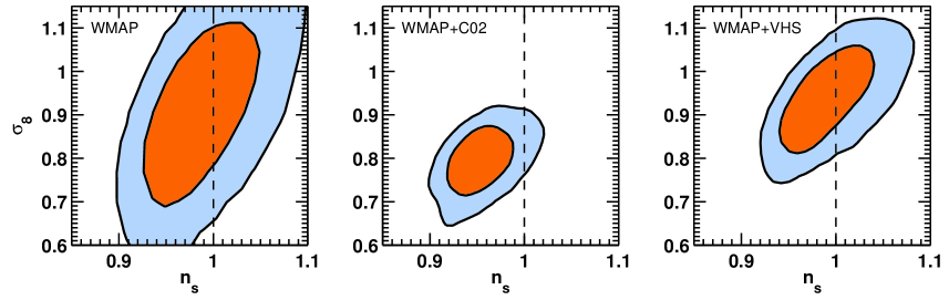
Figure 1: Joint $1$- and $2$-$\sigma$ likelihoods on $\sigma_{8}$ and n_s. In the left panel the constraints from WMAP only, the middle panel from WMAP combined with the Lyman-$\alpha$  power spectrum of C02, for a $\tau_{\rm eff}=0.349$. On the right the constraints from WMAP combined with VHS, for a $\tau_{\rm eff}(z=2.125)=0.17$ and $\tau_{\rm eff}(z=2.72)=0.305$. The dashed lines indicate the spectral index for a scale invariant ${\mbox{n${}_{\rm s}$}}=1$ primordial spectrum.

We extended the COSMOMC package (Lewis & Bridle 2002) to include the Lyman-$\alpha$ data as discussed in Section 2. As mentioned before the main uncertainty of the Lyman-$\alpha$ data is its relative calibration with respect to the underlying dark matter power spectrum. This is mainly influenced by the effective optical depth $\tau_{\rm eff}$, the normalization and slope of the temperature-density relation, $T_{0}$ and $\gamma$ and the other uncertainties described in section 2.2. We describe this uncertainty with an effective calibration amplitude $A$ and obtain for the log-likelihood

$$-\ln{\cal L}_{Ly\alpha}\propto\sum_{k}\frac{\left[A\,P_{\rm dat}(k)-P_{\rm th}(k)\right]^{2}}{\sigma_{P}^{2}}\,.$$ (3)

We introduce the calibration $A$ as an extra parameter into the Markov chain and multiply the likelihood with the prior

$$P_{\rm prior}\propto\exp\left[-\frac{1}{2}\frac{\left(A-{\bar{A}}\right)^{2}}{\sigma_{A}^{2}}\right]\,.$$ (4)

In order to obtain constraints on the cosmological parameters we will marginalize over the calibration parameter $A$. Note that this differs from the method described in Verde et al. (2003). As a standard prior on the mean we choose ${\bar{A}}=1$.

The cosmological parameters which are varied for the combined analysis are the physical baryon density ${\mbox{$\Omega_{\rm b}$}}\,h^{2}$, the physical dark matter density $\Omega_{\rm c}\,h^{2}$, the angular diameter distance to last scattering $\theta$, the optical depth $\tau$ due to instantaneous complete reionization, the amplitude A_s of primordial perturbations and as mentioned above the spectral index of scalar perturbations, either running or constant. Note that we restrict the analysis to a flat universe with a cosmological constant, where we neglect the contribution from neutrinos and tensor modes. We further restrict the analysis to optical depths $\tau<0.3$ as suggested by the WMAP team (Spergel et al. 2003, Verde et al. 2003). The amplitude of the matter fluctuations in a 8 Mpc$/h$ sphere, $\sigma_{8}$, is a derived quantity for this analysis.

We first discuss the results when we assume a constant spectral index n_s (${\mbox{n${}_{\rm run}$}}=0$).

In Figure 1 we show the joint likelihood for the scalar spectral index $n_{s}$ and $\sigma_{8}$. On the left is the result for WMAP only. Note that we only include the WMAP data set and not the extended CMB data set in order to concentrate on the constraints which are obtained by adding the Lyman-$\alpha$  forest. The WMAP data alone gives only very weak limits on the amplitude of the matter fluctuations and the spectral index. For a marginalized likelihood the spectral index is $n_{s}=0.990\pm 0.039$, consistent with a scale invariant power spectrum as found by the WMAP team and other authors. In the middle panel we show the result if we combine the WMAP data with Lyman-$\alpha$ data from C02 as compiled by Gnedin & Hamilton (2002). Note that we impose an uncertainty on the calibration of $\sigma_{A}=0.25$ if $A<1$ and $\sigma_{A}=0.29$ if $A>1$ (Verde et al. 2003). The spectral index differs now from a scale invariant $n_{s}=1$ primordial spectrum at the 2$\sigma$ level. The marginalized best fit value is $n_{s}=0.955\pm 0.023$. The right panel shows result for the WMAP data combined with the DM power spectrum as inferred by VHS. For this data we use a prior with $\sigma_{A}=0.29$ throughout, which is twice the uncertainty of the rms fluctuation amplitude as discussed in Section 2. As discussed in detail by VHS, the inferred amplitude is about 20% larger compared to that inferred by the C02 data with the lower effective optical depth. The spectral index is consistent with a scale invariant spectrum with $n_{s}=0.992\pm 0.032$. There is no significant evidence for a non-scale invariant spectrum in agreement with the simpler analysis in VHS which obtained ${\mbox{n${}_{\rm s}$}}=1.01\pm 0.02(\rm{stat.})\pm 0.06(\rm{syst.})$ and $\sigma_{8}=0.93\pm 0.03(\rm{stat.})\pm 0.09(\rm{syst.})$.

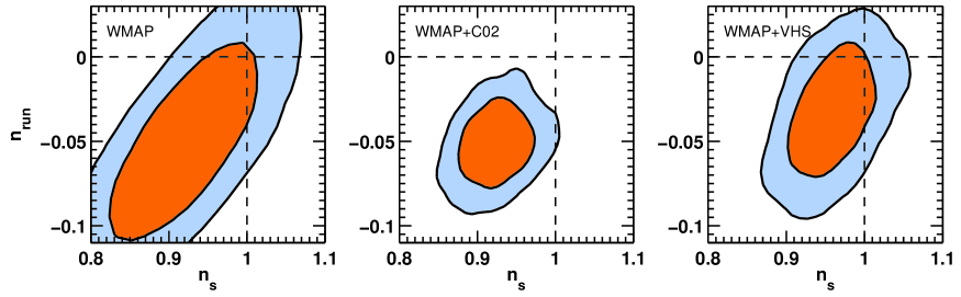
Figure 2: Joint $1$- and $2$-$\sigma$ likelihoods on n_run and n_s. In the left panel the constraints are from the WMAP only, the middle panel from WMAP combined with the Lyman-$\alpha$  power spectrum of C02, for a $\tau_{\rm eff}(z=2.72)=0.349$. On the right the constraints from WMAP combined with the results of VHS, for a $\tau_{\rm eff}(z=2.125)=0.17$ and $\tau_{\rm eff}(z=2.72)=0.305$. The dashed lines indicate a scale-invariant ${\mbox{n${}_{\rm s}$}}=1$ and ${\mbox{n${}_{\rm run}$}}=0$ primordial spectrum.

In Figure 3 we show the dependence of the $\sigma_{8}$ inferred from the combined analysis on the amplitude of the power spectrum inferred from the Lyman-$\alpha$ forest (parameterized as $A$, eq. 3). The dependence around the best fitting value is quite close to linearity ($\sigma^{2}_{8}\approx A)$. This plot was obtained with a prior on A given by eq. (3). The contours close at small and large values due to the constraints by the WMAP data alone. On the same axis we show explicitly the dependence on the effective optical depth (relative to the assumed best fitting value). The degeneracy of the inferred amplitude with the assumed effective optical depth already discussed by C02 and Seljak et al. (2003) is clearly seen. For the relation between amplitude A and effective optical depth we assumed $A\propto\tau_{\rm eff}^{-1.4}$ as found by VHS.

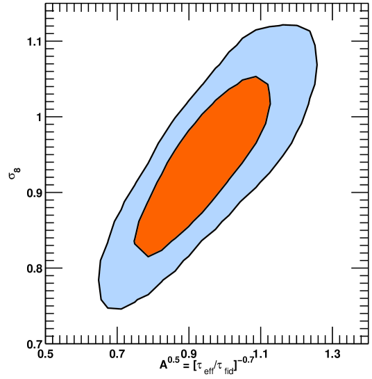
Figure 3: Joint $1$- and $2$-$\sigma$ likelihoods on $\sigma_{8}$ as a function of the amplitude of the power spectrum $A$ and of the effective optical depth.

We will now discuss the constraints which we obtain if we include a running spectral index. In Figure 2 we show the joint $1\sigma$ and $2\sigma$ likelihoods in the $n_{\rm run}$-$n_{s}$ plane marginalized over all other parameters. In the left panel we show the constraints from WMAP only. Again there is no significant evidence for a deviation from a simple scale invariant power spectrum, although the marginalized best fit values are ${\mbox{n${}_{\rm s}$}}=0.922\pm 0.062$ and ${\mbox{n${}_{\rm run}$}}=-0.050\pm 0.037$. In the middle we show the result from combining WMAP with the C02 data. The best fit values are $n_{s}=0.924\pm 0.030$ and ${\mbox{n${}_{\rm run}$}}=-0.052\pm 0.016$. This would rule out the most simple scale invariant power spectrum on the $3$-$\sigma$ level. This is consistent with the findings of the WMAP team but somewhat unusual for slow-roll inflationary models which require n_run to be of the order of $(|{\mbox{n${}_{\rm s}$}}-1|)^{2}$ (Kosowsky & Turner 1995; but see Dodelson & Stuart 2002). If we instead combine the VHS data with WMAP (right panel) the contours shift again towards a scale invariant spectrum with no running of the spectral index. The marginalized one dimensional errors are ${\mbox{n${}_{\rm s}$}}=0.959\pm 0.035$ and $n_{\rm run}=-0.033\pm 0.025$. This makes the difference to a simple scale invariant primordial power spectrum statistically insignificant.

Table 1: The marginalized results on cosmological parameters. The quoted values correspond to the peaks of the marginalized probability distributions. Errors are the 68% confidence limits.

	WMAP+C02 (power law)	WMAP+VHS (power law)	WMAP+C02 (running)	WMAP+VHS (running)
$\Omega_{\rm c}h^{2}$	$0.109\pm 0.010$	$0.124\pm 0.013$	$0.124\pm 0.013$	$0.132\pm 0.015$
$\Omega_{\rm b}h^{2}$	$0.022\pm 0.009$	$0.024\pm 0.001$	$0.022\pm 0.001$	$0.023\pm 0.001$
$h$	$0.721\pm 0.040$	$0.704\pm 0.047$	$0.683\pm 0.048$	$0.677\pm 0.047$
$\tau$	$0.115\pm 0.056$	$0.157\pm 0.068$	$0.192\pm 0.065$	$0.182\pm 0.069$
$\sigma_{8}$	$0.794\pm 0.052$	$0.936\pm 0.079$	$0.921\pm 0.071$	$0.978\pm 0.090$
ns	$0.955\pm 0.023$	$0.992\pm 0.032$	$0.924\pm 0.030$	$0.959\pm 0.036$
$n_{\rm{run}}$	-	-	$-0.052\pm 0.016$	$-0.033\pm 0.025$

In Table 1 we show the constraints on all the cosmological parameters for the combined WMAP and Lyman-$\alpha$ analysis with and without a running spectral index.

3.2 Constraining Slow-Roll Inflation

In order to obtain model independent constraints on inflation we concentrate on slow roll models. Since we are using a running of the spectral index of the scalar perturbations over a wide range in wavenumbers we use a second order extension of the standard slow-roll approximation (Liddle & Lyth 1993). This is described by the parameters (Martin & Schwarz 2000, Leach et al. 2002)

$$\epsilon_{1}\simeq\frac{M_{\rm Pl}^{2}}{2}\left(\frac{V^{\prime}}{V}\right)^{2}\;,$$ (5)

$$\epsilon_{2}\simeq 2{M_{\rm Pl}^{2}}\left[\left(\frac{V^{\prime}}{V}\right)^{2}-\frac{V^{{}^{\prime\prime}}}{V}\right]\;,$$ (6)

$$\epsilon_{2}\epsilon_{3}\simeq 2{M_{\rm Pl}^{4}}\left[\frac{V^{\prime\prime\prime}V^{\prime}}{V^{2}}-3\frac{V^{\prime\prime}}{V}\left(\frac{V^{\prime}}{V}\right)^{2}+2\left(\frac{V^{\prime}}{V}\right)^{4}\right]\;,$$ (7)

where primes denote derivatives with respect to the field and $M_{\rm Pl}=(8\pi G)^{-1/2}$ is the reduced Planck mass. Note that $\epsilon_{1},\,\epsilon_{2},\,\epsilon_{3}$ correspond to the conventional slow-roll parameters by $\epsilon_{1}=\epsilon_{V}$, $\epsilon_{2}=2\epsilon_{V}-2\eta_{V}$ and $\epsilon_{2}\epsilon_{3}=4\epsilon_{V}^{2}-6\epsilon_{V}\eta_{V}+2\xi_{V}$. If we calculate the spectrum of primordial perturbations in the inflaton field we can identify the slow-roll parameters with parameters of the power spectrum. In general inflation also predicts tensor fluctuations or gravitational waves. We neglect here the running of the tensor index which is given by $n_{\rm t}^{\rm run}=\epsilon_{1}\epsilon_{2}$. With the slow-roll conditions we obtain

$${\mbox{n${}_{\rm s}$}}-1 \approx -2\epsilon_{1}-\epsilon_{2}-2\epsilon_{1}^{2}-C\epsilon_{2}\epsilon_{3}\;,$$ (8)

$$r \approx 16\epsilon_{1}\,,$$ (9)

n_run $$\approx -\epsilon_{2}\epsilon_{3}\,,$$ (10)

with $C\approx 0.73$. We then obtain as a “consistency” relation between the scalar to tensor ratio $r$ and the tensor spectral index

$${\mbox{n${}_{\rm t}$}}=-\frac{r}{8}-\frac{r^{2}}{128}\;.$$ (11)

Note that this is only true if we neglect the running of the tensor spectral index. We will calculate the slow-roll quantities from the Markov chains generated in the parameters n_s, n_run and $r$. In this case we chose as the pivot scale $k_{0}=0.002\;{\rm Mpc}^{-1}$ (Peiris et al. 2003).

We perform a parameter analysis as described in Section 3.1 at this pivot scale with the addition of tensor modes with a free amplitude ratio $r<1$ and the constraint in equation (11).

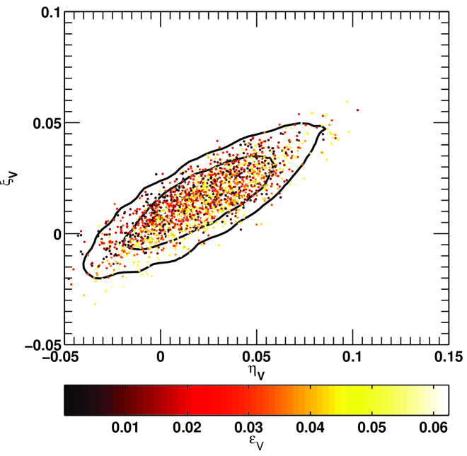
Figure 4: Joint likelihood in the $\eta_{V}$-$\xi_{V}$ plane, where the colour coding of the dots is scaled with $\epsilon_{V}$. The contours are the 68% and 95% confidence levels.

In Figure 4 we show the results of this analysis. The plot shows the results in the $\eta_{V}$-$\xi_{V}$ plane. The models are colour coded according to the third slow-roll parameter $\epsilon_{V}$. From equation (9) we see that $0<\epsilon_{V}<0.0625$, if we restrict the analysis to $r<1$. For most models of inflation there is a negligible contribution of gravitational waves to the perturbations, i.e. $r\sim\epsilon_{V}\approx 0$ (Liddle & Lyth 2000). In this case the likelihood contour in Figure 4 is restricted to the area depicted by the dark points, towards the lower left of the figure. $\eta_{V}$ and $\xi_{V}$ are thus relatively small, which according to equations (8) and (10) corresponds to a spectrum very close to scale invariant scalar fluctuations. This is consistent with our findings in Section 3.1. However, with the current data, models with a large tensor contribution are also valid, which correspond to the light coloured points in Figure 4, in the top right corner. The marginalized best fit values for the slow-roll parameters are $\epsilon_{V}=0.032\pm 0.018$, $\eta_{V}=0.020\pm 0.025$ and $\xi_{V}=0.015\pm 0.014$. The constraint on the tensor to scalar ratio is $r=0.499\pm 0.296$.

4 Conclusion

We have combined the linear dark matter power spectrum inferred from the Lyman-$\alpha$ forest with the 1st year WMAP data to obtain constraints on the rms fluctuation amplitude of matter fluctuations $\sigma_{8}$ and on the slope and shape parameter of the primordial density power spectrum n_s and n_run. We have restricted our analysis to spatially flat models with a low gravitational wave contribution to the CMB fluctuations. The WMAP data alone provides only weak constraints on $\sigma_{8}$, n_s and n_run. Adding the Lyman-$\alpha$ forest significantly tightens the constraints because of the resulting long lever arm which spans more than 3 orders of magnitude in wavenumber. The WMAP data combined with the DM power spectrum inferred by Croft et al. (2002) from their Lyman-$\alpha$ forest data requires a tilt (${\mbox{n${}_{\rm s}$}}<1$) and/or running of the spectral index (${\mbox{n${}_{\rm run}$}}<0$) to fit the data which is significant at the 3 $\sigma$ level. If we combine instead the WMAP data with the DM power spectrum inferred by VHS a smaller tilt and running of the spectral index are required which are not statistically significant. The best fit value for the rms fluctuation amplitude of matter fluctuations is $\sigma_{8}=0.94\pm 0.08$ and ${\mbox{n${}_{\rm s}$}}=0.99\pm 0.03$, in good agreement with the simpler analysis presented by VHS.

The difference of the analysis for the DM power spectrum of C02 and VHS is mainly due to the more appropriate smaller effective optical depth obtained from high resolution, high S/N QSO absorption spectra which was assumed in VHS. We further included tensor modes and put constrains on the slow roll parameters. At present the limits on $\epsilon_{V}$, $\xi_{V}$ and $\eta_{V}$ are not very tight, but future CMB missions such as Planck, together with better understanding of the systematic uncertainties of the Lyman-$\alpha$ forest data will improve the constraints.

References

- [] Bennett C. L., et al., 2003, ApJS, 148, 1
- [] Croft R. A. C., Weinberg D. H., Katz N., Hernquist L., 1998, ApJ, 495, 44
- [] Croft R. A. C., Weinberg D. H., Pettini M., Hernquist L., Katz N., 1999, ApJ, 520, 1
- [] Croft R. A. C., Weinberg D. H., Bolte M., Burles S.,Hernquist L., Katz N.,Kirkman D., Tytler D., 2002, ApJ, 581, 20 [C02]
- [] Dodelson S., Stewart E., 2002, Phys. Rev. D, 65, 101301
- [] Gnedin N. Y., Hamilton A. J. S., 2002, MNRAS, 334, 107
- [] Hannestad S., Hansen S.H., Villante F.L., Hamilton A.J.S., 2002, Astropart.Phys. 17, 375
- [] Hinshaw G. et al., 2003, ApJS, 148, 135
- [] Hui L., 1999, ApJ, 516, 519
- [] Hui L., Burles S., Seljak U., Rutledge R. E., Magnier E., Tytler D., 2001, ApJ, 552, 15
- [] Kim T.-S., Viel M., Haehnelt M.G., Carswell R.F., Cristiani S., 2004, MNRAS, 347, 355 (K04)
- [] Kinney W.H., Kolb E.W., Melchiorri A., Riotto A., 2004, Phys.Rev. D69, 103516
- [] Kogut A. et al., 2003, ApJS, 148, 161
- [] Kosowsky A., Turner S. M., 1995, Phys. Rev. D, 52, 1739
- [] Leach S.M., Liddle A.R., Martin, J., Schwarz, D.J., 2002, Phys. Rev., D66, 023515
- [] Leach S.M., Liddle A.R., 2003, Phys. Rev., D68, 123508
- [] Lewis A., Bridle S., 2002, Phys. Rev., D66, 103511
- [] Liddle A. R., Lyth D.H., 1993, Phys. Rep., 231, 1
- [] Liddle A. R., Lyth D.H., 2000, ”Cosmological Inflation And Large-Scale Structure”, Cambridge University Press ”
- [] Martin J., Schwarz D., 2000, Phys. Rev., D62, 103520
- [] McDonald P., Miralda-Escudé J., Rauch M., Sargent W.L., Barlow T.A., Cen R., Ostriker J.P., 2000, ApJ, 543, 1
- [] McDonald P., 2003, ApJ, 585, 34
- [] McDonald P. et al., 2004, astro-ph/0405013
- [] Page L. et al., 2003, ApJS, 148, 233
- [] Peiris H. et al., 2003, 148, 213
- [] Phillips J., Weinberg D. H, Croft R.A.C., Hernquist L., Katz N., Pettini M., 2001, 560, 15
- [] Ricotti M., Gnedin N., Shull M., 2000, ApJ, 534, 41
- [] Schaye J., Theuns T., Rauch M., Efstathiou G., Sargent W. L. W., 2000, MNRAS, 318, 817
- [] Seljak U., McDonald P., Makarov A., 2003, astro-ph/0302571
- [] Spergel D. N. et al. 2003, ApJS, 148, 175
- [] Tegmark M. et al., 2004, ApJ, 606, 702
- [] Verde L., et al. 2003, ApJS, 148, 195
- [] Viel M., Matarrese S., Theuns T., Munshi D., Wang Y., 2003, MNRAS, 340, L47
- [] Viel M., Haehnelt M.G., Springel V., 2004, MNRAS, 354, 684
- [] Zaldarriaga M., Hui L., Tegmark M., 2001, ApJ, 557, 519
- [] Zaldarriaga M., Scoccimarro R., Hui L., 2003, ApJ, 590, 1