The $N$-point correlation functions of the first-year Wilkinson Microwave Anisotropy Probe sky maps

Abstract

We compute the two-, three- and four-point correlation functions from the Wilkinson Microwave Anisotropy Probe (WMAP) first-year data, and compare these to a Monte Carlo ensemble of 5000 realizations, based on the best-fit WMAP running-index spectrum of Gaussian fluctuations. The analysis is carried out in three steps, covering small ($<72\arcmin$), intermediate ($<5^{\circ}$) and large scales (up to $180^{\circ}$). On the largest scales our results are consistent with the previously reported hemisphere power asymmetries: the northern ecliptic hemisphere is practically devoid of large scale fluctuations, while the southern hemisphere show relatively strong fluctuations. We also detect excess correlations in $W$-band difference maps as compared to the detailed noise simulations produced by the WMAP team, possibly indicative of unknown systematics. While unlikely to affect any temperature based results, this effect could potentially be important for the upcoming polarization data. On intermediate angular scales we find hints of a similar anisotropic distribution of power as seen on the very largest scales, but not to the same extent. In general the model is accepted on these scales. Finally, the same is also true on the smallest scales probed in this paper.

1. Introduction

In recent months, a large number of analyses focusing on non-Gaussianity in the Wilkinson Microwave Anisotropy Probe (WMAP; Bennett et al. 2003a) data have claimed significant detections of non-Gaussian features (Copi et al., 2004; de Oliveira-Costa et al., 2004; Eriksen et al., 2004a, b; Hansen et al., 2004a, b; Larson & Wandelt, 2004; McEwen et al., 2004; Park, 2004; Vielva et al., 2004). If any one of these detections can be shown to be of cosmological origin, currently accepted models based on Gaussianity and isotropy would have to be revised. Gaining proper understanding of their nature is therefore essential for further progress.

Sources of non-Gaussian (or anisotropic) signal may be categorized into three general classes. First, most non-cosmological foregrounds are highly non-Gaussian, and are all likely to introduce a non-Gaussian signal into the maps to some extent. In fact, unless some particular detection is explicitly demonstrated to be frequency-independent, it must usually be assumed to be foreground-induced. Second, systematics may introduce non-Gaussian signals into the data. An example of this is correlated noise, that results in stripes along the scanning path of the experiment. Finally, the most intriguing possibility is that the primordial density field itself could be non-Gaussian, e.g., through the existence of topological defects or non-equilibrium inflation.

In the current paper, we subject the WMAP data to an analysis based on real-space $N$-point correlation functions. While harmonic-space methods often are preferred over real-space methods for studying primordial fluctuations, real-space methods may have an advantage with respect to systematics and foregrounds, since such effects are usually localized in real space. It is therefore important to analyze the data in both spaces in order to highlight different features. For instance, by considering difference maps between independent differencing assemblies (abbreviated DA; see Hinshaw et al. [2003] for details on the terminology), that ideally should contain no CMB signal, we detect excess correlations in the data that are not accounted for in detailed simulations of the WMAP pipeline, and by partitioning the sky into small regions, we find hints of residual foregrounds near the galactic plane.

The algorithms used in this paper were developed by Eriksen et al. (2004c), and applied to the first-year WMAP data by Eriksen et al. (2004a). Other $N$-point correlation function analyses of the first-year WMAP data include those presented by Gaztañaga et al. (2003), Gaztañaga & Wagg (2003), and Land & Magueijo (2004).

2. Definitions

The statistics of interest in this paper are the $N$-point correlation functions (here restricted to two-, three- and four-point functions), and we measure these functions both for the observed data and for an ensemble of simulated realizations with controlled properties. A $\chi^{2}$ statistic is then employed to quantitatively measure the agreement between the data and the model.

An $N$-point correlation function is by definition the average product of $N$ temperatures, measured in a fixed relative orientation on the sky,

$$C_{N}(\theta_{1},\ldots,\theta_{2N-3})=\biggl{<}\Delta T(\hat{n}_{1})\cdots\Delta T(\hat{n}_{N})\biggr{>},$$ (1)

where the unit vectors $\hat{n}_{1},\ldots,\hat{n}_{N}$ span an $N$-point polygon on the sky. By assuming statistical isotropy, the $N$-point functions are only functions of the shape and size of the $N$-point polygon, and not on its particular position or orientation on the sky. Hence, the smallest number of parameters that uniquely determines the shape and size of the $N$-point polygon is $2N-3$.

The $N$-point correlation functions are estimated by simple product averages,

$$C_{N}(\theta_{1},\ldots,\theta_{2N-3})=\frac{\sum_{i}w_{1}^{i}\cdots w_{N}^{i}\cdot T_{1}^{i}\cdots T_{N}^{i}}{\sum_{i}w_{1}^{i}\cdots w_{N}^{i}},$$ (2)

where the sums are taken over all sets of $N$ pixels fulfilling the geometric requirements set by $\theta_{1},\ldots,\theta_{2N-3}$. The pixel weights, $w_{i}$, may be independently chosen for each pixel in order to reduce, e.g., noise or border effects. Here they represent masking, by being set to 1 for included pixels and to 0 for excluded pixels.

The main difficulty with computing $N$-point functions is their computational scaling. The number of independent pixel combinations scales as $\mathcal{O}(N_{\textrm{pix}}^{N})$, and for each combination of $N$ pixels, $2N-3$ angular distances must be computed to uniquely determine the properties of the corresponding polygon. Computing the full $N$-point function for $N>2$ and $N_{\textrm{pix}}\gtrsim 10^{5}$ is therefore computationally challenging.

However, it is not necessary to include all possible $N$-point configurations in order to produce interesting results. E.g., one may focus only on small angular scales, or on configurations with some special symmetry properties. By using the methods described by Eriksen et al. (2004c), the computational expense then becomes tractable, since no CPU time is spent on excluded configurations. In this paper several such subsets are computed, covering three distinct ranges of scales, namely small (up to $1\fdg 2$), intermediate (up to $5^{\circ}$) and large scales (the full range between $0^{\circ}$ and $180^{\circ}$).

2.1. The $\chi^{2}$ statistic

In this paper, a simple $\chi^{2}$ test is chosen to quantify the degree of agreement between the simulations and the observations, where $\chi^{2}$ as usual is defined by

$$\chi^{2}=\sum_{i,j=1}^{N_{\textrm{bin}}}(C_{N}(i)-\bigl{<}C_{N}(i)\bigr{>})M_{ij}^{-1}(C_{N}(j)-\bigl{<}C_{N}(j)\bigr{>}).$$ (3)

Here $C_{N}(i)$ is the $N$-point correlation function for configuration number $i$, $\bigl{<}C_{N}(i)\bigr{>}$ is the corresponding average from the Monte Carlo ensemble, and

$$M_{ij}=\frac{1}{N_{\textrm{sim}}}\sum_{k=1}^{N_{\textrm{sim}}}(C^{(k)}_{N}(i)-\bigl{<}C_{N}(i)\bigr{>})(C^{(k)}_{N}(j)-\bigl{<}C_{N}(j)\bigr{>})$$ (4)

is the covariance matrix.

This statistic is optimized for studying Gaussian distributed data. Unfortunately, the $N$-point correlation functions (and in particular even-ordered ones) are generally strongly non-Gaussian (and asymmetrically) distributed, and this leads to an uneven weighting of the two tails by the $\chi^{2}$ statistic. In order to remedy this weakness, the empirical distribution of each configuration is transformed by the relation (Eriksen et al., 2004a)

$$\frac{\textrm{Rank of observed map}}{\textrm{Total number of maps}+1}=\frac{1}{\sqrt{2\pi}}\int_{-\infty}^{s}e^{-\frac{1}{2}t^{2}}dt.$$ (5)

The numerator of the left hand side is the number of realizations with lower value than the current map, and the denominator is the total number of realizations plus 1. The addition of 1 is necessary to obtain symmetric values of $s$ around 0, and to avoid that the realization with the lowest value is assigned an infinite confidence level. Note that if the data were in fact Gaussian distributed, equation 5 is an identity operation in the limit of an infinite number of simulations. The $\chi^{2}$ statistic is then computed from the transformed data, rather than from the original correlation functions.

The quoted significance level is given in terms of the fraction of simulations with a lower $\chi^{2}$ value than the observed map. Thus, a value more extreme than either 0.025 or 0.975 indicates that the model is rejected at the $2\,\sigma$ level.

In order to eliminate any procedural difference between the simulations and the observed maps, we include the observed map itself in the estimation of the covariance matrix. While this should have no impact on the result if the covariance matrix is properly converged, it is a very useful safe-guard against such issues.

A singular value decomposition (SVD) is used to compute the inverse covariance matrix, and conservatively all modes with a condition number smaller than $10^{-6}$ are set to zero. However, this limit is only reached in the small-scale analysis, in which different neighboring configurations are very strongly correlated, and the covariance matrix converges more slowly than for the intermediate- and large-scale functions.

Finally, the four-point correlation function is treated differently than the two- and three-point functions, in that its power spectrum dependence is reduced by utilizing the following relationship: if a random field is Gaussian, then the ensemble average of the four-point function may be written in terms of the two-point function (see, e.g., Adler 1981),

$$\bigl{<}T_{1}T_{2}T_{3}T_{4}\bigr{>}= \bigl{<}T_{1}T_{2}\bigr{>}\bigl{<}T_{3}T_{4}\bigr{>}+\bigl{<}T_{1}T_{3}\bigr{>}\bigl{<}T_{2}T_{4}\bigr{>}$$ (6)

$$\quad+\bigl{<}T_{1}T_{4}\bigr{>}\bigl{<}T_{2}T_{3}\bigr{>}.$$ (7)

We therefore subtract the quantity on the right-hand side from the observed four-point function, to obtain a reduced four-point function. In what follows, all $\chi^{2}$ results for the four-point function refer to this reduced function.

3. Preparation of the data

The first-year WMAP data may be downloaded from LAMBDA. Most of the analyses described in the following sections are carried out for both the raw maps and the template-corrected versions (Bennett et al., 2003b).

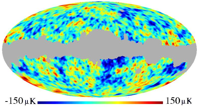
Figure 1.— The low-resolution co-added WMAP map is made by smoothing each of the eight cosmologically interesting bands to a common $\textrm{FWHM}=140^{\prime}$ Gaussian beam, and subsequently co-adding these using inverse-noise weights. Finally, best-fit monopole, dipole, and quadrupole moments were removed from the high-latitude region.

We define our model for the simulations as the sum of a CMB component and a noise component. The signal component is based on the best-fit WMAP power spectrum with a running index, including multipole components with $\ell=2,\ldots,1024$, filtered through the HEALPix (Górski, Hivon, & Wandelt 1999) pixel window functions and channel-dependent beam windows. While there is some controversy about the evidence for a running index, we have found that this spectrum provides a better fit to the data at the very low-$\ell$ range of the spectrum, and therefore a better fit in terms of $N$-point correlation functions that are sensitive to large-scale structures. However, this difference is only noticeable for the two-point function; the three-point and reduced four-point functions are only mildly dependent on the assumed power spectrum, thus our results should be independent thereof. Finally, the $a_{lm}$’s are assumed to be Gaussian.

The noise is assumed to be uncorrelated and Gaussian, with rms levels given for each pixel of each channel by the WMAP team (Bennett et al., 2003a). This noise is added pixel by pixel and channel by channel to the CMB signal realizations.

We study both individual frequency maps and a co-added version that includes all eight bands. The frequency maps are generated by straight averaging over bands using equal weights, whereas the co-added map is weighted with inverse noise variance weights (Hinshaw et al., 2003a).

The analysis is carried out in two steps: First we study the large-scale fluctuations on the full sky by degrading the maps from $N_{\textrm{side}}=512$ to $N_{\textrm{side}}=64$, $N_{\textrm{side}}$ being the HEALPix resolution parameter (Górski et al. 1999). We then study the small and intermediate scales by partitioning the full-resolution sky into disks of $10^{\circ}$ radius (in two different configurations), and compute the correlation functions on each disk separately. Full-sky functions for these scales are estimated by averaging over all disks.

The degradation process may be written on the following algorithmic form:

1. Compute the spherical harmonic components, $a_{\ell m}$ from the full resolution $N_{\textrm{side}}=512$ map.

2. Deconvolve with the original WMAP beam and pixel windows (i.e., multiplication in harmonic space).

3. Convolve with a $140\arcmin$ FWHM Gaussian beam and $N_{\textrm{side}}=64$ pixel windows.

4. Compute the $N_{\textrm{side}}=64$ map using the filtered $a_{\ell m}$’s.

This process is carried out for each channel separately before any co-addition is done. The downgraded, co-added WMAP map is shown in Figure 1.

Since all structures in the high-resolution maps are smoothed out in the degrading process, the foreground exclusion mask must also be extended correspondingly. This is done by setting all excluded pixels in the original mask to 0 and all included pixels to 1, then convolving this map with a Gaussian beam of the desired FWHM, and finally excluding all pixels with a value smaller than 0.99 in the smoothed mask.

This degraded mask will only be used on smoothed, low-resolution maps, and the Kp0 mask is therefore used with point sources not excluded as our base mask. This could in principle introduce a non-Gaussian signal into our maps, but in practice point sources contribute negligible power at scales larger than a few degrees (Hinshaw et al., 2003a).

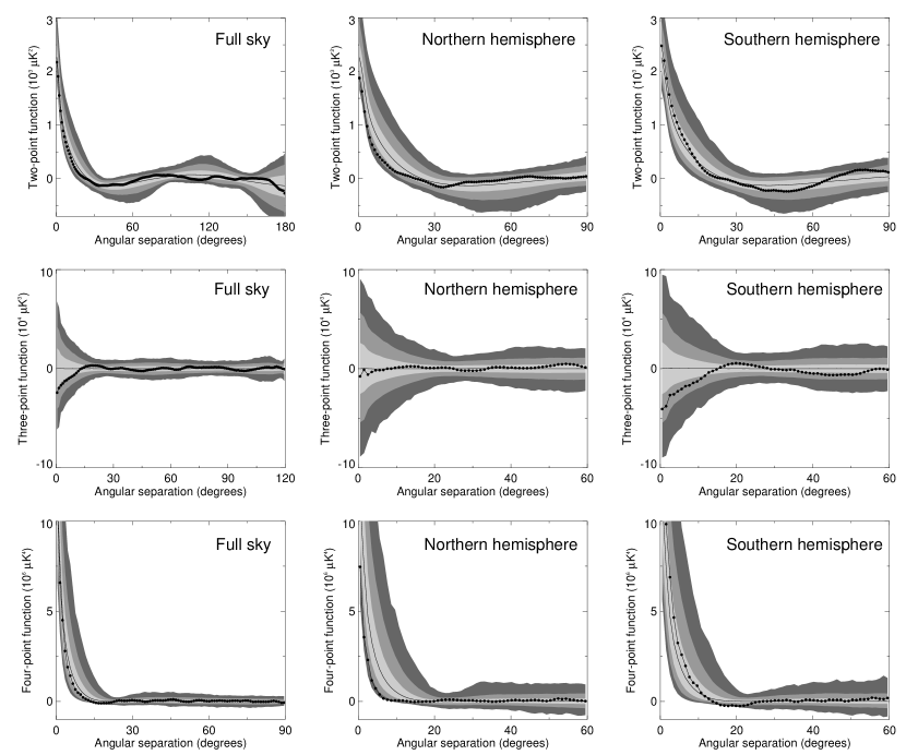
Figure 2.— The large-scale, low-resolution correlation functions computed from from the co-added WMAP map. The solid dots show the results from the observed data, the solid line and the gray bands show the median and the 1, 2, and $3\,\sigma$ confidence regions, respectively, computed from 5000 simulations. The full-sky, northern, and southern galactic hemisphere results are plotted in left, middle, and right columns, while rows show the two-point, the equilateral three-point, and the rhombic four-point functions. Note in particular the extremely featureless correlation functions computed on the northern hemisphere, indicating little large-scale structure in this region. Similar plots for the ecliptic hemispheres are shown by Eriksen et al. (2004a).

Finally, for the low-resolution analysis, we remove the monopole, dipole, and quadrupole modes from each map separately, with parameters computed from the high-latitude regions of the sky only (defined by the extended Kp0 mask). The reason for removing the quadrupole is that this particular mode may have an anomalously low value (Bennett et al., 2003a), but is certainly contaminated by residual foregrounds after template subtraction (Slosar & Seljak, 2004; Hansen et al., 2004b; Eriksen et al., 2004d). Since real-space correlation function are inherently more sensitive to the low-$\ell$ modes, this well-known effect could mask other interesting features.

In the case of the small- and intermediate-scale analyses, we estimate the correlation functions on independent disks of $10^{\circ}$ radius. In order to reduce the correlation between neighboring disks, we therefore choose to remove all multipoles with $0\leq\ell\leq 18$, by generalizing the usual method of removing the low-$\ell$ components to higher multipoles.

4. Large-scale analysis

The first analysis focuses on the very largest scales, by computing the $N$-point correlation functions from degraded maps, as described above. The functions are uniformly binned with $1^{\circ}$ bin size, and the two-point function is computed over the full range between 0 and $180^{\circ}$. For the higher-order functions we follow Eriksen et al. (2002) and compute the pseudo-collapsed and the equilateral three-point functions, and the 1+3-point and the rhombic four-point functions.

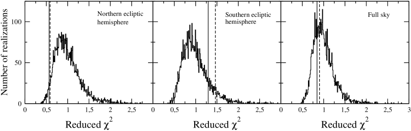
Figure 3.— Distributions of the $\chi^{2}$ values computed from the ensemble for the full sky three-point function; the plots show the results for the northern ecliptic hemisphere (left), the southern ecliptic hemisphere (middle), and the full sky (right). The value corresponding to the foreground corrected co-added map is marked with a solid line, while the raw co-added map is denoted with a dashed line.

The definition of “pseudo-collapsed” is slightly modified compared to the one described by Eriksen et al. (2002). In this paper “pseudo-collapsed” indicates that the length of the collapsed edge falls within the second bin, and not that only neighboring pixels are included (Gaztañaga et al., 2003; Eriksen et al., 2004a). This modification eliminates the need for treating each configuration as a special case, and is thus purely implementation-ally motivated.

The results from these measurements are shown in Figure 2 for the co-added map, for a few selected functions. A complete summary of the large-scale measurements are given in Table 1 for both individual channels and for the co-added map, and for two different masks.

Considering first the full-sky two-point function, we see that this function demonstrates an almost complete lack of structure above $60^{\circ}$, and its overall shape is very flat as pointed out by several authors (e.g., Bennett et al. 2003a). However, here it is important to remember that the quadrupole was removed prior to the computation of the correlation functions, and therefore the two-point function does not appear quite as anomalous as that seen in many other plots.

Table 1Large scale $N$-point correlation function $\chi^{2}$ and $S$-statistic results

	$Q$-band		$V$-band		$W$-band		Co-added
Region	Kp0	$|b|>30^{\circ}$	Kp0	$|b|>30^{\circ}$	Kp0	$|b|>30^{\circ}$	Kp0	$|b|>30^{\circ}$
Two-point function; $\chi^{2}$ statistic
Full sky	0.725	0.558	0.491	0.606	0.519	0.429	0.574	0.451
Northern galactic	0.495	0.605	0.721	0.732	0.682	0.574	0.772	0.578
Southern galactic	0.903	0.861	0.792	0.865	0.740	0.629	0.865	0.803
Northern ecliptic	0.439	0.508	0.608	0.582	0.218	0.536	0.538	0.469
Southern ecliptic	0.272	0.729	0.215	0.676	0.125	0.572	0.216	0.598
Two-point function; $S$-statistic results
Full sky	0.094	0.102	0.084	0.121	0.068	0.131	0.085	0.107
Northern galactic	0.026	0.439	0.019	0.379	0.036	0.417	0.022	0.419
Southern galactic	0.739	0.433	0.776	0.555	0.726	0.567	0.749	0.488
Ratio of $S$-values	0.033	0.239	0.025	0.168	0.034	0.203	0.029	0.214
Northern ecliptic	0.016	0.015	0.017	0.012	0.012	0.013	0.015	0.014
Southern ecliptic	0.745	0.693	0.791	0.784	0.743	0.794	0.759	0.735
Ratio of $S$-values	0.045	0.075	0.038	0.052	0.048	0.050	0.044	0.063
Three-point function; $\chi^{2}$ statistic
Full sky	0.314	0.711	0.267	0.636	0.154	0.616	0.284	0.641
Northern galactic	0.041	0.051	0.036	0.050	0.034	0.061	0.031	0.060
Southern galactic	0.825	0.796	0.819	0.847	0.819	0.774	0.822	0.821
Ratio of $\chi^{2}$’s	0.030	0.046	0.027	0.033	0.027	0.057	0.026	0.044
Northern ecliptic	0.047	0.046	0.023	0.033	0.014	0.038	0.034	0.041
Southern ecliptic	0.831	0.792	0.861	0.820	0.871	0.829	0.840	0.793
Ratio of $\chi^{2}$’s	0.031	0.040	0.014	0.031	0.012	0.031	0.023	0.039
Four-point function; $\chi^{2}$ statistic
Full sky	0.484	0.518	0.491	0.480	0.474	0.472	0.468	0.508
Northern galactic	0.089	0.073	0.069	0.053	0.086	0.051	0.077	0.061
Southern galactic	0.884	0.920	0.905	0.930	0.878	0.914	0.888	0.923
Ratio of $\chi^{2}$’s	0.030	0.022	0.020	0.014	0.031	0.017	0.025	0.018
Northern ecliptic	0.070	0.020	0.054	0.010	0.050	0.012	0.058	0.014
Southern ecliptic	0.852	0.927	0.873	0.942	0.846	0.931	0.857	0.932
Ratio of $\chi^{2}$’s	0.030	0.004	0.021	0.001	0.025	0.002	0.025	0.002

Note. — Results from $\chi^{2}$ tests of the large-scale correlation functions. The numbers indicate the fraction of simulations with a $\chi^{2}$ value lower than for the respective WMAP map.

Next, the full-sky three-point function shows similar tendencies, as it lies inside the $1\,\sigma$ confidence region almost over the full range of scales. Finally, the four-point function is quite low at small angles, and very close to zero at large angles. Thus, all three full-sky correlation functions point toward the same conclusion – there is little large-scale power in the WMAP data.

Several analyses have presented evidence for a significant asymmetry between the northern and southern ecliptic (and galactic) hemispheres (Eriksen et al., 2004a, b; Hansen et al., 2004a, b; Park, 2004), and therefore we choose to estimate the various functions from these regions separately. Similar patterns are indeed found also in these cases: the northern hemisphere correlation functions all show a striking lack of fluctuations, whereas the southern hemisphere functions show good agreement with the confidence bands computed from the Gaussian simulations. This difference translates into a clear difference of $\chi^{2}$ numbers, as seen in Table 1. The northern hemisphere results for the higher-order functions all lie in the bottom few percent range, while the corresponding numbers for the southern hemisphere are generally higher than 80%.

The $\chi^{2}$ statistic may actually serve as a general measure of the overall fluctuation level of the higher-order functions, since they both have vanishing mean (we use the reduced, not the complete, four-point function in these analyses; for the same reason, this does not work for the two-point function). One possible statistic for the degree of power asymmetry between two complimentary hemisphere is therefore simply the ratio of the two individual $\chi^{2}$’s. This quantity is computed for both the simulations and the observed data, and the fraction of simulations with a smaller ratio is listed in the third row of each section in Table 1.

We see that this ratio is extreme at the few percent level for the three-point function, and at less than one percent for the four-point function, for the ecliptic hemispheres. Further, it is not particularly sensitive to frequency or galactic cut. In fact, the numbers are slightly stronger for the conservative $|b|>30^{\circ}$ mask than for the Kp0 mask in four-point function case. Both these results argue strongly against a foreground based explanation.

In order to quantify the two-point function asymmetry, we adopt a slightly modified version of the $S$-statistic, as defined by Spergel et al. (2003)

$$S=\int[C_{2}(\theta)]^{2}\textrm{d}\cos\theta.$$ (8)

Note that we choose to include the full range of available angles, while Spergel et al. (2003) chose to exclude angles smaller than $60^{\circ}$. Excluding the smaller angles does increase the nominal significance of this statistic when applied to the WMAP data, but it also makes the interpretation of the final results less clear, since the cut-off scale is arbitrarily chosen.

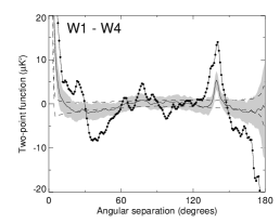
Figure 4.— Results from the difference map analysis. The solid dots show the results computed from the observed maps, while the solid line and the gray bands show the median and the $1\,\sigma$ confidence region, respectively, computed from the 110 simulations produced by the WMAP team, including all known systematic effects. The dashed lines indicate the $1\,\sigma$ confidence region assuming uncorrelated noise, modulated by $N_{\textrm{obs}}(p)$ only.

In general, the $S$-statistic has similar properties to a $\chi^{2}$ statistic that only includes diagonal terms, but it has a distinct advantage over the latter in the case of the two-point function: while both power deficits and excesses lead to a large $\chi^{2}$ (rendering this statistic useless for probing asymmetry), the opposite is true for the $S$-statistic. Power deficit yields a low $S$-value, while power excess yields a high $S$-value. In other words, this statistic may serve the same purpose for the two-point function as the $\chi^{2}$ statistic does for the higher-order functions.

The results from this analysis are shown in the second section of Table 1. Overall, they are consistent with the $\chi^{2}$-based three- and four-point function results, with the single exception of the galactic $|b|>30^{\circ}$ measurements, which do not show any signs of asymmetry. However, in this case the two-point function is quite poorly constrained at the largest angles because of the limited sky coverage, and sample variance dominates the statistic.

In Figure 3 the histograms of the $\chi^{2}$ values for the co-added simulated ensemble are plotted together with the observed WMAP values (both for the foreground-corrected and the raw maps). In this Figure it is well worth noting the effect of foregrounds, namely that the $\chi^{2}$ increases if foregrounds are present. This is both an intuitive and an important result: it is intuitive because the $\chi^{2}$ statistic basically measures the amount of deviations from the average function, and for a function with vanishing mean such as the three-point function, it therefore quantifies the overall level of fluctuations. By adding a statistically independent component to the maps (residual foregrounds in our setting), more fluctuations are introduced into the three-point function. This observation is therefore also important, since it implies that residual foregrounds are unlikely to explain the northern hemisphere anomaly – sub-optimal foreground templates would introduce large-scale fluctuations, rather than suppress them. This also suggests that one could use the $\chi^{2}$ statistic as defined above to fit for the template amplitudes, a possibility that will be explored further in a future publication.

All in all, the results presented in this section seem to disfavor a foreground-based explanation for the large-scale power asymmetry. The variation from band to band is very small indeed, and similar signs of asymmetry can be seen in any one of the frequencies. Further, there is no clear dependence on the particular sky cut.

4.1. Analysis of difference maps

Next, we study the noise properties of the WMAP data. Specifically, the two-point correlation functions are computed from all possible difference maps within each frequency channel, and we compare these to the functions computed from corresponding correlated noise maps produced by the WMAP team. All data have been processed in the same way as for the large-scale analysis; the maps are downgraded to a common resolution of $140^{\prime}$, then the difference maps are formed, and finally, the best-fit monopole, dipole and quadrupole moments are removed from the extended Kp0 region.

In Figure 4 the results from this analysis are shown, comparing the WMAP data (solid dots) to the simulations, that includes all known systematics. The gray bands indicate the $1\,\sigma$ confidence bands computed from the 110 available simulations, and the dashed lines show the $1\,\sigma$ regions assuming uncorrelated (but inhomogeneous) white noise, computed from 1000 simulations.

In particular two features stand out in these plots: First, there is a strong peak at $\theta_{\textrm{h}}=141^{\circ}$, the effective horn separation angle of the WMAP satellite. Second, there is a clear rise toward high values at small angles, which is a real-space manifestation of correlated noise. Of course, neither of these effects are unexpected, since they are also present in the simulations, and they are both discussed at some length by Hinshaw et al. (2003b).

However, there are a few surprises to be found in the $W$-band plots. Specifically, a very strong signal may be seen in the $W$1–$W$4 map. To the extent that the confidence regions can be approximated by Gaussians, we see that the peak at $\theta_{\textrm{h}}$ extends to more than $4\,\sigma$ compared to the simulations, and the overall fluctuation levels are clearly stronger than what is seen in the simulations. A similar pattern is also seen in the $W$1–$W$2 map, but with a slightly smaller amplitude.

Comparing the confidence regions estimated from correlated and white noise simulations, we see that the main difference is more large-scale curvature in the correlated noise bands. This is consistent with the power spectrum view, where correlated noise is found to have the strongest impact at low $\ell$’s. This again translates into a two-point function with a shape resembling that of the signal-dominated functions shown in Figure 2. This effect is particularly evident in the maps which involve the W4 differencing assembly, which is known to have a significantly higher knee frequency than the other DA’s (Jarosik et al., 2003).

We now quantify the agreement between the observations and the model by means of a $\chi^{2}$ statistic, but we do not attempt to include the correlation structure in this case because of the limited number of simulations. Rather, we define a simplified statistic on the following form,

$$\chi^{2}_{\textrm{diag}}=\sum_{i=1}^{N_{\textrm{bin}}}\frac{\left(C_{2}(i)-\bigl{<}C_{2}(i)\bigr{>}\right)^{2}}{\sigma^{2}(i)}.$$ (9)

Here $N_{\textrm{bin}}$ is the number of bins in the correlation function, and $\bigl{<}C_{2}(i)\bigr{>}$ and $\sigma^{2}(i)$ are the average and variance, respectively, of bin number $i$ computed from the simulations. Unsurprisingly, this statistic strongly rejects the model for the $W$1–$W$2 and $W$1–$W$4 combinations, as none of the 110 simulations have a higher $\chi^{2}_{\textrm{diag}}$ value than the observation, or even close to it. For the remaining six combinations, the ratios of simulations with a lower $\chi_{\textrm{diag}}^{2}$ all lie comfortably in the range between 0.28 and 0.94.

It is difficult to make firm conclusions about the origin of these structures based on this simple analysis alone, but it is evident that the noise simulations do not fully capture the nature of the data. On the other hand, it is also very unlikely that this effect has any significant impact on the cosmological results from the first-year WMAP data release, given its relatively small amplitude. It may be important with respect to the second-year polarization data.

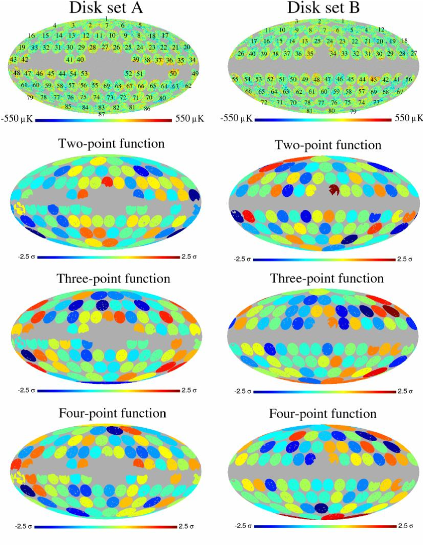
Figure 5.— Results from the intermediate scale correlation function analysis. The top panels show the layout of each disk set, and the other three rows show the $\chi^{2}$ results. The colors indicate the confidence level at which the disk is accepted, computed according to equation 5. Thus, dark blue indicates a very low $\chi^{2}$ value, green a value around the median, and dark red a very high $\chi^{2}$ value.

A similar detection was reported by Fosalba & Szapudi (2004). They found that the noise contribution in the WMAP data may have been underestimated by 8–15% in the original analysis. However, it is difficult to establish a direct connection between these results, considering that their results are most significant at high $\ell$’s, while our analysis is explicitly restricted to low $\ell$’s.

5. Small- and intermediate-scale analysis

In order to probe smaller scales, subsets of the $N$-point functions are now from the full-resolution co-added map. This analysis is facilitated by partitioning the sky into non-overlapping disks of $10^{\circ}$ radius, each including between 15 000 and 25 000 pixels (the number varies because of the Kp2 mask). Two different sets of disks (denoted A and B) are used in the following analysis, their union covers a total of 81% of the sky, and about 60% each. The two sets contain respectively 87 and 81 disks.

The reasons for dividing the sky into patches are two-fold: First, the computational cost soon becomes difficult to handle for data sets with more than about 150 000 pixels. Since the algorithms scale as a relatively high power of $N_{\textrm{pix}}$, it is much cheaper to divide the full region into patches. Second, and equally important, we want to be able to localize interesting effects in pixel space. In particular, we seek to study the effects discussed in §4 further, and one convenient way of doing this is by analyzing the sky in patches. A similar analysis was carried out by Hansen et al. (2004b), using a power spectrum based statistic.

The disk sets are created as follows: In each set, the disks are laid out on rings of constant latitude, with as many disks on each ring as there is space for without overlap (the polar rings of set B are exceptions to this rule), and random initial longitude. Then the WMAP Kp2 mask is applied and we keep only those “disks” (at this point some have a rather peculiar geometry) with more than 15 000 accepted pixels. The reason for preferring the more liberal Kp2 mask over Kp0 is that we also want to study the effect of foregrounds in this analysis.

The defining difference between set A and B is given by the latitudes on which the disks are centered. In set A, the disks are laid out on latitudes given by $\theta=k\cdot 20^{\circ}$, $k=0,\ldots,9$, while the disks in set B are centered on $\theta=(k+1/2)\cdot 20^{\circ}$, $k=0,\ldots,8$. This difference implies that set A has two rings of disks that touches the galactic plane, while the center ring of disk set B is completely discarded. It is therefore reasonable to assume that disk set A is more affected by foregrounds than disk set B, as will be confirmed later. The two disk sets are shown in the two top panels of Figure 5, superimposed on the co-added WMAP map.

5.1. Intermediate-scale analysis

First, we consider the $N$-point correlation functions on intermediate scales, here defined as scales smaller than 5–$10^{\circ}$. Each function is binned with $7\farcm 2$ bin size, and the two-point function is computed up to $10^{\circ}$, for a total of 83 bins. The three-point function is computed over all isosceles triangles for which the baseline is the longest edge, but no longer than $5^{\circ}$. Note that this set includes the equilateral triangle and three points on a line as special cases. Finally, the four-point function is computed over the same set of configurations, but with a fourth point added by reflecting the third point about the baseline. The total number of independent configurations is about 460. Note that since there are many more isosceles triangles with $5^{\circ}$ baseline than with $1^{\circ}$, the vast majority of these configurations span scales from $3^{\circ}$ to $5^{\circ}$. Consequently, the following $\chi^{2}$ analysis is dominated by intermediate scales rather than small scales, even though a few small-scale configurations are included.

The results from this intermediate scale analysis are plotted in Figure 5, where the colors indicate the confidence level at which each disk is accepted, as computed by equation 5. However, extreme limits of $-2.5\,\sigma$ and $2.5\,\sigma$ are enforced, because we only have a limited number of simulations available. Here it is worth recalling that we removed all power with $\ell\leq 18$ from the maps, and neighboring disks are therefore nearly uncorrelated. Distributions of the confidence level distributions are shown in Figure 6.

We see that the two-point function is to a very good approximation accepted by the $\chi^{2}$ test. There are no visibly connected patches of similar values, and the distribution of confidence values appears to be typical compared to the simulations. The three-point functions are more suspicious, especially when considering the pattern seen in disk set B. In this case, two large, connected patches of low $\chi^{2}$ values are visible on the northern hemisphere, while the south-east quadrant appears to have quite large $\chi^{2}$ values. In other words, the asymmetry pattern found in the large-scale functions is apparent even in this plot. For disk set A, these features are less clear, but still consistent with disk set B; the northern hemisphere on average have quite low $\chi^{2}$ values (or little fluctuations), while the south-east quadrant has quite high $\chi^{2}$ values. This is particularly evident if one disregards all disks touching (i.e., are partially cut by) the galactic plane, they are more likely to be affected by residue foreground contamination.

The four-point functions are less decisive, and the general agreement with the Gaussian model seems to be quite good. No particular features are seen in these cases.

We now estimate the full sky correlation functions by averaging over all the individual disk correlation functions, weighting each sub-function by the number of pixel combinations, $N_{\textrm{c}}$,

$$C_{N}^{\textrm{full sky}}(i)\approx\frac{\sum_{j=1}^{N_{\textrm{disks}}}N_{\textrm{c}}^{j}(i)\,C_{N}^{j}(i)}{\sum_{j=1}^{N_{\textrm{disks}}}N_{\textrm{c}}^{j}(i)}.$$ (10)

Here $C_{N}$ is the full-sky $N$-point correlation function, $C_{N}^{j}$ is the $j$’th disk correlation function, and $i$ represents the geometric configuration under consideration.

This function is computed from each disk set individually and over the union of the two sets. While the latter function obviously has the advantage of larger sky coverage, it also weights configurations that are completely contained in the intersection of two disks twice. On the other hand, the number of such common configurations is fairly small, at least in this intermediate-scale analysis.

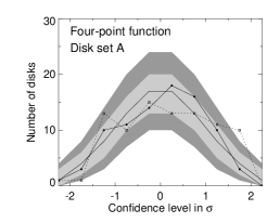
Figure 6.— Distributions (histograms) of the intermediate scale disk confidence levels. The top row shows the results for disk set A, the bottom for disk set B. The columns show, left to right, the two-, three-, and four-point function results. The gray bands indicate 1 and $2\,\sigma$ confidence regions, computed from 5000 simulations. The solid line indicates the results from the foreground corrected map, and the dotted line shows the results from the original co-added map.

In Figure 7 the full-sky, intermediate-scale two-point, equilateral three-point and rhombic four-point functions are plotted, as computed from equation 10. The corresponding $\chi^{2}$ results are shown in Table 2. We see that the agreement between observations and simulations is in all cases very good, both in terms of overall shape and amount of small-scale fluctuations. Note, however, that these figures only show a small subset of the configurations included in the full analysis; while there are 41 three-point configurations with a base line of $5^{\circ}$, there are only two with a $10^{\prime}$ base line. Thus, the right hand sides of the three- and four-point function plots are weighted much more strongly than the left hand side in the $\chi^{2}$ analysis. Generally speaking, visualizing higher-order functions is difficult because of their high dimensionality.

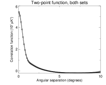
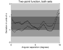
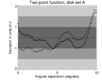
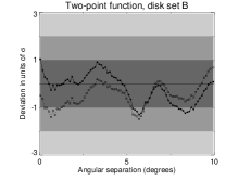
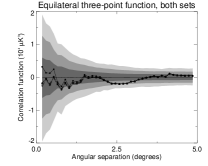
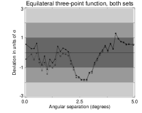
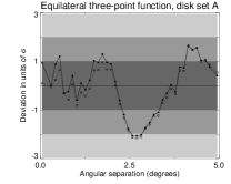
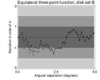
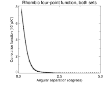
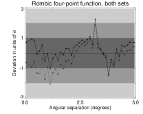
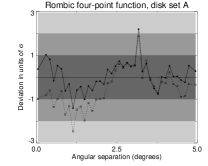
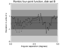
Figure 7.— The full-sky intermediate-scale correlation functions. The left-hand column shows the functions directly as measured from the union of the two disk sets, while the normalized functions (see equation 5) are shown in the other three columns. The gray bands indicate 1, 2, and $3\,\sigma$ bands, as computed from simulations. The dotted line corresponds to the foreground corrected map and the solid line to the uncorrected map.

The results from the corresponding $\chi^{2}$ analysis are shown in Table 2. Here we see that the results for the foreground corrected map all lie comfortably between 0.05 and 0.95, and no sign of discrepancy is found. For the raw maps, the $\chi^{2}$ numbers are generally somewhat high, but not disconcertingly so. The agreement with the assumed model on intermediate scales appears to be satisfactory on intermediate scales, as far as $N$-point correlation functions are concerned.

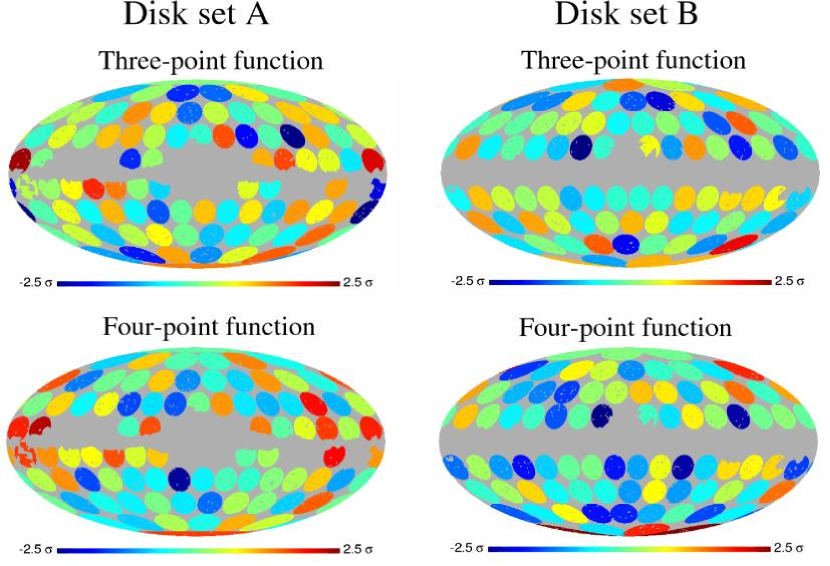
Figure 8.— Results from the small-scale correlation function analysis. The elements have the same meaning as in figure 5. Note the high $\chi^{2}$ values around the galactic plane in disk set A.

A similar analysis, including disks in the galactic or ecliptic hemispheres only, was also performed, but it did not find any clear discrepancy in either case. Thus, the asymmetric pattern seen in Figure 5 in the three-point function in set B does not correspond directly to a dipole type distribution. Of course, we could subdivide the sky further according to the observed patterns, but this would strongly dilute the final probabilities, since we then define our test a-posteriori. All in all, the intermediate scale correlation functions accepts the model, although hints of hemisphere asymmetry may be seen by eye in the three-point function.

5.2. Small-scale analysis

The analysis from the previous section is now repeated, but this time including all three-point configurations with a longest edge shorter than or equal to $72^{\prime}$ (about 220 different configurations), and twice as many four-point configurations. The four-point configurations are defined in terms of the three-point configurations, by letting the fourth point either be mirrored or rotated about the base line, that once again is defined to be the longest edge of the triangle.

The results from this disk-based analysis are shown in Figure 8, and distributions of the corresponding $\chi^{2}$ values are plotted in Figure 9. By eye, the three-point function results in Figure 8 appear to be in quite good agreement with the model, and no clear anomalies stand out. This impression is confirmed both by the full-sky $\chi^{2}$ numbers, as well as by the plots showing the disk $\chi^{2}$ distributions, except for the fact that there are quite a large number of disks in the 1–$1.5\,\sigma$ range in disk set B.

Figure 9.— Distributions (histograms) of the small scale disk confidence levels. The top row shows the results for disk set A, the bottom for disk set B. The columns show the three- and four-point function results, respectively. Gray bands indicate 1 and $2\,\sigma$ confidence regions, computed from 5000 simulations, the solid lines indicate the results from the foreground corrected map, and the dotted lines show the results from the raw co-added map.

However, the four-point function plot for disk set A shows a more interesting effect; at least 7 out of the 21 disks touching the galactic sky cut in disk set A have a fairly high $\chi^{2}$ value, and there are no disks with low $\chi^{2}$ values. This is most likely an indication of residual foregrounds near the galactic plane, a conclusion which becomes even more plausible when studying figure 11 in the paper by Bennett et al. (2003b). In these plots, clear residuals are seen outside the Kp2 mask, particularly in the $Q$-band map.

Table 2Intermediate scale $\chi^{2}$ results

Correlation function	Both sets	Disk set A	Disk set B
No foreground correction
Two-point	0.829	0.322	0.944
Three-point function	0.955	0.805	0.981
Four-point function	0.941	0.917	0.722
Foreground correction by external templates
Two-point function	0.756	0.189	0.901
Three-point function	0.816	0.527	0.938
Four-point function	0.683	0.674	0.330

Note. — Results from the intermediate scale full-sky $\chi^{2}$ tests. The numbers indicate the fraction of simulated realizations with $\chi^{2}$ value lower than that for the co-added WMAP map. The upper half shows the results before correcting for foregrounds, and the lower half shows the results after applying foreground corrections.

Table 3Small scale $\chi^{2}$ results

	Both sets	Disk set A	Disk set B
No foreground correction
Three-point function	0.725	0.600	0.554
Four-point function	0.325	0.507	0.360
Foreground correction by external templates
Three-point function	0.330	0.084	0.214
Four-point function	0.177	0.639	0.317

Note. — Results from the small scale full-sky $\chi^{2}$ tests. The numbers indicate the fraction of simulated realizations with $\chi^{2}$ value lower than that for the co-added WMAP map. The upper half shows the results before correcting for foregrounds, and the lower half shows the results after applying foreground corrections.

We may quantify the significance of this effect by computing a new disk-averaged correlation function. This time we include only those 21 disks in the two near-galactic rows (A34–54), and the corresponding results are shown in Table 4 for both intermediate and small scales.

The four-point function results have a combined significance at $2\,\sigma$ for the intermediate scales, and almost $3\,\sigma$ for the small scales. In fact, for the small scales even the three-point function has a $\chi^{2}$ value at the $2\,\sigma$ level. From these considerations, it seems likely that the simple foreground correction method by templates discussed by Bennett et al. (2003b) leaves significant residuals near the galactic plane. Indeed, this should not be surprising since the input synchrotron and free-free templates do not contain power on the small angular scales probed by the $Q$-, $V$-, and $W$-band maps, and the template fitting method itself does not admit spectral variations on the sky, while it is likely that such variations are seen close to the galactic plane.

We also compute the full-sky, disk-averaged correlation function for the small-scale functions, and the results from this $\chi^{2}$ analysis are shown in Table 3. Here we see that the model is comfortably accepted on these scales, and the effect of the foreground residuals discussed above is diluted by the additional sky coverage.

Table 4Galactic plane $\chi^{2}$ results

Scales	Two-point	Three-point	Four-point
Intermediate	0.533	0.826	0.975
Small	$\cdots$	0.975	0.998

Note. — Results from $\chi^{2}$ tests of the correlation functions computed over the disks near the galactic plane (disks A34-54).

Finally, we make one connection to a previously reported detection of non-Gaussianity (Vielva et al., 2004; Cruz et al., 2004): A very cold spot was found at galactic coordinates $(b=-57^{\circ},l=207^{\circ})$ using wavelet statistics, this corresponds to disk number B73 (see Figure 5) in our partitioning of the sky. This particular disk has a three-point function $\chi^{2}$ that is high at the $2\,\sigma$ level on both intermediate and small scales, insignificant by itself, yet perhaps interesting when taken in combination with the Vielva et al. (2004) detection.

6. Conclusions

We have computed the two-, three-, and four-point correlation functions from the first-year WMAP data sets, and find interesting effects on several angular scales. On the very largest scales an asymmetric distribution of power is observed in both the two-, three- and four-point functions, in that the fluctuations on the southern ecliptic (and galactic) hemisphere are significantly stronger than on the northern ecliptic (and galactic) hemisphere. In order to study this effect more closely, we computed the correlation functions from each frequency band separately, and for two different sky cuts, and found that the asymmetry is present in any of the bands, and independent of the particular region definition. This argues against a foreground based explanation for this effect.

Next, we computed the two-point correlation functions from a set of difference maps, and detected excess correlations in the data among the $W$-band differencing assemblies, which are not accounted for in the detailed simulation pipeline used by the WMAP team. While this effect could potentially pose a serious problem for the upcoming polarization data, its absolute amplitude is very small compared to the temperature anisotropy amplitude, and it is therefore highly unlikely to cause any problems for results based on the first-year WMAP temperature data.

We then computed the correlation functions on small ($<72\arcmin$) and intermediate ($<5^{\circ}$) scales, and found that the agreement with the Gaussian model is generally good in these cases. Although a pattern consistent with the large-scale asymmetry discussed earlier is visible in the intermediate-scale three-point correlation function, it is difficult to assess the significance of this pattern. It should be regarded more as supportive evidence to the large-scale results, than as a conclusive result on its own. Overall, the Gaussian model is accepted by the intermediate scale $N$-point correlation functions.

On small scales we detect residual foregrounds near the galactic plane roughly at the $2.5\sigma$ level. However, such residuals may be seen by eye in the actual maps, and this is therefore not a surprising result. Except for this residual foreground detection the model is accepted by $N$-point correlation functions on the smallest scales probed in this paper.

As seen from the analyses presented in this paper, real-space based statistics, such as the $N$-point correlation function, have a clear value with respect to control of systematics. For cosmological purposes, harmonic-space statistics (e.g., the angular power spectrum, and the bi-spectrum) are usually the preferred tools since they generally have a simpler physical interpretation than their real-space counterparts. However, systematics are often localized in real space rather than in harmonic space (e.g., foregrounds are highly localized in space; $1/f$ noise leads to stripes along the scan directions; cross-talk between detectors leads to noise correlations at some given scale), and real-space statistics can therefore often be more powerful for detecting their presence. The results presented in this paper are clear demonstrations of this fact.

References

- Adler (1981) Adler, R. J. 1981, The Geometry of Random Fields, John Wiley & Sons.
- Bennett et al. (2003a) Bennett, C. L. et al. 2003a, ApJS, 148, 1
- Bennett et al. (2003b) Bennett, C. L. et al. 2003b, ApJS, 148, 97
- Copi et al. (2004) Copi, C. J., Huterer, D., & Starkman, G. D. 2004, Phys. Rev. D, 70, 043515
- Cruz et al. (2004) Cruz, M., Martinez-Gonzalez, E., Vielva, P. & Cayon, L. 2004, MNRAS, in press (astro-ph/0405341)
- de Oliveira-Costa et al. (2004) de Oliveira-Costa, A., Tegmark, M., Zaldarriaga, M., & Hamilton, A. 2004, Phys. Rev. D, 69, 063516
- Eriksen et al. (2002) Eriksen, H. K., Banday, A. J., & Górski, K. M. 2002, A&A, 395, 409
- Eriksen et al. (2004a) Eriksen, H. K., Hansen, F. K., Banday, A. J., Górski, K. M., & Lilje, P. B. 2004a, ApJ, 605, 14
- Eriksen et al. (2004b) Eriksen, H. K., Novikov, D. I., Lilje, P. B., Banday, A. J., & Górski, K. M. 2004b, ApJ, 612, 64
- Eriksen et al. (2004c) Eriksen, H. K., Lilje, P. B., Banday, A. J., & Górski, K. M. 2004c, ApJS, 151, 1
- Eriksen et al. (2004d) Eriksen, H. K., Banday, A. J., Górski, K. M., Lilje, P. B. 2004d, ApJ, 612, 633
- Finkbeiner (2004) Finkbeiner, D. P. 2004, ApJ, 614, 186
- Finkbeiner et al. (1999) Finkbeiner D.P., Davis M., & Schlegel D.J. 1999, ApJ, 524, 867
- Fosalba & Szapudi (2004) Fosalba, P., & Szapudi, I., 2004, ApJ, submitted (astro-ph/0405589)
- Gaztañaga et al. (2003) Gaztañaga, E., Wagg, J., Multamäki, T., Montaña, A., & Hughes, D. H. 2003, MNRAS, 346, 47
- Gaztañaga & Wagg (2003) Gaztanaga, E., & Wagg, J. 2003, Phys. Rev. D68, 021302
- Górski et al. (1999) Górski, K. M., Hivon, E., & Wandelt, B. D., 1999, in Evolution of Large-Scale Structure: From Recombination to Garching, ed. A. J. Banday, R. K. Sheth, & L. N. da Costa (Garching: European Southern Observatory), 37
- Hansen et al. (2004a) Hansen, F. K.., Cabella, P., Marinucci, D., & Vittorio, N. 2004a, ApJ, 607, 67
- Hansen et al. (2004b) Hansen, F. K., Banday, A. J., & Górski, K. M. 2004b, MNRAS, submitted, (astro-ph/0404206)
- Haslam et al. (1982) Haslam, C.G.T., Salter, C.J., Stoffel, H., & Wilson, W. 1982, A&AS,47, 1
- Hinshaw et al. (2003a) Hinshaw, G., et al. 2003a, ApJS, 148, 135
- Hinshaw et al. (2003b) Hinshaw, G., et al. 2003b, ApJS, 148, 63
- Jarosik et al. (2003) Jarosik, N., et al. 2003, ApJS, 148, 29
- Komatsu et al. (2003) Komatsu, E., et al. 2003, ApJS, 148, 119
- Land & Magueijo (2004) Land, K., & Magueijo, J. 2004, MNRAS, submitted, (astro-ph/0405519)
- Larson & Wandelt (2004) Larson, D. L., & Wandelt, B. D. 2004, ApJ, 613, L85
- McEwen et al. (2004) McEwen, J. D., Hobson, M. P., Lasenby, A. N., & Mortlock, D. J. 2004, MNRAS, submitted, (astro-ph/0406604)
- Page et al. (2003) Page, L., et al. 2003, ApJS, 148, 39
- Park (2004) Park, C.-G. 2004, MNRAS, 349, 313
- Slosar & Seljak (2004) Slosar, A. & Seljak, U. 2004, Phys. Rev. D, 70, 083002
- Spergel et al. (2003) Spergel, D. N., et al. 2004, ApJS, 148, 175
- Vielva et al. (2004) Vielva, P., Martínez-González, E., Barreiro, R. B., Sanz, J. L., & Cayón, L. 2004, ApJ, 609, 22