A Composite Extreme Ultraviolet QSO Spectrum from FUSE

Abstract

The Far Ultraviolet Spectroscopic Explorer (FUSE) has surveyed a large sample ($>100$) of active galactic nuclei in the low-redshift universe ($z<1$). Its response at short wavelengths makes it possible to measure directly the far ultraviolet spectral properties of quasistellar objects (QSOs) and Seyfert 1 galaxies at $z<0.3$. Using archival FUSE spectra, we form a composite extreme ultraviolet (EUV) spectrum of QSOs at $z\leq 0.67$. After consideration of many possible sources of systematic error in our analysis, we find that the spectral slope of the FUSE composite spectrum, $\alpha=-0.56^{+0.38}_{-0.28}$ for $F_{\nu}\propto\nu^{\alpha}$, is significantly harder than the EUV ($\lambda\lesssim 1200$ Å) portion of the composite spectrum of QSOs with $z>0.33$ formed from archival Hubble Space Telescope spectra, $\alpha=-1.76\pm 0.12$. We identify several prominent emission lines in the FUSE composite and find that the high-ionization O vi and Ne viii emission lines are enhanced relative to the HST composite. Power law continuum fits to the individual FUSE AGN spectra reveal a correlation between EUV spectral slope and AGN luminosity in the FUSE and FUSE+HST samples in the sense that lower luminosity AGNs show harder spectral slopes. We find an anticorrelation between the hardness of the EUV spectral slope and AGN black hole mass, using estimates of this quantity found in the literature. We interpret these results in the context of the well-known anticorrelation between AGN luminosity and emission line strength, the Baldwin effect, given that the median luminosity of the FUSE AGN sample is an order of magnitude lower than that of the HST sample.

1 Introduction

The ubiquity with which QSOs display spectral properties such as power law continua and broad emission lines over wide ranges in luminosity and redshift has led to the use of composite spectra to study their global properties. In this paper, we present a composite far, or extreme, ultraviolet (EUV) spectrum of low-redshift AGNs. Information about the continuum in the rest-frame ultraviolet is particularly critical for understanding the formation of the emission lines, for characterizing the UV bump in QSO spectral energy distributions, and for determining the ionization state of the intergalactic medium (IGM). Composite QSO spectra covering the rest-frame ultraviolet have been constructed for AGNs with $0.33<z<3.6$ from HST (Zheng et al. 1997; Telfer et al. 2002, Z97 and T02 hereafter), and at $z>2$ from ground-based samples like the Large Bright Quasar Survey (Francis et al. 1991), the Sloan Digital Sky Survey (SDSS, Vanden Berk et al. 2001), and the First Bright Quasar Survey (Brotherton et al. 2001). Z97 and T02 reported that the HST composite spectrum, which covers rest wavelengths $\sim$350-3000 Å, shows a spectral break in the power law continuum at 1050-1300 Å in the sense that the EUV spectral shape blueward of the break is softer than the slope redward of the break, in the near ultraviolet (NUV). In this composite, they identify several prominent far-UV emission features including lines due to Ly$\alpha$ blended with the N v doublet, Ly$\beta$ blended with the O vi doublet, and Ne viii.

The bandpass of the Far Ultraviolet Spectroscopic Explorer (FUSE) (Moos et al. 2000; Sahnow et al. 2000), 905-1187 Å, allows us to examine the EUV properties of local AGNs. Therefore, we can study the same rest-frame EUV wavelength region covered by the HST composite spectra, for AGNs with redshifts less than $0.33$. The low redshifts of these FUSE AGNs ensure that although the FUSE aperture limits it to observing relatively bright AGNs, our sample contains a substantial fraction of intrinsically low-luminosity ($\log(\lambda L_{\lambda}[\mathrm{erg\>s^{-1}}])$ at 1100 Å $\equiv\log(\lambda L_{1100})<45$) AGNs. The FUSE sample combined with the HST sample yields a sample of AGNs with a spread of nearly five orders of magnitude in luminosity from which we can investigate trends in EUV spectral shape with luminosity invoked to account for the anticorrelation between AGN luminosity and emission line equivalent width, the Baldwin effect (Baldwin 1977; Netzer, Laor, & Gondhalekar 1992; Green 1996, 1998; Wang, Lou, & Zhou 1998; Dietrich et al. 2002), and the dependence of the strength of the Baldwin effect on the ionization potential of the emitting ion (Zheng, Fang, & Binette 1992; Zheng & Malkan 1993; Zheng, Kriss, & Davidsen 1995; Espey & Andreadis 1999; Dietrich et al. 2002; Kuraszkiewicz et al. 2002; Shang et al. 2003).

The AGNs in our FUSE archival sample all have redshifts less than $0.7$, affording the advantage that the determination of the mean EUV spectral index requires a less significant correction for IGM absorption than was required for the HST sample. After consideration of various possible systematic effects on the analysis, we compare the spectral shape of the composite and the strength of the emission lines to those found in the EUV spectrum of AGNs with $z>0.33$ compiled from HST data by T02. We also fit power law continua to each individual AGN spectrum in the FUSE sample and examine the results for correlations of the spectral slope with redshift and luminosity. Finally, we compile estimates of black hole mass for several of the sample AGNs to test for an anticorrelation between this quantity and spectral slope. Such a correlation is a prediction of an evolutionary model in which the central black holes of AGNs accrete mass over time and the peak of the UV bump in the spectral energy distribution shifts to longer wavelengths, resulting in softer ionizing continua in the UV and soft X-rays for higher mass/luminosity AGNs (Wandel 1999a,b). In such a scenario we would also expect to find a correlation between UV spectral slope and the accretion disk temperature, as estimated from the AGN luminosity and black hole mass, and we investigate this with the FUSE data as well.

2 The Sample

From the FUSE archives, we downloaded the 165 spectra of AGNs with $z<1$ that were public as of 2002 November. We processed the raw data using standard FUSE calibration pipelines (see Sahnow et al. 2000) to extract the spectra, to perform background subtraction using updated background models and subtraction algorithms, and to perform wavelength and flux calibrations. We also implement a correction for the $``$worm”, a dark stripe running in the dispersion direction on one of the FUSE detector segments. See the FUSE web pages for details about this feature.

Following a procedure similar to that of T02, we excluded spectra of broad-absorption-line quasars and spectra with signal-to-noise ratios (S/N) $\lesssim 1$ over large portions. We also exclude spectra of AGNs with strong narrow emission lines, e.g. NGC 4151, strong stellar features in their continua, e.g. NGC 7496, or strong interstellar molecular hydrogen absorption, e.g. 1H 2107-097. A total of 128 spectra of 85 AGNs, all with $z\leq 0.67$, meet the criteria for inclusion in the sample. The 85 AGNs in the FUSE sample are listed in Table 1, along with their redshifts and Galactic reddening values from Schlegel, Finkbeiner, & Davis (1998).

3 Composite Spectrum Construction

We follow the same procedure as T02 for the construction of the composite spectrum. The reader should consult that paper for a detailed discussion of the corrections applied to each sample spectrum, which we summarize here.

1. We correct the spectrum for Galactic extinction using the Cardelli, Clayton, & Mathis (1989) extinction curve, $E(B-V)$ values listed in Table 1 (Schlegel et al. 1998), and $R_{V}=3.1$.

2. We exclude wavelength regions affected by interstellar absorption lines.

3. We correct for Lyman limit absorption using $\tau_{\rm LLS}=\ln{(F_{+}/F_{-})}$, if the S/N below the Lyman break is greater than one, where $F_{+}$ is the median flux in selected windows redward of the Lyman break and $F_{-}$ is the median flux blueward of the break.

4. We apply a statistical correction for the line of sight absorption due to the Ly$\alpha$ forest and the Lyman valley (Møller & Jakobsen 1990).

5. We shift the AGN spectrum to the rest frame.

6. We resample the spectrum to common 1 Å bins.

The lower redshifts of our sample AGNs compared with the HST sample of T02 compels us to use different parameters to correct for Ly$\alpha$ forest absorption mentioned above, so we discuss them briefly here. Like T02, we use the distribution of absorbers given by

$$\frac{\partial^{2}n}{\partial z\partial N}\propto(1+z)^{\gamma}N^{-\beta}.$$ (1)

We account for column densities in the range $12.2<\log N<16.7$. For the column density distribution parameter, we use the result found by Davé & Tripp (2001) from HST/Space Telescope Imaging Spectrograph (STIS) echelle spectra of two QSOs at $z\sim 0.3$, $\beta=2.0$ for $12.2<\log{N}<14.4$. For $14.4<\log{N}<16.7$, we use $\beta=1.35$ from the HST/Goddard High Resolution Spectrograph study by Penton et al. (2000). For the redshift distribution parameter, we use $\gamma=0.15$ (Weymann et al. 1998). We normalize the distribution of absorbers in Equation 1 by $1.34\times 10^{-11}$ cm² at $\log{N}=13$ and $z=0.17$ and assume a Doppler parameter of 21 km s^-1 (Davé & Tripp 2001).

We combine the sample spectra using the bootstrap technique described by T02. To summarize briefly, we begin the bootstrap procedure at the central portion of the output composite, specifically the region between 850 and 950 Å. We then include spectra that fall at longer wavelengths in sorted order to longer wavelengths. Finally, we include those at shorter wavelengths in sorted order to shorter wavelengths. The overall composite is renormalized at each step. Figures 2 and 2 show the number of spectra contributing to the final composite in each wavelength bin, and the S/N per wavelength bin in the final composite, respectively. The non-smooth appearance of these two histograms is caused by the large number of discrete wavelength regions surrounding interstellar absorption lines we omitted from the calculation.

The final FUSE composite spectrum, shown in the top panel of Figure 3, covers the rest wavelength range 630-1155 Å. We used the IRAF task specfit (Kriss 1994) to fit a power law of the form $F_{\nu}\propto\nu^{\alpha}$ to the continuum of the composite using wavelength regions free of emission lines: 630-750, 800-820, 850-900, 1095-1100, and 1135-1150 Å (T02). The best-fit power law index is $\alpha=-0.56$, and we show this fit with the dashed line in Figure 3. We compare this index to the values of $\alpha_{\rm EUV}$ from continuum fits to the HST composite for wavelengths $>500$ Å in T02. In the top panel of Figure 3, we also show the HST composite from T02, and in the bottom panel of the figure, we show the ratio of the FUSE and HST composites. The FUSE composite is significantly harder and shows enhancement of several emission lines, which will be discussed further in Section 6.

4 Uncertainties

Because the S/N in the FUSE composite is high (Figure 2), the statistical error in the continuum fit is small. The largest sources of error are likely to come from cosmic variance in the spectral shapes of individual AGNs and from systematic errors in the method we have used to correct the sample spectra for Galactic and intergalactic absorption. We estimate the error arising from the range of spectral shapes of the individual AGNs that constitute our FUSE sample by creating 1000 bootstrap samples with replacement from the original sample. From the bootstrap samples, we find a standard deviation in $\alpha$ of 0.11.

We now explore how a number of possible systematic errors within our analysis would affect the results. The bootstrap combination technique is robust, so varying it has little effect on the resulting composite. If we perform the bootstrap from long wavelengths to short, $\alpha$ changes by $+0.03$. Normalizing the spectrum at different wavelength intervals, 1050-1150 Å (T02) or 800-900 Å versus the fiducial range 850-950 Å changes $\alpha$ by an amount less than the statistical error in the power law fit from specfit, $+0.01/-0.003$.

We find that the results are sensitive to the extinction correction in terms of both the individual values of $E(B-V)$ and the adopted ratio of total-to-selective extinction, $R_{V}$. Changing all individual values of $E(B-V)$ by $\pm 1\sigma$, where we estimate $1\sigma=0.16E(B-V)$ (Schlegel et al. 1998) changes $\alpha$ by $\pm 0.16$. For our fiducial correction for Galactic reddening, we used the average value of $R_{V}$ for sightlines through the diffuse interstellar medium of the Milky Way, 3.1 (Cardelli, Clayton, & Mathis 1989). However, for individual lines of sight, it may vary as widely as $R_{V}=2.5$ to $R_{V}=5.5$ (Clayton & Cardelli 1988). If instead of $R_{V}=3.1$, we use instead $R_{V}=2.8$ or $R_{V}=4.0$ in the extinction law, the spectral index of the composite spectrum changes by $+0.06$ and $-0.19$, respectively.

The composite is also sensitive to the value of the column density distribution parameter, $\beta$. Because the result of Davé & Tripp (2001) is larger than typically inferred for $\beta$ from lower resolution data (Penton et al. 2000; Dobrzycki et al. 2002) or at high redshift (Kim, Cristiani, & D’Odorico 2001), we reduce it from the fiducial value of 2.0 to 1.5. This increases $\alpha$ by 0.3. The composite is fairly insensitive to the redshift distribution parameter, $\gamma$, which we varied from 0.15 (Weymann et al. 1998) to 0.54 (Dobrzycki et al. 2002). Raising and lowering the upper column density limits for the Ly$\alpha$ forest correction to $\log N=16.9$ and $\log N=16.5$ changes $\alpha$ by $+0.06$ and $-0.04$, respectively.

The relatively strong effect that varying $\beta$ has on the results is somewhat surprising, since at the low redshifts considered here, the number of Ly$\alpha$ forest absorbers in any given spectrum is small. At the far ultraviolet wavelengths relevant to this composite spectrum, we have corrected also for line blanketing in the Lyman series and for Lyman continuum absorption, the Lyman valley (Møller & Jakobsen 1990), using the same Ly$\alpha$ forest parameters as discussed above. The effect that changing these parameters has on the Lyman valley correction for a $z=0.1$ AGN is shown in Figure 4. We also show here the correction calculated using the Ly$\alpha$ forest parameters of T02. This correction is less than 1% over the whole spectrum because, relative to the shallow power law number distribution observed at low redshift, T02 used $\gamma=2.46$ appropriate for the high redshifts of their HST AGN sample. Extrapolating that power law to $z=0.1$ with the same normalization results in a factor of $\sim$50 underestimate in the number of Ly$\alpha$ absorbers at $z=0.1$. In this figure, we can see the effect that changing $\gamma$ and $\beta$ has on the correction used for the FUSE data. Changing $\gamma$ from 0.15 to 0.54 has relatively little effect, while increasing $\beta$ from 2.0 to 1.5 increases the correction substantially, to $\gtrsim$20%. It should be noted, however, that in any given AGN spectrum, no identifiable Lyman valley trough is observed. Deriving a composite spectrum with no correction for the Ly$\alpha$ forest and Lyman valley results in $\alpha=-0.75$, a marginally softer index than quoted above, though still significantly harder than the EUV spectral index derived from the HST data by T02.

Adding all the systematics discussed in this section in quadrature, we estimate the total uncertainty in $\alpha$ to be $(+0.38,-0.28)$. The spectral index from the HST composite, $\alpha=-1.76\pm 0.12$, differs from the FUSE value, $\alpha=-0.56$, by $\sim$3 times this amount.

5 Redshift, Luminosity, and Reddening Subsamples

Here we examine trends in the FUSE AGN sample with redshift, luminosity, and Galactic reddening using composites formed from various subsamples of the full AGN sample. The subsamples discussed in this section are summarized in Table 2.

First, we calculate the luminosity of each FUSE AGN using the prescription described by T02:

$$L_{\lambda}(1100~{}\mathrm{\AA})=F_{c}(1100~{}\mathrm{\AA})\frac{\sum_{i}F_{s,i}}{\sum_{i}F_{c,i}}4\pi D_{L}^{2},$$ (2)

where $F_{c}$ is the flux in the composite, $F_{s}$ is the flux in the individual spectrum, and the sum is performed over the spectral regions where the individual AGN spectrum overlaps with the composite. The term $D_{L}$ is the luminosity distance to the AGN. These luminosities are listed in Table 1. We assume $\Omega_{0}=1$ and $H_{0}=60$ km s^-1 Mpc^-1, as T02 did. We show the distribution in redshift and luminosity of the AGNs in the FUSE sample and in the HST sample of T02 in Figure 6 with the median redshift and luminosity of the FUSE sample, $z=0.10$ and $\log(\lambda L_{1100})=45.0$, marked by the vertical and horizontal lines. Figure 6 shows these distributions in histograms. The redshift histogram illustrates that the FUSE sample is highly concentrated around the median redshift. The luminosity histogram shows the large span of UV continuum luminosity in the combined FUSE + HST sample.

Dividing the sample in redshift at $z=0.10$ and constructing composite spectra from the two redshift subsamples, we find the same value of $\alpha$ for both low-redshift and high-redshift composites, $\alpha=-0.74$. With this redshift cut, the total composite spectrum is dominated by low-redshift AGNs at $\lambda\gtrsim 950$ Å and by high redshift AGNs at $\lambda\lesssim 950$ Å. Figure 8 shows the composites made from all AGNs, and from high-z and low-z AGNs.

Dividing the sample in luminosity at $\log(\lambda L_{1100})=45.0$ gives $\alpha=0.19$ for low-luminosity AGNs and $\alpha=-0.84$ for high-luminosity AGNs. Figure 8 shows the composites made from all AGNs, and from high-luminosity and low-luminosity AGNs. Similar to the low- and high- redshift subsamples, the high- and low- luminosity subsamples cover different spectral ranges. Only a small spectral region is common to both subsamples: 866-901 Å. The difference between the continuum slopes of the low-luminosity and high-luminosity composites may come from the limited limited spectral range used in the fit in each case. However, the difference between these two slopes is $2.7\sigma^{+}$, where $\sigma^{+}$ is the overall uncertainty in the spectral index of the FUSE composite discussed in Section 4. The low-luminosity composite has a harder spectral shape, and Figure 8 illustrates that it also shows enhanced O vi/Ly$\beta$ emission.

The AGNs in the FUSE sample lie along sightlines with Galactic reddening values in the range $0.006<E(B-V)<0.182$. The median value is $E(B-V)=0.032$. We show the distribution of reddening values in Figure 10. Because we found the overall FUSE composite to be sensitive to the reddening correction, as discussed in Section 4, we consider whether a bias is introduced into the composite spectrum by over- or under-correcting for Galactic reddening by dividing the sample into two subsamples, AGNs with $E(B-V)>0.032$ and those with $E(B-V)<0.032$. For these two subsamples, we calculate a composite spectrum and find $\alpha=-0.21$ for the high-$E(B-V)$ composite, and $\alpha=-0.50$ for the low-$E(B-V)$ composite. This difference, in the sense that the high-$E(B-V)$ composite has a harder spectrum, may indicate that we are over-correcting for Galactic reddening. However, the difference is only marginally significant, $\sim 1\sigma^{-}$ where $\sigma^{-}$ is the overall uncertainty for the composite based on the total FUSE sample quoted above in Section 4. The distribution in redshift and luminosity of these two subsamples is shown in Figure 10. For the high-$E(B-V)$ subsample, the median redshift and luminosity are $z=0.06$ and $\log(\lambda L_{1100})=44.5$, respectively, and the median redshift and luminosity are $z=0.16$ and $\log(\lambda L_{1100})=45.5$ for the low-$E(B-V)$ subsample. Thus, the difference in spectral index between the high- and low-$E(B-V)$ subsamples may also reflect an underlying trend toward harder EUV spectra in lower-luminosity AGNs.

6 Emission Lines

We fit emission lines to the FUSE composite spectrum using specfit. We show these lines in Figure 11, and their parameters are listed in Table 3. The fluxes are normalized such that the O vi emission line has a flux of 10. We identify Ne viii at 774 Å, O iii at 831 Å, a broad feature at 944 Å, attributed to the H i Lyman series with a possible contribution from S vi, Ly$\gamma$ at 973 Å, C iii and N iii at 976 and 991 Å, respectively, Ly$\beta$ plus O vi at 1026 and 1033 Å, a S iv doublet at 1062 and 1073 Å, and a feature at 1084 Å, possibly due to Nii, Heii, and/or Ari (Z97; T02). A dip is present in the FUSE composite spectrum blueward of the Ne viii line at $\sim$730 Å. This feature is visible also in the HST composite from T02 in Figure 3.

The bottom panel of Figure 3 shows that Ly$\beta$ + O vi and Ne viii are strongly enhanced relative to the HST sample. The equivalent widths of these lines are $\sim$70% and $\sim$90% larger in the FUSE composite. These spectral enhancements are the best piece of evidence that the bluer continuum of the FUSE composite is not due to a systematic error in the corrections for Galactic reddening and/or IGM absorption but rather due to real physical differences in AGN properties. We shall discuss this further in Section 8.

7 Spectral Fits to Individual AGNs

We fit a power law to each AGN EUV continuum individually for the 85 FUSE AGN spectra. The spectral slopes, $\alpha_{\lambda}$, and extinction-corrected normalizations, $F_{\lambda}$ at 1000 Å, for the fits to $F_{\lambda}\propto\lambda^{-\alpha_{\lambda}}$ are listed in columns 5 and 6 of Table 1. In the following discussion, we refer to the spectral slopes of the individual AGN as defined above, $F_{\nu}\propto\nu^{\alpha}$, i.e. $\alpha=\alpha_{\lambda}-2$. Figure 12 shows the distribution of the EUV spectral slopes in the FUSE sample and in the combined sample from FUSE and HST, with median values for each sample marked. We will discuss this combined sample further in Section 7.3.1.

7.1 Correlations of Spectral Index with Reddening and Flux

We return once more, briefly, to the issue of bias introduced by our Galactic reddening correction by examining the individual AGN spectral slopes for any trend with $E(B-V)$. A plot of $\alpha$ versus $E(B-V)$ is shown in Figure 14. From a least-squares linear fit to these points, we find a slope of $17.4\pm 0.5$, but the Spearman rank-order test indicates that the correlation is not significant (70%). This result gives us further confidence that our overall composite is not significantly biased by errors in our correction of the individual FUSE spectra for Galactic reddening.

We now investigate whether our results may be influenced by systematic errors in the background subtraction we performed on the FUSE data. This is a particular concern for faint AGNs, especially in the short wavelength regions of the spectra, covered by the SiC channels of the FUSE spectrograph, which have lower effective area than the LiF channels by a factor of $\sim$3. If we have systematically over- or under- subtracted scattered light in the SiC channels, we expect a correlation between $\alpha$ and the observed flux. We show the individual spectral slopes versus the flux at 1000 Å from the power law continuum fit for each AGN in Figure 14. The Spearman test reveals that there is no significant correlation between these two quantities, giving us confidence that our composite does not suffer from a bias introduced by inaccurate background subtraction in the spectra of faint AGNs.

7.2 Correlations of Spectral Index with Redshift and Luminosity

We now turn to the question of whether there are any trends with redshift and/or luminosity in the EUV continuum slopes of the low-redshift AGNs in the FUSE sample. We show the EUV spectral slopes versus redshift and luminosity in Figures 16 and 16. There is a significant trend of decreasing $\alpha$ with increasing AGN redshift and luminosity in the FUSE sample. The slopes of linear least-squares fits to $\alpha$ versus $\log z$ and $\alpha$ versus $\log(\lambda L_{1100})$ are listed in Table 4. The Spearman rank-order correlation coefficients, r_s, also listed in Table 4, indicate that the correlations are significant at $>99$% confidence.

To test if these correlations are driven by outlier AGNs with the hardest or softest spectral slopes, we recalculated the correlation coefficients excluding the 5 AGNs with the softest continua from the sample. We repeated this twice more, first excluding the 10 reddest AGNs, and then excluding the 15 reddest AGNs. We performed the same experiment with the 5, 10, and 15 sample AGNs with the hardest continua. We found that the correlations of spectral slope with redshift and luminosity were robust in all cases. Examining composite spectra constructed from these same six subsamples, we found that although excluding the reddest AGNs does result in a slightly harder composite continuum, and vice versa, the changes in the spectral slope are not significant.

7.3 Comparisons with IUE and HST Samples

7.3.1 Redshift and Luminosity Trends in a Combined Sample

T02 found no significant correlation of $\alpha_{EUV}$ with redshift or luminosity in the HST AGN sample. In view of the considerable correlation found in the FUSE sample, we combine this with the sample of EUV spectral slopes fitted by T02 to ascertain whether the correlations hold for the combined sample. As discussed above, Figure 12 shows the distribution of $\alpha_{\rm EUV}$ in the FUSE sample and in the combined FUSE and HST samples. The mean and median spectral slopes for the FUSE and FUSE + HST samples are listed in Table 4. We use a bootstrap resampling method to determine the errors on the mean and median spectral slopes, as described by T02. We find $\alpha_{\rm median}=-0.86\pm 0.13$ for the FUSE sample and $\alpha_{\rm median}=-1.40\pm 0.09$ for the combined FUSE + HST sample. Both values are distinctly harder than the medians found by T02 for the radio quiet and radio loud QSOs in the HST sample, $-1.59\pm 0.06$ and $-1.95\pm 0.12$, respectively.

In Figures 18 and 18, we show the linear fits to $\alpha$ versus $\log z$ and $\alpha$ versus $\log(\lambda L_{1100})$ for the FUSE sample and for the combined FUSE + HST sample, and the least-squares slopes are listed in Table 4. The correlations, in the sense that low-redshift, low-luminosity AGNs show harder spectral slopes, are significant at $>99$% confidence according to the Spearman rank-order test.

7.3.2 Near-UV/Far-UV Spectral Break

T02 confirmed a break at $\sim$1200 Å reported by Z97 in the spectral energy distributions of low-redshift quasars. Their Figure 14 plots the individual values of the near-UV spectral slopes redward of $\sim$1200 Å ($\alpha_{NUV}$) and the far-UV spectral slopes between 500 Å and the break ($\alpha_{EUV}$). This figure demonstrates that $\alpha_{NUV}$ is systematically larger than $\alpha_{EUV}$. This is also illustrated by the histograms of $\alpha_{NUV}$ and $\alpha_{EUV}$ from T02 in Figure 19.

We seek to determine whether such a break is present in the low-redshift, low-luminosity FUSE AGN sample. The FUSE data do not cover the near-UV, so we use measurements of $\alpha_{NUV}$ for our sample AGNs from other datasets. Many of the FUSE AGNs were observed with the International Ultraviolet Explorer (IUE) satellite. The spectral coverage of IUE, 1200-2000 Å, is such that the IUE spectral slopes, $\alpha_{IUE}$, correspond roughly to $\alpha_{NUV}$ defined by T02. Power law continuum fits to these spectra are compiled by S. Penton in an online database.

We add to this sample of NUV spectral indices the NUV spectral slopes measured by T02 for two objects in common with our FUSE AGN sample, PG 1216+069 and PG 1543+489. To this, we also add NUV spectral slopes measured from combined STIS G140L and G230L spectra from a presently unpublished snapshot campaign to obtain HST spectra of AGNs observed with FUSE. There are 11 of these STIS spectra in common with the FUSE composite AGN sample, 8 of which were also observed with IUE. For the AGNs observed with both STIS and IUE, we use the STIS spectral index for our comparison with the FUSE data.

In Figure 20(a), we show histograms of the spectral slopes in the FUSE and IUE/HST bands for the AGNs in our comparison sample. T02 found $\alpha_{NUV}=-0.69$ versus $\alpha_{EUV}=-1.76$ for the full composite HST spectrum. The median NUV and EUV spectral slopes of this AGN sample from IUE/HST  and from FUSE are $-0.83\pm 0.04$ and $-0.84\pm 0.12$, respectively. In Figure 20(b), we plot the spectral slopes we measured from the FUSE spectra ($\alpha_{FUSE}$) versus $\alpha_{HST}$ or $\alpha_{IUE}$, which correspond to $\alpha_{NUV}$, to illustrate $\alpha_{EUV}$ versus $\alpha_{NUV}$ in this sample, with a line denoting $\alpha_{FUSE}=\alpha_{NUV}$. The distribution of the spectral slopes about this line and the similar median EUV and NUV spectral slopes indicate that the UV spectral break observed in the HST composite is less pronounced or even absent in the low-redshift, low-luminosity FUSE AGN sample.

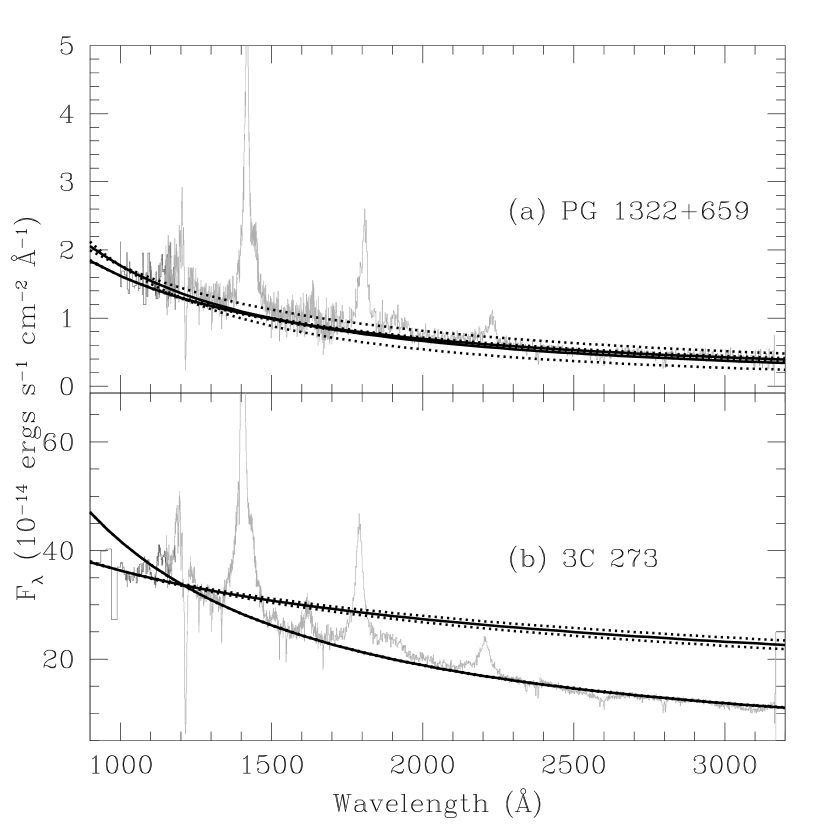
Figure 21: Comparison of HST spectra (light grey) and smoothed FUSE spectra (dark grey) of PG 1322+659 (top panel) and 3C 273 (bottom panel). The solid lines show the power law continuum fits, and the dotted lines indicate the 1$\sigma$ uncertainties on the power law index.

While the FUSE AGN do not appear to show a spectral break as an ensemble, some individual objects in the sample do show a break in the far-UV. In Figure 21, we show two examples of AGNs with both FUSE and STIS G130L+G240L spectra, one with no break between the STIS and FUSE bands, and one with a distinct break. These two examples are marked as bold crosses in Figure 20(b). In the top panel, we show the FUSE and STIS spectra of PG 1322+659, a Seyfert 1 galaxy with $z=0.168$. The UV spectrum of this AGN shows no evidence for a break, $\alpha_{EUV}=-0.58\pm 0.29$ and $\alpha_{NUV}=-0.78\pm 0.04$. Some low redshift AGN do show a spectral break, however. Kriss et al. (1999) reported a break in the spectrum of 3C 273 at $\sim$900 Å from Hopkins Ultraviolet Telescope data, and they interpreted that break as the signature of a Comptonized accretion disk spectrum (Shields 1978; Malkan & Sargent 1982). Our comparison of the FUSE and STIS spectra of this object, shown in Figure 21(b), confirm a significant break between the NUV and EUV spectral slopes: $\alpha_{EUV}=-1.60\pm 0.03$ and $\alpha_{NUV}=-0.856\pm 0.005$. Note that we simply confirm a spectral break and have not attempted a self-consistent double power law fit to the full UV continuum here. A thorough study of the EUV-to-optical spectral energy distributions of AGNs and comparisons with accretion disk models using the STIS snapshot data reported above is forthcoming (Shang et al., in preparation).

7.4 Correlation of Spectral Index with Accretion Properties

Here we investigate whether the spectral slopes of the low-redshift AGNs in the FUSE sample are correlated with observable properties of the central black hole or the mass accretion process. For 22 AGNs in the FUSE sample, we have estimates of black hole mass from Kaspi et al. (2000) and M^cLure & Dunlop (2001). This quantity is listed in column 6 of Table 1 and is plotted against the spectral indices of individual AGNs in Figure 23. We find a correlation of spectral slope with black hole mass, at 96% confidence according to the Spearman rank-order test. The trend runs in the sense that AGNs with lower black hole masses show harder spectral slopes. A linear least-squares fit gives a slope of $-0.67\pm 0.35$, shown by the line in Figure 23.

For standard, geometrically thin, optically thick accretion disks, the temperature of the disk is proportional to its luminosity and to the mass of the central black hole as: $T\sim L^{1/4}M_{BH}^{-1/2}$ (Shakura & Sunyaev 1973). Therefore, the thermal disk emission will peak further in the blue in the spectra of AGNs with lower mass black holes. Thus, the spectral index observed in the NUV will extend through the EUV, and we may expect a correlation between $\alpha$ and temperature. We show $\alpha$ versus $L^{1/4}M_{BH}^{-1/2}$ in Figure 23 and the linear least-squares fit with a slope $0.86\pm 0.91$. The slope has the expected sign, but the correlation is not statistically significant, 70%.

8 Discussion

The FUSE AGN sample is approximately one-half the size of the HST sample presented by T02, and it is distinctly different in terms of both redshift ($z_{\rm median}=0.10$ versus $z_{\rm median}=0.96$ for the HST AGNs) and luminosity (median $\log(\lambda L_{1100})=45.0$ versus median $\log(\lambda L_{1100})=45.9$). Like the Z97 and T02 HST samples, this FUSE archival sample is a heterogeneous sample of AGNs observed with FUSE for various reasons. Presumably, however, most AGNs in the sample were observed because they were known a priori to be bright in the UV, particularly in the NUV. However, we note that Figures 6 and 6 illustrate that the sample is well-populated with intrinsically low-luminosity AGNs. The EUV spectral index of the FUSE composite is significantly harder than the HST composite, $\alpha=-0.56^{+0.38}_{-0.28}$ versus $\alpha=-1.76\pm 0.12$.

In constructing our composite spectrum, we followed the methodology of Z97 and T02 by using uniform weighting for each AGN spectrum. This method prevents the overall composite spectrum from being dominated by the brightest AGN with spectra of the highest S/N, such as 3C273 ($\alpha=-1.60$). This in turn provides the best estimate of the spectrum of the average AGN (Z97) and the best comparison with the HST results of Z97 and T02.

At face value, the harder spectral slope of a composite formed from low-redshift AGNs seems to lend credence to a scenario in which the spectral break in the HST composite spectrum reported by Z97 and T02 is caused by an undercorrection for intergalactic absorption, as proposed by Binette et al. (2003). However, this scenario does not easily explain the correlation between spectral slope and AGN luminosity we report, nor does it account for the enhanced emission lines in the FUSE composite relative to the HST composite.

A more natural explanation of these results is that we are seeing a manifestation of the physical mechanism put forth to explain the Baldwin effect. This correlation is generally attributed to the tendency for low-luminosity AGNs tend to show harder ionizing continua (Zheng & Malkan 1993; Wang et al. 1998; Dietrich et al. 2002). This suggests that both the enhanced high-ionization emission line strengths and the harder continuum shape of the FUSE composite spectrum with respect to the HST composite are due to the larger fraction of relatively low-luminosity AGNs in the FUSE sample. T02 explain the excess of C iv emission in the HST composite relative to the SDSS composite (Vanden Berk et al. 2001) in the same way. The larger equivalent widths of the high-ionization emission lines O vi and Ne viii in the FUSE composite relative to the HST composite is the best evidence that the harder spectral index of the FUSE composite is not caused by any wavelength-dependent systematic error in our corrections for Galactic and intergalactic absorption. In addition, the significant correlation between individual AGN spectral slopes and luminosities for both the FUSE sample and the combined FUSE + HST samples supports the Baldwin effect interpretation.

Z97 interpreted the spectral break at 1050 Å in their HST composite, along with a depression of the flux near the Lyman limit, as the signature of a Comptonized accretion disk spectrum. Relativistic effects on the emergent spectrum from an inclined accretion disk as well as Comptonization from a hot corona can broaden an intrinsic Lyman limit break (Lee, Kriss, & Davidsen 1992). Z97 estimated a Lyman limit optical depth $\tau=0.8$ for a 10% depression in the flux. We have shown that the AGNs in this low-redshift, low-luminosity FUSE sample tend to lack such a spectral break, and we find no evidence for a depression in the spectrum blueward of the Lyman limit in the FUSE composite. From the S/N in the composite, we estimate that any spectral discontinuity is less than 10%. Using non-LTE accretion disk models with no Compton scattering, Hubeny et al. (2000) demonstrated that emission may wash out Lyman edge discontinuities in QSOs with $L\gtrsim 0.01L_{\rm Edd}$, particularly in systems with $M_{\rm BH}\lesssim 10^{9}M_{\sun}$. We calculate the Eddington ratio for the 22 FUSE AGNs for which we have estimates of black hole mass in Table 1 using that black hole mass and bolometric luminosities from Woo & Urry (2002) or Padovani & Rafanelli (1988), also listed in Table 1. The Eddington ratio is plotted versus black hole mass in Figure 24, which indicates that the FUSE AGN occupy the region of parameter space noted above. The lack of a flux discontinuity in the FUSE composite is consistent with the Hubeny et al. (2000) models in this sense. However, their models do predict a change in the spectral slope for these AGNs at wavelengths blueward of the Lyman limit, a break we do not find in the FUSE composite.

The EUV spectral slope found here for AGNs with $z\leq 0.67$ does imply a spectral break between the far UV and the soft X-rays given the soft X-ray slopes reported by Laor et al. (1997), who find $<\alpha_{x}>=-1.72\pm 0.09$ and $<\alpha_{x}>=-1.15\pm 0.14$ for radio-quiet and radio-loud low-redshift QSOs, respectively. It is consistent with the presence of a soft X-ray excess and steep soft X-ray power law to join with the 0.2-2 keV power law, as Mathews & Ferland (1987) inferred from the observed strength of He ii $\lambda$1640 emission. The hard slope of the FUSE composite may also help resolve questions raised by Korista, Ferland, & Baldwin (1997) about how a soft EUV continuum such as the one found by Z97 and T02 could account for the observed strength of this line. Neglecting any turnover in the EUV-to-soft-X-ray spectral energy distribution, the FUSE composite predicts about eight times as many photons at 4 Ryd as the $\alpha=-2$ power law these authors used to calculate He ii $\lambda$1640 equivalent widths of 0.6-0.8 Å for covering fractions of 10%. The FUSE data do not cover rest frame 1640 Å, and although He ii $\lambda$1085 emission line may be present in the emission line complex identified in the composite at 1084 Å (see § 6), this identification is uncertain. We therefore leave a more complete consideration of the implications of the FUSE EUV spectral slope on AGN emission lines for future work.

If AGNs build up black hole mass via accretion over their lifetimes, the evolutionary models of Wandel (1999a,b) predict higher mass (luminosity) AGNs will have lower temperature accretion disks and softer spectral slopes in the UV and X-rays. The absence of a spectral break in the FUSE composite can be explained by such models. Low-luminosity AGNs possess hotter accretion disks, and this shifts the UV bump and the Compton break to shorter wavelengths (Z97). The anticorrelation we find between EUV spectral slope and black hole mass estimates compiled from the literature also supports this interpretation. This is undermined somewhat by the low significance of the correlation between EUV spectral index and accretion disk temperature, estimated by $L^{1/4}M_{BH}^{-1/2}$. For AGNs accreting at the Eddington limit, $L\propto M_{BH}$ and $T\propto M_{BH}^{-1/4}$ and the significant correlation between $\alpha$ and $M_{BH}$ may directly reflect a trend of $\alpha$ and accretion disk temperature. The Eddington ratios listed in Table 1 and plotted in Figure 24 indicate that in fact most of the AGNs in the sample shine at luminosities below the Eddington limit. However, we note that the estimate we use for the accretion disk temperature is a combination of two observables. If a trend between spectral slope and disk temperature is indeed present, it could easily be swamped by the considerable uncertainties in the luminosity and black hole mass.

Finally, we discuss the dip in the composite spectrum blueward of the Ne viii emission line. Possibly, this arises from the superposition of absorption features arising from highly ionized gas along the line of sight, either intrinsic to the AGNs or in the IGM. It is unlikely to reside in intergalactic absorbers comprising the warm-hot IGM (WHIM). These absorbers have been observed in O vi in several QSO sightlines (Tripp, Savage, & Jenkins 2000; Oegerle et al. 2000; Tripp & Savage 2000; Tripp et al. 2001; Sembach et al. 2001; Savage et al. 2002). We see no corresponding dip in the flux at the position of the O vi doublet in the FUSE composite spectrum. Whether these absorbers are photoionized or collisionally ionized, it is likely that O vi/Ne viii $\gg 1$ (Tripp & Savage 2000). On the other hand, if the absorbing gas is collisionally ionized and $5.75\lesssim\log T\lesssim 6.00$, or if nonequilibrium conditions hold, the abundance of Ne viii could be appreciable, even comparable to that of O vi (Heckman et al. 2002). At such temperatures, O vii and even O viii absorption would be expected and have been observed (Nicastro et al. 2002; Mathur, Weinberg, & Chen 2003). Nonetheless, if this flux depression is attributable to Ne viii in the WHIM, the question of why we find no depression due to intervening O vi is still open. If we do attribute the dip to intervening Ne viii absorption, we may estimate the mean cosmological mass density in these absorbers using

$$\Omega_{b}(\mathrm{Ne}~{}\mathrm{\scriptstyle VIII})=\frac{\mu m_{H}H_{0}}{\rho_{c}cf(\mathrm{Ne}~{}\mathrm{\scriptstyle VIII})}\left(\frac{\mathrm{Ne}}{\mathrm{H}}\right)^{-1}$$

$$\times\frac{\sum_{i}N_{i}(\mathrm{Ne}~{}\mathrm{\scriptstyle VIII})}{\Delta X}$$ (3)

(Tripp et al. 2000), where $\mu$ is the mean atomic weight, taken to be 1.3, $f$(Ne viii) is the ionization fraction of Ne viii, and (Ne/H) is the neon abundance by number. The quantity $\sum_{i}N_{i}(\mathrm{Ne}~{}\mathrm{\scriptstyle VIII})$ is the total column density of Ne viii estimated from the apparent column density in the absorption dip in the composite. The effective optical depth of the feature implies a total column density $N(\mathrm{Ne}~{}\mathrm{\scriptstyle VIII})\sim 6\times 10^{15}{\rm cm}^{2}$, assuming optically thin absorption (Savage & Sembach 1991). The term $\Delta X$ is the total absorption distance probed by all the sample AGN assuming $q_{0}=0.5$ (Bahcall & Peebles 1969). For [Ne/H]=-1 and $f$(Ne viii)=0.2, the peak fractional abundance of Ne viii at $\log T=5.85$ (Shapiro & Moore 1976), we estimate $\Omega_{b}\sim 0.027h_{75}^{-1}$. This value is a factor of $\sim$10 larger than the more careful lower limits set from O vi absorbers (Tripp & Savage 2000; Savage et al. 2002), and it would imply that over 60% of the baryons at $z<0.7$ reside in Ne viii absorbers.

This flux depression has a symmetric appearance with a velocity extent of $\sim$10,000 km s^-1, and the centroid of the absorption lies within $\sim$17,000 km s^-1 of the Ne viii emission line. It is difficult to imagine a redshift distribution of intervening absorbers that would naturally give rise to these characteristics, which are more closely akin to broad-absorption-line (BAL) systems. It is more likely that this feature is associated with the AGNs themselves. Broad, intrinsic highly-ionized absorption from Ne viii has been observed in several high redshift QSOs (Q 0226-1024: Korista et al. 1992; SBS 1542+541: Telfer et al. 1998; and PG 0946+301: Arav et al. 1999), as have narrow associated absorption features (UM 675: Hamann et al. 1995, 1997; HS 1700+6416: Petitjean, Riediger, & Rauch 1996; J2233-606: Petitjean & Srianand 1999; and 3C 288: Hamann, Netzer & Shields 2000). We find no obvious Ne viii absorption features in any single AGN spectrum. We deliberately excluded AGNs known to be BALs from the sample, but many AGN showing narrow intrinsic UV absorption troughs associated with X-ray $``$warm absorbers”, such as Mrk 279 (Scott et al. 2004), Mrk 509 (Kriss et al. 2000a; Kraemer et al. 2003), NGC 3783 (Gabel et al. 2003), and NGC 7469 (Kriss et al. 2000b; Kriss et al. 2003) are included in the FUSE composite sample. In photoionization models of intrinsic absorbers, Ne⁷⁺ and O⁶⁺ can coexist over large regions (Hamann 1997; Wang et al. 2000). Furthermore, given solar abundances and the similar oscillator strengths of these two doublets, we might expect to find a corresponding dip in the composite from associated O vi absorption. However, the BAL in the spectrum of SBS 1542+541 shows absorption due to highly-ionized species, including Ne viii, and lacks absorption features from low-ionization species such as C iii and Si iv seen in other BALs (Telfer et al. 1998). Their results suggest that the covering fractions of various ions can be dependent upon creation ionization potential. They do find O vi absorption in this BAL system, but our selection against known BALs in the FUSE sample from features like C iv and O vi, combined with an ionization-dependent covering fraction is a plausible explanation of the flux depression blueward of Ne viii in the FUSE composite, and the lack of one blueward of O vi.

9 Summary

We summarize our results as follows:

1. We construct a composite EUV (630-1155 Å) spectrum of AGNs with $z\leq 0.67$ from archival FUSE data.

2. We find that the best-fit spectral index of the composite is $\alpha=-0.56^{+0.38}_{-0.28}$. The conservative estimate of the total error in the spectral index includes the standard deviation in $\alpha$ in 1000 bootstrap samples of the FUSE data set, uncertainties in the extinction correction applied to the FUSE spectra, and uncertainties in the column density distribution parameter of the intervening Ly$\alpha$ forest.

3. We find that O vi/Ly$\beta$ and Ne viii emission are enhanced in the FUSE composite relative to the HST composite.

4. The FUSE composite is significantly harder than the EUV portion of the HST composite spectrum of T02 who find $\alpha=-1.76\pm 0.12$ for 332 spectra of 184 AGNs with $z>0.33$.

5. We find significant correlations of EUV spectral index with redshift and luminosity in the FUSE AGN sample and in the FUSE sample combined with the sample of T02 in the sense that lower redshift/luminosity AGNs have harder spectral slopes.

6. From comparisons of the FUSE spectra with data from HST and IUE, we find no evidence for a UV spectral break at $\sim$1200 Å in the FUSE AGN sample.

7. We find a significant correlation of EUV spectral index with black hole mass for 22 AGNs for which such measurements exist in the literature. The trend of EUV spectral index with disk temperature, estimated from the AGN luminosities and black hole masses, runs in the expected direction. The correlation between these quantities is not significant, perhaps due to observational uncertainties.

8. The FUSE sample is dominated by low-redshift, low-luminosity AGNs. Therefore, items 3-7 suggest the physical underpinnings of the Baldwin effect, the tendency for lower luminosity AGNs to have hotter accretion disks and harder spectra in the UV and soft X-rays.

Table 1: AGN in FUSE Sample

Name	$z$	E(B-V)	$\log(\lambda L)$	$\alpha_{\lambda}$	Fλ	$\log{\rm M}_{\rm BH}/{\rm M}_{\sun}$	$\log(L_{\rm bol})\tablenotemark{4}$
NGC 3783	0.010	0.119	43.7	$1.30\pm 0.14$	$2.04\pm 0.03$	$7.04^{+0.42}_{-0.39}$	44.41
Mrk 352	0.015	0.061	43.1	$2.69\pm 0.42$	$2.37\pm 0.01$	$\cdots$	$\cdots$
NGC 7469	0.016	0.069	43.9	$1.76\pm 0.09$	$1.32\pm 0.01$	$6.88^{+0.43}_{-0.43}$	45.28
Mrk 79	0.022	0.071	43.6	$1.17\pm 0.41$	$0.29\pm 0.01$	$8.01^{+0.17}_{-0.24}$	44.57
Ark 564	0.025	0.060	43.3	$1.57\pm 0.18$	$0.160\pm 0.004$	$\cdots$	$\cdots$
Mrk 335	0.026	0.035	44.3	$1.68\pm 0.06$	$1.20\pm 0.01$	$6.58^{+0.16}_{-0.11}$	44.69
Mrk 290	0.030	0.015	43.5	$1.90\pm 0.23$	$0.14\pm 0.04$	$\cdots$	$\cdots$
Mrk 279	0.030	0.016	44.5	$1.91\pm 0.05$	$1.270\pm 0.007$	$\cdots$	$\cdots$
Mrk 817	0.031	0.007	44.4	$1.50\pm 0.08$	$0.87\pm 0.01$	$7.55^{+0.13}_{-0.11}$	44.99
Ark 120	0.032	0.128	44.5	$2.82\pm 0.14$	$1.25\pm 0.02$	$8.27^{+0.09}_{-0.10}$	44.91
IRAS F11431-1810	0.033	0.039	44.4	$4.03\pm 0.18$	$1.13\pm 0.02$	$\cdots$	$\cdots$
Mrk 509	0.034	0.057	44.4	$1.04\pm 0.28$	$1.34\pm 0.05$	$7.96^{+0.05}_{-0.05}$	45.03
Mrk 618	0.035	0.076	44.5	$2.51\pm 0.34$	$1.20\pm 0.06$	$\cdots$	$\cdots$
ESO 141-G55	0.036	0.111	44.8	$3.27\pm 0.14$	$2.78\pm 0.06$	$8.85^{+0.67}_{-0.43}$	45.62
Mrk 9	0.040	0.059	44.3	$0.95\pm 0.18$	$0.344\pm 0.009$	$\cdots$	$\cdots$
1H 0707-495	0.041	0.095	44.4	$3.63\pm 0.11$	$0.86\pm 0.01$	$\cdots$	$\cdots$
NGC 985	0.042	0.033	44.2	$3.10\pm 0.06$	$0.403\pm 0.003$	$\cdots$	$\cdots$
KUG 1031+398	0.042	0.015	43.3	$2.83\pm 0.27$	$0.051\pm 0.001$	$\cdots$	$\cdots$
Mrk 506	0.043	0.031	44.0	$2.42\pm 0.24$	$0.209\pm 0.007$	$\cdots$	$\cdots$
Fairall 9	0.047	0.027	43.9	$1.04\pm 0.33$	$0.172\pm 0.008$	$7.92^{+0.13}_{-0.22}$	45.23
Mrk 734	0.050	0.032	44.5	$1.37\pm 0.19$	$0.54\pm 0.01$	$\cdots$	$\cdots$
IRAS 09149-62	0.057	0.182	45.0	$4.34\pm 0.32$	$1.31\pm 0.05$	$\cdots$	$\cdots$
ESO 265-G23	0.056	0.096	44.4	$2.14\pm 0.43$	$0.38\pm 0.01$	$\cdots$	$\cdots$
3C 382	0.058	0.070	44.4	$2.48\pm 0.29$	$0.36\pm 0.01$	$\cdots$	$\cdots$
PG 1011-040	0.058	0.037	44.5	$0.67\pm 0.07$	$0.401\pm 0.003$	$\cdots$	$\cdots$
Mrk 1298	0.060	0.055	44.5	$1.14\pm 0.46$	$0.39\pm 0.02$	$\cdots$	$\cdots$
I Zw 1	0.061	0.065	44.2	$-0.51\pm 0.27$	$0.157\pm 0.006$	$\cdots$	$\cdots$
Ton S180	0.062	0.014	44.9	$1.93\pm 0.14$	$0.96\pm 0.01$	$\cdots$	$\cdots$
II Zw 136	0.063	0.044	44.6	$1.57\pm 0.31$	$0.464\pm 0.006$	$\cdots$	$\cdots$
PG 1229+204	0.063	0.027	44.4	$-1.12\pm 0.58$	$0.278\pm 0.007$	$7.93^{+0.21}_{-0.20}$	45.01
Ton 951	0.064	0.037	44.8	$0.36\pm 0.17$	$0.720\pm 0.005$	$\cdots$	$\cdots$
MR 2251-178	0.066	0.039	44.5	$0.69\pm 0.08$	$0.299\pm 0.003$	$\cdots$	$\cdots$
Ton 1187	0.070	0.011	44.4	$0.84\pm 0.59$	$0.223\pm 0.006$	$\cdots$	$\cdots$
Mrk 205	0.071	0.042	44.2	$1.76\pm 0.60$	$0.107\pm 0.003$	$\cdots$	$\cdots$
Mrk 478	0.079	0.014	44.8	$1.29\pm 0.32$	$0.443\pm 0.005$	$\cdots$	$\cdots$
VII Zw 118	0.080	0.038	44.8	$1.46\pm 0.30$	$0.427\pm 0.004$	$\cdots$	$\cdots$
PG 1211+143	0.081	0.035	45.2	$2.83\pm 0.27$	$0.868\pm 0.008$	$7.37^{+0.10}_{-0.13}$	45.81
Mrk 1383	0.086	0.032	45.2	$0.72\pm 0.08$	$1.06\pm 0.004$	$\cdots$	$\cdots$
PG 0804+761	0.100	0.035	45.7	$-0.53\pm 0.05$	$1.010\pm 0.003$	$8.21^{+0.04}_{-0.04}$	45.93
PG 1415+451	0.114	0.009	44.7	$1.88\pm 0.24$	$0.155\pm 0.003$	$\cdots$	$\cdots$
Ton S210	0.116	0.017	45.4	$-0.57\pm 0.07$	$0.790\pm 0.007$	$\cdots$	$\cdots$
RX J1230.8+0115	0.117	0.019	45.3	$-0.24\pm 0.20$	$0.63\pm 0.01$	$\cdots$	$\cdots$
Mrk 106	0.123	0.028	45.0	$-0.16\pm 0.22$	$0.280\pm 0.005$	$\cdots$	$\cdots$
Mrk 876	0.129	0.027	45.7	$-0.92\pm 0.05$	$1.070\pm 0.005$	$\cdots$	$\cdots$
PG 1626+554	0.133	0.006	45.0	$-0.04\pm 0.23$	$0.218\pm 0.004$	$\cdots$	$\cdots$
Q0045+3926	0.134	0.052	45.0	$1.10\pm 0.31$	$0.210\pm 0.005$	$\cdots$	$\cdots$
PKS 0558-504	0.137	0.044	45.5	$1.14\pm 0.06$	$0.695\pm 0.003$	$\cdots$	$\cdots$
PG 0026+129	0.142	0.071	45.3	$1.24\pm 0.16$	$0.445\pm 0.006$	$7.42^{+0.08}_{-0.09}$	45.39
PG 1114+445	0.144	0.016	44.3	$3.44\pm 0.67$	$0.033\pm 0.002$	$\cdots$	$\cdots$
PG 1352+183	0.152	0.019	44.7	$1.89\pm 0.40$	$0.080\pm 0.002$	$\cdots$	$\cdots$
MS 07007+6338	0.153	0.051	45.3	$0.68\pm 0.16$	$0.429\pm 0.004$	$\cdots$	$\cdots$
PG 1115+407	0.154	0.016	44.8	$0.89\pm 0.23$	$0.099\pm 0.002$	$\cdots$	$\cdots$
PG 0052+251	0.155	0.047	45.2	$0.90\pm 0.03$	$0.315\pm 0.005$	$8.48^{+0.13}_{-0.11}$	45.93
PG 1307+085	0.155	0.034	45.5	$0.07\pm 0.08$	$0.557\pm 0.004$	$8.52^{+0.16}_{-0.29}$	45.83
3C 273	0.158	0.021	46.4	$0.40\pm 0.03$	$3.630\pm 0.007$	$8.54^{+0.41}_{-0.41}$	47.24
PG 1402+261	0.164	0.016	45.5	$0.82\pm 0.13$	$0.431\pm 0.004$	$7.76^{+0.91}_{-0.30}\,$	45.13
PG 1048+342	0.167	0.023	45.0	$1.18\pm 0.26$	$0.138\pm 0.003$	$\cdots$	$\cdots$
PG 1322+659	0.168	0.019	45.1	$1.42\pm 0.29$	$0.177\pm 0.004$	$\cdots$	$\cdots$
PG 2349-014	0.174	0.027	45.4	$-1.08\pm 0.14$	$0.258\pm 0.003$	$9.26^{+0.91}_{-0.30}\,$	45.94
PG 1116+215	0.176	0.023	45.9	$-0.40\pm 0.03$	$0.891\pm 0.003$	$8.70^{+0.91}_{-0.30}\,$	46.02
FBQS J2155-0922	0.190	0.046	46.0	$0.02\pm 0.12$	$1.03\pm 0.01$	$\cdots$	$\cdots$
4C +34.47	0.206	0.037	45.1	$0.12\pm 0.36$	$0.099\pm 0.003$	$\cdots$	$\cdots$
PG 0947+396	0.206	0.019	45.2	$1.15\pm 0.25$	$0.155\pm 0.003$	$\cdots$	$\cdots$
HE 1050-2711	0.208	0.070	45.2	$0.55\pm 0.30$	$0.146\pm 0.004$	$\cdots$	$\cdots$
HE 1115-1735	0.217	0.037	45.6	$-0.16\pm 0.12$	$0.278\pm 0.003$	$\cdots$	$\cdots$
PG 0953+414	0.234	0.013	46.0	$0.75\pm 0.03$	$0.605\pm 0.001$	$8.21^{+0.07}_{-0.08}$	46.16
HE 1015-1618	0.247	0.078	45.4	$-1.33\pm 0.34$	$0.135\pm 0.004$	$\cdots$	$\cdots$
PG 1444+407	0.267	0.014	45.6	$0.91\pm 0.13$	$0.202\pm 0.002$	$8.54^{+0.91}_{-0.42}\,$	45.93
PKS 1302-102	0.278	0.043	45.8	$0.09\pm 0.05$	$0.280\pm 0.001$	$8.78^{+0.94}_{-0.30}\,$	45.86
HE 0450-2958	0.286	0.015	45.5	$0.79\pm 0.13$	$0.157\pm 0.002$	$\cdots$	$\cdots$
PG 1100+772	0.311	0.034	45.7	$0.22\pm 0.15$	$0.238\pm 0.005$	$\cdots$	$\cdots$
Ton 28	0.330	0.022	45.9	$1.97\pm 0.13$	$0.307\pm 0.005$	$\cdots$	$\cdots$
FBQS J083535.8+24	0.331	0.031	45.7	$2.42\pm 0.25$	$0.188\pm 0.005$	$\cdots$	$\cdots$
PG 1216+069	0.331	0.022	45.7	$1.20\pm 0.18$	$0.184\pm 0.004$	$\cdots$	$\cdots$
PG 1512+370	0.371	0.022	45.6	$2.77\pm 0.53$	$0.137\pm 0.009$	$\cdots$	$\cdots$
PG 1543+489	0.400	0.018	45.7	$0.83\pm 0.54$	$0.099\pm 0.007$	$\cdots$	$\cdots$
FBQS J152840.6+28	0.450	0.024	46.0	$0.61\pm 0.19$	$0.177\pm 0.004$	$\cdots$	$\cdots$
PG 1259+593	0.478	0.008	46.1	$0.42\pm 0.02$	$0.1810\pm 0.0004$	$\cdots$	$\cdots$
HE 0226-4110	0.495	0.016	46.4	$0.70\pm 0.04$	$0.345\pm 0.001$	$\cdots$	$\cdots$
HS 1102+3441	0.510	0.024	46.0	$2.83\pm 0.24$	$0.154\pm 0.003$	$\cdots$	$\cdots$
RX J2241.8-44	0.545	0.011	46.0	$3.47\pm 0.16$	$0.122\pm 0.002$	$\cdots$	$\cdots$
PKS 0405-12	0.573	0.058	46.9	$3.35\pm 0.08$	$1.13\pm 0.01$	$\cdots$	$\cdots$
HE 1326-0516	0.578	0.030	46.4	$-0.33\pm 0.13$	$0.141\pm 0.002$	$\cdots$	$\cdots$
HE 0238-1904	0.631	0.032	46.5	$1.61\pm 0.11$	$0.287\pm 0.003$	$\cdots$	$\cdots$
3C 57	0.669	0.022	46.4	$1.52\pm 0.14$	$0.169\pm 0.003$	$\cdots$	$\cdots$

Table 2: Fits to Full Sample and Subsample Composites

Sample	No. Spectra	No. AGNs	$\alpha$
Full sample	128	85	-0.56
$z<0.10$	65	39	-0.74
$z>0.10$	63	46	-0.74
$\log(\lambda L_{1100})<45.0$	64	40	0.19
$\log(\lambda L_{1100})>45.0$	64	45	-0.84
$E(B-V)<0.032$	65	44	-0.50
$E(B-V)>0.032$	63	41	-0.21

Table 3: Emission Lines

Line	$\lambda_{0}$ (Å)	Flux	EW (Å)
Neviii + Oiv	772	6.3 $\pm$0.3	8.4
Oiii	831	1.6 $\pm$0.3	2.4
H i Ly series + Svi	944	3.2 $\pm$0.5	5.6
Ly$\gamma$	973	1.1 $\pm$1.1	2.0
Ciii	976	1.5 $\pm$0.4	2.9
Niii	991	1.1 $\pm$0.2	2.1
Ly$\beta$	1026	6.2 $\pm$1.3	12.6
Ovi	1033	10.0$\pm$0.3	20.3
Siv	1062	1.7 $\pm$0.3	3.6
Siv	1073	0.8 $\pm$0.1	1.8
Nii + Heii + Ari	1084	0.23$\pm$0.05	0.4

Table 4: Fits to Individual AGN

				$\alpha$ vs. $\log z$		$\alpha$ vs. $\log\lambda L$
Sample	N	$\alpha_{\rm mean}$	$\alpha_{\rm med.}$	Slope	rs	Slope	rs
FUSE	85	-0.74$\pm$0.13	-0.86$\pm$0.13	-0.83$\pm$0.02	-0.31	-0.56$\pm$0.01	-0.36
FUSE + HST	164	-1.25$\pm$0.09	-1.40$\pm$0.09	-0.88$\pm$0.13	-0.45	-0.49$\pm$0.09	-0.38

Figure 1: Number of spectra used in the composite spectrum as a function of rest wavelength.

Figure 2: Signal-to-noise ratio in the composite spectrum per 1 Å bin.

Figure 3: Top panel: Composite AGN spectrum with power law continuum fit (dashed lines) and wavelength regions used in fit (solid line segments); HST composite from Telfer et al. (2002) shown for comparison. Bottom panel: Ratio of FUSE to HST composite spectra.

Figure 4: Lyman valley correction for a $z=0.1$ AGN with the parameters used by T02, and the correction used here, where $\gamma=0.15$, $\beta=2.0$ in Equ. 1. The dashed lines show how the correction changes for different $\gamma$ and $\beta$.

Figure 5: Luminosity versus redshift for FUSE and HST AGN with lines marking median redshift ($z=0.10$) and median luminosity ($\log\lambda L_{1100}=45.0$).

Figure 6: Histograms of redshifts and luminosities of FUSE and HST AGN with vertical lines marking median FUSE redshift and luminosity.

Figure 7: Composites made from spectra of AGNs with $z<0.10$ and $z>0.10$ with power law continuum fits (dashed lines) and wavelength regions used in fit (solid line segments). Overall composite with power law continuum fit shown for comparison.

Figure 8: Composites made from spectra of AGNs with $\log(\lambda L_{1100})<45.0$ and $\log(\lambda L_{1100})>45.0$ with power law continuum fits (dashed lines) and wavelength regions used in fit (solid line segments). Overall composite with power law continuum fit shown for comparison.

Figure 9: Histogram of $E(B-V)$ values for FUSE AGNs. The solid line marks the median $E(B-V)$, 0.032.

Figure 10: Distribution in redshift and 1100-Å luminosity for AGNs with $E(B-V)>0.032$ (filled triangles) and AGNs with $E(B-V)<0.032$ (crosses)

Figure 11: Composite AGN spectrum with fits to continuum (dashed line) and continuum + emission lines (solid line). See Table 3 for fit parameters.

Figure 12: Histogram of EUV spectral slopes in FUSE sample and in the combined FUSE and HST sample.

Figure 13: EUV spectral index versus $E(B-V)$ for FUSE AGNs with best linear least-squares fit.

Figure 14: EUV spectral index versus flux at 1000 Å for FUSE AGNs.

Figure 15: EUV spectral index versus redshift with best linear least-squares fit.

Figure 16: EUV spectral index versus 1100-Å luminosity with best linear least-squares fit.

Figure 17: Same as Figure 16 for both FUSE (solid squares) and HST (Radio-loud: solid circles, Radio-quiet: open squares) samples with best linear least-squares fit to FUSE sample (solid line) and best linear least-squares fit to combined FUSE + HST sample (dashed line).

Figure 18: Same as Figure 16 for both FUSE (solid squares) and HST (Radio-loud: solid circles, Radio-quiet: open squares) samples with best linear least-squares fit to FUSE sample (solid line) and best linear least-squares fit to combined FUSE + HST sample (dashed line).

Figure 19: Histograms of $\alpha_{NUV}$ and $\alpha_{EUV}$ measured from HST spectra of AGNs with $z>0.33$ by T02. See also their Figure 14.

Figure 20: (a) Histogram of spectral slopes measured with IUE for rest wavelengths 1200-2000 Å or HST for rest wavelengths 1150-3200 Å  ($\alpha_{NUV}$) and those measured with FUSE for $900<\lambda<1200$ Å ($\alpha_{FUSE}$). (b) Comparison of $\alpha_{FUSE}$ and $\alpha_{NUV}$. Filled squares denote $\alpha_{NUV}$’s measured from IUE spectra, open squares denote $\alpha_{NUV}$’s measured from HST spectra, and bold crosses mark the two AGNs shown in Figure 21. Dotted line shows $\alpha_{FUSE}=\alpha_{NUV}$.

Figure 22: EUV spectral index versus black hole mass listed in Table 1 for 21 AGNs in the FUSE sample, with best linear least-squares fit.

Figure 23: EUV spectral index versus temperature ($\sim\log(L^{1/4}M_{BH}^{-1/2})$) with best linear least-squares fit.

Figure 24: Eddington ratio versus black hole mass for 20 FUSE AGNs. See Table 1.

References

- Arav et al. (1999) Arav, N., Korista, K. T., de Kool, M., Junkkarinen, V. T., & Begelman, M. C. 1999, ApJ, 516, 27
- (2) Bahcall, J. N. & Peebles, P. J. E. 1969, ApJ, 156, L7
- Baldwin (1977) Baldwin, J. A. 1977, ApJ, 214, 679
- Binette, Rodríguez-Martínez, Haro-Corzo, & Ballinas (2003) Binette, L., Rodríguez-Martínez, M., Haro-Corzo, S., & Ballinas, I. 2003, ApJ, 590, 58
- Brotherton et al. (2001) Brotherton, M. S., Tran, H. D., Becker, R. H., Gregg, M. D., Laurent-Muehleisen, S. A., & White, R. L. 2001, ApJ, 546, 775
- (6) Cardelli, J. A., Clayton, G. C., & Mathis, J. S. 1989, ApJ, 345, 245
- (7) Clayton, G. C. & Cardelli, J. A. 1988, AJ, 96, 695
- (8) Davé, R. & Tripp, T. M. 2001, ApJ, 553, 528
- Dietrich et al. (2002) Dietrich, M., Hamann, F., Shields, J. C., Constantin, A., Vestergaard, M., Chaffee, F., Foltz, C. B., & Junkkarinen, V. T. 2002, ApJ, 581, 912
- (10) Dobrzycki, A., Bechtold, J., Scott, J., & Morita, M. 2002, ApJ, 571, 654
- (11) Espey, B. R. & Andreadis, S. J. 1999, in ASP Conf. Ser. 162, Quasars and Cosmology, ed. G. Ferland & J. Baldwin (San Francisco: ASP), 351
- Francis et al. (1991) Francis, P. J., Hewett, P. C., Foltz, C. B., Chaffee, F. H., Weymann, R. J., & Morris, S. L. 1991, ApJ, 373, 465
- (13) Gabel, J. R. et al. 2003, ApJ, 583, 178
- Green (1996) Green, P. J. 1996, ApJ, 467, 61
- Green (1998) Green, P. J. 1998, ApJ, 498, 170
- Hamann et al. (1995) Hamann, F., Barlow, T. A., Beaver, E. A., Burbidge, E. M., Cohen, R. D., Junkkarinen, V., & Lyons, R. 1995, ApJ, 443, 606
- Hamann (1997) Hamann, F. 1997, ApJS, 109, 279
- Hamann, Barlow, Junkkarinen, & Burbidge (1997) Hamann, F., Barlow, T. A., Junkkarinen, V., & Burbidge, E. M. 1997, ApJ, 478, 80
- Hamann, Netzer, & Shields (2000) Hamann, F. W., Netzer, H., & Shields, J. C. 2000, ApJ, 536, 101
- Heckman, Norman, Strickland, & Sembach (2002) Heckman, T. M., Norman, C. A., Strickland, D. K., & Sembach, K. R. 2002, ApJ, 577, 691
- Hubeny, Agol, Blaes, & Krolik (2000) Hubeny, I., Agol, E., Blaes, O., & Krolik, J. H. 2000, ApJ, 533, 710
- Kaspi et al. (2000) Kaspi, S., Smith, P. S., Netzer, H., Maoz, D., Jannuzi, B. T., & Giveon, U. 2000, ApJ, 533, 631
- Korista et al. (1992) Korista, K. T. et al. 1992, ApJ, 401, 529
- Korista, Ferland, & Baldwin (1997) Korista, K., Ferland, G., & Baldwin, J. 1997, ApJ, 487, 555
- (25) Kim, T.-S., Cristiani, S. & D’Odorico, S. 2001, A&A, 373, 757
- K (2003) Kraemer, S. B., Crenshaw, D. M., Yaqoob, T., McKernan, B., Gabel, J. R., George, I. M., Turner, T. J., & Dunn, J. P. 2003, ApJ, 582, 125
- K (2003) Kriss, G. A., Blustin, A., Branduardi-Raymont, G., Green, R. F., Hutchings, J., & Kaiser, M. E. 2003, A&A, 403, 473
- (28) Kriss, G. A. et al. 2000a, ApJ, 538, L17
- (29) Kriss, G. A., Peterson, B. M., Crenshaw, D. M., & Zheng, W. 2000b, ApJ, 535, 58
- K (1994) Kriss, G. A. 1994, in ASP Conf. Ser. 61, Astronomical Data Analysis Software and Systems III, ed. Dr. R. Crabtree, R. J. Hanisch, & J. Barnes (San Francisco: ASP), 437
- Kriss, Davidsen, Zheng, & Lee (1999) Kriss, G. A., Davidsen, A. F., Zheng, W., & Lee, G. 1999, ApJ, 527, 683
- Kuraszkiewicz et al. (2002) Kuraszkiewicz, J. K., Green, P. J., Forster, K., Aldcroft, T. L., Evans, I. N., & Koratkar, A. 2002, ApJS, 143, 257
- Laor et al. (1997) Laor, A., Fiore, F., Elvis, M., Wilkes, B. J., & McDowell, J. C. 1997, ApJ, 477, 93
- Lee, Kriss, & Davidsen (1992) Lee, G., Kriss, G. A., & Davidsen, A. F. 1992, in Testing the AGN Paradigm, ed. S. S. Holt, S. G. Neff, C. M. Urry (New York:AIP),159
- Malkan & Sargent (1982) Malkan, M. A. & Sargent, W. L. W. 1982, ApJ, 254, 22
- Mathews & Ferland (1987) Mathews, W. G. & Ferland, G. J. 1987, ApJ, 323, 456
- Mathur, Weinberg, & Chen (2003) Mathur, S., Weinberg, D. H., & Chen, X. 2003, ApJ, 582, 82
- McLure & Dunlop (2001) McLure, R. J. & Dunlop, J. S. 2001, MNRAS, 327, 199
- (39) Møller, P. & Jakobsen, P. 1990, A&A, 228, 299
- (40) Moos, H. W., et al. 2000, ApJ, 538, L1
- Netzer, Laor, & Gondhalekar (1992) Netzer, H., Laor, A., & Gondhalekar, P. M. 1992, MNRAS, 254, 15
- Nicastro et al. (2002) Nicastro, F. et al. 2002, ApJ, 573, 157
- Oegerle et al. (2000) Oegerle, W. R. et al. 2000, ApJ, 538, L23
- Padovani & Rafanelli (1988) Padovani, P. & Rafanelli, P. 1988, A&A, 205, 53
- (45) Penton, S. V., Shull, J. M., & Stocke J. T. 2000, ApJ, 544 150
- Petitjean, Riediger, & Rauch (1996) Petitjean, P., Riediger, R., & Rauch, M. 1996, A&A, 307, 417
- Petitjean & Srianand (1999) Petitjean, P. & Srianand, R. 1999, A&A, 345, 73
- (48) Sahnow, D. J., et al. 2000, ApJ, 538, L7
- Savage, Sembach, Tripp, & Richter (2002) Savage, B. D., Sembach, K. R., Tripp, T. M., & Richter, P. 2002, ApJ, 564, 631
- Schlegel, Finkbeiner, & Davis (1998) Schlegel, D. J., Finkbeiner, D. P., & Davis, M. 1998, ApJ, 500, 525
- (51) Scott, J. E., et al. 2004, ApJS, 152, 1
- Savage & Sembach (1991) Savage, B. D. & Sembach, K. R. 1991, ApJ, 379, 245
- Sembach et al. (2001) Sembach, K. R., Howk, J. C., Savage, B. D., Shull, J. M., & Oegerle, W. R. 2001, ApJ, 561, 573
- Shakura & Sunyaev (1973) Shakura, N. I. & Sunyaev, R. A. 1973, A&A, 24, 337
- Shang et al. (2003) Shang, Z., Wills, B. J., Robinson, E. L., Wills, D., Laor, A., Xie, B., & Yuan, J. 2003, ApJ, 586, 52
- Shapiro & Moore (1976) Shapiro, P. R. & Moore, R. T. 1976, ApJ, 207, 460
- Shields (1978) Shields, G. A. 1978, Nature, 272, 706
- Telfer et al. (1998) Telfer, R. C., Kriss, G. A., Zheng, W., Davidsen, A. F., & Green, R. F. 1998, ApJ, 509, 132
- (59) Telfer, R. C., Zheng, W., Kriss, G. A., & Davidsen, A. F. 2002, ApJ, 565, 773 (T02)
- Tripp & Savage (2000) Tripp, T. M. & Savage, B. D. 2000, ApJ, 542, 42
- Tripp, Savage, & Jenkins (2000) Tripp, T. M., Savage, B. D., & Jenkins, E. B. 2000, ApJ, 534, L1
- Tripp et al. (2001) Tripp, T. M., Giroux, M. L., Stocke, J. T., Tumlinson, J., & Oegerle, W. R. 2001, ApJ, 563, 724
- Vanden Berk et al. (2001) Vanden Berk, D. E. et al. 2001, AJ, 122, 549
- Wandel (1999a) Wandel, A. 1999a, ApJ, 527, 649
- Wandel (1999b) Wandel, A. 1999b, ApJ, 527, 657
- Wang, Lu, & Zhou (1998) Wang, T., Lu, Y., & Zhou, Y. 1998, ApJ, 493, 1
- Wang et al. (2000) Wang, T. G., Brinkmann, W., Yuan, W., Wang, J. X., & Zhou, Y. Y. 2000, ApJ, 545, 77
- (68) Weymann, R. J. et al. 1998, ApJ, 506, 1
- (69) Woo, J.-H. & Urry C. M. 2002, ApJ, 579 530
- Zheng, Fang, & Binette (1992) Zheng, W., Fang, L., & Binette, L. 1992, ApJ, 392, 74
- Zheng & Malkan (1993) Zheng, W. & Malkan, M. A. 1993, ApJ, 415, 517
- Zheng, Kriss, & Davidsen (1995) Zheng, W., Kriss, G. A., & Davidsen, A. F. 1995, ApJ, 440, 606
- (73) Zheng, W., Kriss, G. A., Telfer, R. C., Grimes, J. P., & Davidsen, A. F. 1997, ApJ, 475, 469 (Z97)