Dark energy cosmology with generalized linear equation of state

Abstract

Dark energy with the usually used equation of state $p=w\rho$, where $w=const<0$ is hydrodynamically unstable. To overcome this drawback we consider the cosmology of a perfect fluid with a linear equation of state of a more general form $p=\alpha(\rho-\rho_{0})$, where the constants $\alpha$ and $\rho_{0}$ are free parameters. This non-homogeneous linear equation of state provides the description of both hydrodynamically stable ($\alpha>0$) and unstable ($\alpha<0$) fluids. In particular, the considered cosmological model describes the hydrodynamically stable dark (and phantom) energy. The possible types of cosmological scenarios in this model are determined and classified in terms of attractors and unstable points by the using of phase trajectories analysis. For the dark energy case there are possible some distinctive types of cosmological scenarios: (i) the universe with the de Sitter attractor at late times, (ii) the bouncing universe, (iii) the universe with the Big Rip and with the anti-Big Rip. In the framework of a linear equation of state the universe filled with an phantom energy, $w<-1$, may have either the de Sitter attractor or the Big Rip.

1 Introduction

The astronomical observations indicate that the expansion of our Universe accelerates [1]. In the framework of the General Relativity this means that about two thirds of the total energy density of the Universe consists of dark energy: the still unknown component with a relativistic negative pressure $p<-\rho/3$. The simplest candidate for dark energy is the cosmological $\Lambda$-term or vacuum energy. During the cosmological evolution the $\Lambda$-term component has the constant (Lorentz invariant) energy density $\rho$ and pressure $p=-\rho$. However the $\Lambda$-term requires that the vacuum energy density be fine tuned to have the observed very low value. For this reason the different forms of dynamically changing dark energy with an effective equation of state $w\equiv p/\rho<-1/3$ were proposed instead of the constant vacuum energy density. As a particular example of dark energy, the scalar field with some a slow rolling potential (quintessence) [2] is often considered. The possible generalization of quintessence is a $k$-essence [3], the scalar field with a non-canonical Lagrangian.

Present observation data constrain the range of equation-of-state of a dark energy as $-1.38<w<-0.82$ [4]. Recently the Chandra observations [5] gave the similar restrictions on the value of $w$. These data do not exclude the possibility of our universe to be filled with a phantom energy [6]: the energy with a super-negative equation of state $w<-1$ (note, however, that the dark energy with the equation of state $w$ evolving from the quintessence-like $w>-1$ in past, to phantom-like $w<-1$ at present, provides the best fit for supernova data [7]). The different aspects of phantom cosmology were considered in [8]. The phantom energy is usually associated with the phantom or ghost fields — the scalar fields with wrong-sign kinetic term. It is known that such fields are unstable due to quantum instability of vacuum, unless the kinetic term stabilized by the ultra-violet cutoff [9]. The intriguing possibility of constructing of effective $w<-1$ from the scalar field with correct-sign kinetic term was proposed in [10]. In [11] the authors constructed the theory with the effective $w<-1$ in the braneworld models.

The presence of phantom energy in the universe leads to the interesting physical phenomena: the possibility of the Big Rip scenario [6], the black hole mass decreasing by phantom energy accretion [13] and a new type of wormhole evolution [14]. The alternatives to a scalar field model are the perfect fluid models such as a Chaplygin gas [15]. Hao and Li [16] demonstrated that $w=-1$ state is an attractor for the Chaplygin gas and equation of state of this gas could approach to this attractor from the either $w<-1$ or $w>-1$ sides.

In this paper we analyze the perfect fluid model with a general linear equation of state $p=\alpha(\rho-\rho_{0})$ where $\alpha$ and $\rho_{0}$ are constants. This is a generalization of a homogeneous linear equation of state ($\rho_{0}=0$) and is suitable for the modelling either the linear gas with $p>0$ or the dark energy with $p<0$. The advantage of the use of the general linear equation of state is the possibility to describe the dark energy with a positive squared sound speed (for the usually considered equation of state $p=w\rho$ the dark energy is hydrodynamically unstable, because $\partial p/\partial\rho=w<0$). The considered linear model is reduced to the perfect fluid model with $w=const$ at the particular case of $\rho_{0}=0$.

In the framework of this model it is possible to find analytical cosmological solutions for the arbitrary values of parameters $\alpha$ and $\rho_{0}$. We show below that this linear model (unlike the Chaplygin gas model) describes distinctively different types of cosmological scenarios: the Big Bang, Big Crunch, Big Rip, anti-Big Rip, solutions with de the Sitter attractor, bouncing solutions, and their various combinations.

The paper is organized as follows. The principal part of the paper is Sec. 2 in which the basic properties and particular analytical solutions for a perfect fluid cosmology with a linear equation of state are derived. We show that dark energy with the equation of state $p=\alpha(\rho-\rho_{0})$ may be effectively reduced to the $\Lambda$-term and to the simplified linear equation of state $p_{\rm eff}=w_{\rm eff}\rho_{\rm eff}$. In this case, either the effective density $\rho_{\rm eff}$ or the density of an effective $\Lambda$-term may in general have the negative values. In dependence of signs of parameters $\alpha$ and $\rho_{0}$ the four different cosmological scenarios are considered. To study the cosmological dynamics of the universe for different scenarios the phase plane analysis is used. In Sec. 3 we discuss the restrictions which can be set on this cosmological model from the astronomical observations. The discussion of the results and their further possible generalization is presented in Sec. 6.

2 Linear equation of state

We consider the flat Friedman-Robertson-Walker universe filled with a perfect fluid. For the sake of simplicity we will call below this fluid as dark energy. Using the unit conventions $8\pi G/3=c=1$ the corresponding Einstein equations for this cosmology can be written as follows:

$$H^{2}=\rho_{\rm DE},$$ (1)

$$\dot{\rho}_{\rm DE}=-3H(\rho_{\rm DE}+p_{\rm DE}),$$ (2)

where $H=\dot{a}/a$ is the Hubble parameter and $\rho_{\rm DE}$ and $p_{\rm DE}$ are the energy density and pressure of a dark energy correspondingly. In this paper we consider a perfect fluid with the linear equation of state of the following general form:

$$p_{\rm DE}=\alpha(\rho_{\rm DE}-\rho_{0}),$$ (3)

where $\alpha$ and $\rho_{0}$ are constants. Certain features of cosmology with $\rho_{0}\neq 0$ and $0<\alpha<1$ was considered in [12]. The equation of state (3) was used in [13] to describe the dark energy accretion onto the black hole. Note the difference of this equation of state (3) from the commonly used one $p=w\rho$ with $w=const$. Our simple generalization allows to include dark (and also phantom) energy with a positive squared sound speed of linear perturbations $c_{s}^{2}\equiv\partial p/\partial\rho=\alpha\geq 0$.

One can use the observational restrictions [4] on the allowable range of equation of state, $-1.38<w<-0.82$, to put the restrictions on the parameters of a linear model (3). Substituting (3) into the equation of state $w=p_{\rm DE}/\rho_{\rm DE}$ we obtain the range of allowable parameters parameters $\alpha$ and $\rho_{0}$, shown in the Fig. (1).

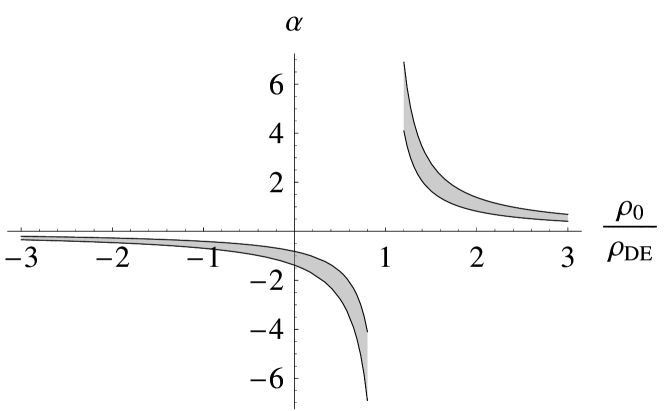
Figure 1: Observational restrictions [4] on the allowable of the equation of state, $-1.38<w<-0.82$ recalculated and presented for parameters $\alpha$ and $\rho_{0}$ of the linear model of dark energy. Here $\alpha$ and $\rho_{0}$ are the parameters in (3) and $\rho_{\rm DE}$ is the present density of dark energy.

The equation of state (3) can be reduced to the “effective” cosmological constant and the dynamically evolving dark energy by redefining the fluid density and pressure in the following way:

$$\rho_{\rm DE}=\rho_{\Lambda}+\rho_{\alpha},\quad p_{\rm DE}=p_{\Lambda}+p_{\alpha},$$ (4)

where

$$p_{\Lambda}=-\rho_{\Lambda},\quad p_{\alpha}=\alpha\rho_{\alpha},$$ (5)

and

$$\rho_{\Lambda}=\frac{\alpha\rho_{0}}{1+\alpha},\quad\rho_{\alpha}=\rho_{\rm DE}-\frac{\alpha\rho_{0}}{1+\alpha}.$$ (6)

In Eqs. (4,5,6) we denote $\rho_{\Lambda}$ and $p_{\Lambda}$ as the density and the pressure of the ”effective” cosmological constant. Correspondingly, $\rho_{\alpha}$ and $p_{\alpha}$ are the density and pressure of the dynamically evolving part of dark energy. The values $\rho_{\Lambda}$ and $p_{\Lambda}$ obviously obey the relation $\dot{\rho}_{\Lambda}=-3H(\rho_{\Lambda}+p_{\Lambda})$ and therefore $\rho_{\alpha}$ and $p_{\alpha}$ obey the equation:

$$\dot{\rho}_{\alpha}=-3H(\rho_{\alpha}+p_{\alpha}).$$ (7)

The cosmology with $\Lambda$-term and a linear equation of state (for $p/\rho>-1$) was considered previously in [17]. Note, however, that in our consideration either $\rho_{\Lambda}$ or $\rho_{\alpha}$ may be negative (nevertheless the sum $\rho_{\Lambda}+\rho_{\alpha}$ must be positive) and also equation of state for dynamically changing part of dark energy may be super-negative. This leads to the new distinctive types of cosmological scenarios considered below. The signs of $\rho_{\alpha}$ and $\rho_{\Lambda}$ are conserved during the universe evolution as can be seen from (7) and (2). Below we obtain the full analytical solutions of evolution of the universe. In both cases $\rho+p>0$ and $\rho+p<0$ we find from (7) and (2):

$$\rho_{\alpha}=\frac{A}{a^{3(1+\alpha)}},$$ (8)

where constant $A$ may be either positive or negative. Two different asymptotic regimes are possible: for $|\rho_{\alpha}|\ll|\rho_{\Lambda}|$ the universe behaves like the de Sitter universe with

$$\rho\approx\rho_{\Lambda},\quad p\approx-\rho_{\Lambda},$$ (9)

and for $|\rho_{\alpha}|\gg|\rho_{\Lambda}|$ the universe is filled with dynamical part of dark energy:

$$\rho\approx\rho_{\alpha}.$$ (10)

Using (1) and (8) we obtain the relation between the differentials $da$ and $dt$:

$$\frac{da}{a\sqrt{\rho_{\Lambda}+Aa^{-3(1+\alpha)}}}=\pm dt.$$ (11)

In dependence on signs of $\rho_{\Lambda}$ and $A$ there can be three different results for integration of relation (11). For $\rho_{\Lambda}>0$ and $A>0$ we find:

$$a(t)=\left\{\sqrt{\beta}\;\sinh\left[\pm\frac{\kappa}{2}\sqrt{\rho_{\Lambda}}\;t\right]\right\}^{2/\kappa}.$$ (12)

Here we denote $\kappa=3(1+\alpha)$ and $\beta=A/\rho_{\Lambda}$. The choice of the upper or lower sign in (12) depends on the sign ”$+$” or ”$-$” in (11). The expression (12) was first obtained in [17]. The asymptotic behavior of (12) for $t\to 0$ is given by

$$a=\left(\pm\frac{\kappa}{2}\sqrt{A}\;t\right)^{2/\kappa},$$ (13)

The Eq. (12) for $t\to\pm\infty$ can be rewritten as follows:

$$a=\left(\frac{|\beta|}{4}\right)^{1/\kappa}\exp\left(\pm\sqrt{\rho_{\Lambda}}\;t\right),$$ (14)

The expression (14) is valid only if $\kappa>0$. For $\kappa<0$ the signs in exponent in this expression should be changed to opposite ones.

In the case $\rho_{\Lambda}>0$ and $A<0$ the integration of (11) gives:

$$a(t)=\left\{\sqrt{-\beta}\;\cosh\left[\frac{\kappa}{2}\sqrt{\rho_{\Lambda}}\;t\right]\right\}^{2/\kappa}.$$ (15)

In slightly different form the solution (15) was obtained in [18] for the restricted case $-1<\alpha<0$. The asymptotic behavior of a scale factor for $t\to 0$ is given by:

$$a(t)=(-\beta)^{1/\kappa}\left(1+\frac{\kappa}{4}\;\rho_{\Lambda}\;t^{2}\right).$$ (16)

For $t\to\pm\infty$ the scale factor evolution is described by (14). Finally, for $\rho_{\Lambda}<0$ and $A>0$ one can find the evolution of the scale factor of the universe:

$$a(t)=\left\{\sqrt{-\beta}\;\sin\left[\frac{\kappa}{2}\sqrt{-\rho_{\Lambda}}\;t\right]\right\}^{2/\kappa}.$$ (17)

In the limitation $-1<\alpha<1$ the similar solution was found in [19] for the cosmology with negative anti-de Sitter $\Lambda$-term plus a scalar quintessential field with special form of a potential. For $t\to 0$ the asymptotic behavior of scale factor is given by (13). The behavior of a scale factor near $t\simeq\pi/(\kappa\rho_{\Lambda})$ can be described as follows:

$$a(t)=\left\{\sqrt{-\beta}\;\left[1-\frac{1}{2}\left(\frac{\kappa}{2}\sqrt{-\rho_{\Lambda}}\;t-\frac{\pi}{2}\right)^{2}\right]\right\}^{2/\kappa}.$$ (18)

Correspondingly, the asymptotic behavior of scale factor at $t\to\pm 2\pi/(\kappa\rho_{\Lambda})$ is given by

$$a=\left(\pi\sqrt{-\beta}-\frac{\kappa}{2}\sqrt{A}\;t\right)^{2/\kappa}.$$ (19)

To find the attractors and unstable points of the solution of the Friedman equations we use the method of the phase trajectories. Denoting $y=\rho_{\alpha}+p_{\alpha}$ we obtain the following system of equations

$$\dot{H}=-3y/2,\quad\dot{y}=-3(\alpha+1)Hy.$$ (20)

All phase trajectories of the system lie on the curve $H^{2}=\rho_{\rm DE}$ which can be rewritten as $y=(\alpha+1)H^{2}-\alpha\rho_{0}$. The particular form of this curve and direction of the phase trajectory depends on the signs of $1+\alpha$ and $\alpha\rho_{0}$. The four cases are possible:

(i) $1+\alpha>0$ and $\alpha\rho_{0}>0$.

There are two singular points at $y=0$ axis. At the point ($H=\rho_{\Lambda}^{1/2}$, $y=0$) the linearized system of evolution equations is

$$\dot{H}=-3y/2,\quad\dot{y}=-3(1+\alpha)\rho_{\Lambda}^{1/2}y,$$ (21)

The first eigenvalue and the first eigenvector of the system equal to zero. The second eigenvalue equals to $\lambda_{2}=3(1+\alpha)\rho_{\Lambda}^{1/2}<0$ and the second eigenvector is $\{3/2,3(1+\alpha)\rho_{\Lambda}^{1/2}\}$. We can see that the considered point is the attractor. The same linearization method is used for the universe evolution analysis near other singular points. The second singular point ($H=-\rho_{\Lambda}^{1/2}$, $y=0$) corresponds to the unstable equilibrium state. The another interesting singular point is ($H=0$, $y=-\alpha\rho_{0}$), in which the universe reaches the zero density $\rho_{\rm DE}=0$ and its contraction is changed to the expansion. The phase trajectories near the singular points are plotted in the left panel of Fig. 2 with the directions of evolution marked by arrows. In the auxiliary right panel of Fig. 2 the evolution of pressure $p$ as a function of the dark energy density $\rho$ is shown.

The right branch of parabola in the left panel of Fig. 2 ($y>0$, $H>0$) corresponds to the solution (12) with an upper sign at $t>0$. In this case the universe is filled with non-phantom energy. The universe starts from the Big Bang, corresponding to the initial values of density $\rho_{{\rm DE},i}=+\infty$ and scale factor $a_{i}=0$. The asymptotic behavior of a scale factor at $a\to 0$ is described by (13) with an upper sign. The relation (13) with an upper sign describes also the evolution of a scale factor for $\rho_{\Lambda}=0$ for all $t$. At the late times the universe approaches to the de Sitter regime (9). The sign of $\rho+p$ is conserved during the evolution of the universe. The asymptotic behavior of $a$ for $t\to\infty$ is given by (14) with an upper sign. The left branch of parabola in left panel of Fig. 2 ($y>0$, $H<0$) corresponds to the reverse process with respect to the examined above and is described by (12) with a lower sign. Note that $t$ is taken to be negative in this case. The asymptotic behavior for $t\to 0$ and ($t\to\infty$) is given by (13) and (14) correspondingly with lower sighs in both cases. A middle part of the parabola in left panel of Fig. 2 ($y<0$) corresponds to the solution (15). This particular case was considered in [18] as a simplest example of phantom cosmology without a Big Rip. The universe in this case is filled with a phantom energy. Because of the specifics of a linear equation of state, the considered universe with a phantom energy is not born in the Big Bang. Instead of this, the universe starts in this case from the initial scale factor $a_{i}=+\infty$. For $t\to-\infty$ it behaves like the de Sitter universe (however reversed in time) according to (14) with an upper sign and bounces at the minimal value of a scale factor $a_{min}=(-\beta)^{1/\kappa}$. In this moment the state of dark energy is very special: the pressure is finite but the total energy density is zero, $\rho_{\alpha}+\rho_{\Lambda}=0$. Near the bounce this universe can be described by (16). After the bouncing the universe expands and at the late times it approaches to the de Sitter state (14) with an upper sign.

Figure 2: Phase trajectory of the universe and diagram of evolution in coordinates ($p$, $\rho$) are shown in the case of dark energy parameters $1+\alpha>0$ and $\alpha\rho_{0}>0$. In the left panel the phase space diagram of evolution in coordinates $H$ and $y\equiv\rho_{\alpha}+p_{\alpha}$ is presented. The direction of evolution is shown by arrows. There are two unstable singular points, ($H=-\rho_{\Lambda}^{1/2}$, $y=0$) and ($H=0$, $y=-\alpha\rho_{0}$), and one attractor ($H=\rho_{\Lambda}^{1/2}$, $y=0$). In the right panel the evolution of is shown in coordinates $\rho$ and $p$. The evolution from $\rho=\infty$ to $\rho=\rho_{\Lambda}$ corresponds to the right branch of parabola ($y>0$, $H>0$) of the phase space diagram. The reverse process (from $\rho=\rho_{\Lambda}$ to $\rho=\infty$) corresponds to the left branch of parabola ($y>0$, $H<0$) of phase space diagram. The evolution from $\rho=\rho_{\Lambda}$ to bounce $\rho=0$ and back to $\rho=\rho_{\Lambda}$ corresponds to the middle branch of parabola ($y<0$) of phase space diagram.

(ii) $1+\alpha>0$ and $\alpha\rho_{0}<0$.

Figure 3: Phase trajectory of the universe and diagram of evolution in coordinates ($p$, $\rho$) are shown in the case of dark energy parameters $1+\alpha>0$ and $\alpha\rho_{0}<0$. In the left panel the phase space diagram of evolution in coordinates $H$ and $y\equiv\rho_{\alpha}+p_{\alpha}$ is presented. The direction of evolution is shown by arrows. There is only one singular point, ($H=0$, $y=-\alpha\rho_{0}$), which is unstable. In the right panel the evolution is shown in coordinates $\rho$ and $p$. The universe evolves from $\rho=\infty$ to $\rho=0$, which corresponds to the right branch of parabola ($H>0$) of the phase space diagram. At the point $\rho=0$ (corresponding to the point ($H=0$, $y=-\alpha\rho_{0}$) of the phase space diagram) there is a bounce. Then the universe evolves back to $\rho=\infty$ which corresponds to the left branch of parabola ($H<0$) of the phase space diagram.

The density of the $\Lambda$-term is negative, $\rho_{\Lambda}<0$. The linearized system of the evolution equations at the point ($H=0$, $y=-\alpha\rho_{0}$) is

$$\dot{H}=3\alpha\rho_{0}/2-3(y+\alpha\rho_{0})/2,\quad\dot{y}=3(1+\alpha)\alpha\rho_{0}H.$$ (22)

Universe expands starting from the Big Bang, reaches the zero density at the point ($H=0$, $y=-\alpha\rho_{0}$) and then its expansion changes to the contraction. The phase trajectory and diagram of evolution $p-\rho$ are shown in the Fig. 3 (the similar cosmological behavior was obtained in [19] for the universe with negative $\Lambda$-term and quintessence with special potential). The universe is filled with non-phantom energy and starts from the Big Bang. The evolution of a scale factor is described by (17) and at early times by the asymptotic (13) with an upper sign. This asymptotic is also valid for $\rho_{\Lambda}=0$ at all $t$. During the finite time $\Delta t=\pi/(\kappa\rho_{\Lambda})$ a scale factor $a$ reaches the maximum value $a_{max}=(-\beta)^{1/\kappa}$ at which the universe bounces. Near the bounce the behavior of a scale factor can be described by (18). After the bounce the universe contracts and in a finite time $\Delta t$ it collapses to the Big Crunch. The scale factor of the universe near the collapse is given by (19).

(iii) $1+\alpha<0$ and $\alpha\rho_{0}<0$.

Figure 4: Phase trajectory of the universe and diagram of evolution in coordinates ($p$, $\rho$) are shown in the case of dark energy parameters $1+\alpha<0$ and $\alpha\rho_{0}<0$. In the left panel the phase space diagram of evolution in coordinates $H$ and $y\equiv\rho_{\alpha}+p_{\alpha}$ is presented. The direction of evolution is shown by arrows. There are two unstable singular points, ($H=\rho_{\Lambda}^{1/2}$, $y=0$) and ($H=0$, $y=-\alpha\rho_{0}$), and one attractor ($H=-\rho_{\Lambda}^{1/2}$, $y=0$). In the right panel evolution of the universe is shown in coordinates $\rho$ and $p$. The evolution from $\rho=\rho_{\Lambda}$ to $\rho=\rho_{\infty}$ corresponds to the right branch of parabola ($y<0$, $H>0$) of the phase space diagram. The reverse process from $\rho=\infty$ to $\rho=\rho_{\Lambda}$ corresponds to the left branch of parabola ($y<0$, $H<0$) of phase space diagram. The evolution from the $\rho=\rho_{\Lambda}$ to bounce at $\rho=0$ and back to $\rho=\rho_{\Lambda}$ corresponds to the middle branch of parabola ($y>0$) of phase space diagram.

At the zero density in the point ($H=0$, $y=-\alpha\rho_{0}$) the universe expansion is changed to the contraction. The singular point ($H=-\rho_{\Lambda}^{1/2}$, $y=0$) is an attractor and respectively ($H=\rho_{\Lambda}^{1/2}$, $y=0$) is an unstable equilibrium point. The phase trajectory and diagram of evolution $p-\rho$ are shown in the Fig. 4.

First we consider the right branch of the parabola ($y<0$, $H>0$). In this case the universe is filled with phantom energy, $\rho+p<0$. The evolution of a scale factor is given by (12) with an upper sign. Note that $t$ is taken to be negative in this case. Starting from the scale factor $a_{i}=0$ the universe expands during an infinite time to the final Big Rip. At $t\to-\infty$ a scale factor of the universe is given by (14) with an upper sign. Near the Big Rip a scale factor $a$ is described by (13) with an upper sign (note that $\kappa$ and $t$ are both negative). The left branch of the parabola ($y<0$, $H<0$) corresponds to the reverse process with respect to the examined above and is described by (12) with a lower sign. Time $t$ is positive during the whole evolution. In this case the universe is filled with phantom energy and it starts from the ”anti-Big Rip” solution (with the infinite value of the initial scale factor), contracts during an infinite time to the final $a_{f}=0$. The asymptotic behavior for $t\to 0$ and $t\to+\infty$ is given by (13) with the lower sign and (14) with the lower sign correspondingly. The middle part of the parabola ($y>0$) corresponds to the solution (15). The universe is filled with a non-phantom energy and starts from $a_{i}=0$. At $t\to-\infty$ the scale factor of the universe is given by (14) with the upper sign. After the bouncing at the maximum value of a scale factor $a_{max}=(-\beta)^{1/\kappa}$ the universe begins to contract. Near the bouncing point the scale factor is given by (16). At $t\to+\infty$ the universe behaves like (14) with the lower sign.

(iv) $1+\alpha<0$ and $\alpha\rho_{0}>0$.

In this case the density of the $\Lambda$-term is negative: $\rho_{\Lambda}<0$. The universe reaches the zero density at the point ($H=0$, $y=-\alpha\rho_{0}$), where the contraction is changed to the expansion. The phase trajectory and diagram of evolution $p-\rho$ is shown in the Fig. 5. The universe is filled with a phantom energy and the solution for a scale factor is given by (17). The universe is born in the ”anti-Big Rip” state and the scale factor is given by (13) with the lower sign near $t\approx 0$. Then the universe contracts to the minimum state $a_{min}=(-\beta)^{1/\kappa}$ in a finite time $\Delta t=\pi/(\kappa\rho_{\Lambda})$, and after bouncing it begins to expand. In time $\Delta t$ the universe comes to the Big Rip where the scale factor of the universe is given by (19).

Different cosmological scenarios discussed above in this Section are summarized in Table 1.

Figure 5: Phase trajectory of the universe and diagram of evolution in coordinates ($p$, $\rho$) are shown in the case of dark energy parameters $1+\alpha<0$ and $\alpha\rho_{0}>0$. In the left panel the phase space diagram of evolution in coordinates $H$ and $y\equiv\rho_{\alpha}+p_{\alpha}$ is presented. The direction of evolution is shown by arrows. There is only one singular point, ($H=0$, $y=-\alpha\rho_{0}$), which is unstable. In the right panel the evolution of the universe is shown in coordinates $\rho$ and $p$. The universe evolves from ”anti-Big Rip” state ($\rho=\infty$) to the bouncing point ($\rho=0$), which corresponds to the left branch of parabola ($H<0$) of the phase space diagram. Then the universe evolves to the Big Rip ($\rho=\infty$) which corresponds to the right branch of parabola ($H>0$) of the phase space diagram.

3 Universe with dark energy and matter

If we add the usual matter (dark matter, baryons and radiation) to the considered universe then the differential equation for a scale factor evolution would have the following form:

$$\left(\frac{\dot{a}}{a}\right)^{2}=H_{0}^{2}[\Omega_{r,0}(1+z)^{4}+\Omega_{m,0}(1+z)^{3}+\Omega_{\Lambda,0}+\Omega_{\alpha,0}(1+z)^{3(\alpha+1)}],$$ (23)

where $H_{0}$ is the current value of the Hubble constant, $z=a_{0}/a-1$ is a redshift, $\Omega_{r,0}$ and $\Omega_{m,0}\simeq 0.3$ are the cosmological density parameters of radiation and non-relativistic matter correspondingly. The value of the cosmological density parameter of ”$\Lambda$-term” is: $\Omega_{\Lambda,0}=[\alpha/(\alpha+1)]\rho_{0}/\rho_{c,0}$, where $\rho_{c,0}$ is the current critical density. The contribution of the dynamically changing part of dark energy is the following: $\Omega_{\alpha,0}=\Omega_{q,0}-\Omega_{\Lambda,0}$, where $\Omega_{q,0}\simeq 0.7$ is the quintessence density parameter. We suppose that the universe is flat with $\Omega_{r,0}+\Omega_{m,0}+\Omega_{q,0}=1$. In the case of pure $\Lambda$-term ($\alpha=-1$, $\rho_{0}=0$), one should omit the last term in the brackets in (23) and take $\Omega_{\Lambda,0}=\Omega_{q,0}$.

Table 1: Possible cosmological scenarios in the case of a generalized linear equation of state $p=\alpha(\rho-\rho_{0})$ depending on parameters $\alpha$ and $\rho_{0}$.

Values of $H=\dot{a}/a$	$1+\alpha>0$, $\alpha\rho_{0}>0$	$1+\alpha>0$, $\alpha\rho_{0}<0$	$1+\alpha<0$, $\alpha\rho_{0}<0$	$1+\alpha<0$, $\alpha\rho_{0}>0$
$H<-\sqrt{\rho_{\Lambda}}$	Contraction		Contraction
$H=-\sqrt{\rho_{\Lambda}}$	Non-steady equilibrium point	Expansion, bounce and contraction	Attractor	Contraction from the anti-Big Rip,
$-\!\sqrt{\rho_{\Lambda}}\!<\!H\!<\!\sqrt{\rho_{\Lambda}}$	Contraction, bounce and expansion		Expansion, bounce and contraction	bounce and expansion to the Big Rip
$H=\sqrt{\rho_{\Lambda}}$	Attractor		Non-steady equilibrium point
$H>\sqrt{\rho_{\Lambda}}$	Expansion		Expansion

The observational restrictions on the $w$ ($-1.38<w<-0.82$), derived from the SN data, limit only the behavior of the universe at small redshifts $z\simeq 0-1$. In the case of $\rho_{0}/\rho_{\rm DE}<1$ (see Fig. 1) the dark energy does not change drastically the evolution of the universe at high redshift in comparison with a pure $\Lambda$-term case. The only restriction is the age of the universe which is limited (e.g. by the oldest globular clusters) to $t_{0}>12\cdot 10^{9}$ yr. We find the age of the universe in our model by integration of (23) from $z=0$ to $z=\infty$ for different values of $\alpha$ and $\rho_{0}$ and for nowadays values of $H_{0}=65$ km s^-1 Mpc^-1, $\Omega_{m}=0.3$ and $\Omega_{r}=4.54\cdot 10^{-5}/h^{2}$, where $h$ is the $H_{0}$ in the units $100$ km s^-1 Mpc^-1. The connection of commonly used parameter $w$ with our parameters $\alpha$ and $\rho_{0}$ is given by relation $w=\alpha(1-\rho_{0}/\rho_{\rm DE})$. For example, if $w=-0.82$ then the age restriction is important only at $\rho_{0}/\rho_{\rm DE}\leq-100$. In the case of $w<-1$ the universe is older then in a pure $\Lambda$-term case ($w=-1$) and the age restriction is unimportant.

In contrast, at $\rho_{0}/\rho_{\rm DE}>1$ only a small range of parameters may correspond to the real universe. In addition to restriction on $w$ and the universe age restriction one must require the universe to start from the Big Bang and not from the bounce at a finite scale factor. The bounce $\dot{a}=0$ appears in the case of $\alpha>1/3$ and $\Omega_{\alpha,0}<0$. Therefore, to avoid the bounce we must additionally require that $\alpha\leq 1/3$. One more condition $\Omega_{\alpha,0}+\Omega_{r,0}>0$ should be satisfied in the boundary case of $\alpha=1/3$. Strictly speaking, the bounce at redshift $1+z_{b}=(\Omega_{r,0}/|\Omega_{\alpha,0}|)^{1/(3\alpha-1)}$ could not occur later then the end of inflation or reheating moment at the temperature $T_{\rm RH}\sim 10^{13}$ GeV corresponding to $z_{\rm RH}\sim 10^{26}$. Therefore it is necessary to satisfy the condition $z_{b}\gg z_{\rm RH}$. The last condition puts the restriction to the allowable values of $\alpha$ and $\Omega_{\alpha,0}$. This restriction can be considered in the particular inflation model with taking into account the additional dynamical components (say inflaton). This consideration is out of scope of this paper.

4 Discussion and Conclusion

Figure 6: The evolution of dark energy with an arbitrary equation of state $p(\rho)$ is shown. The curves $p=p(\rho)$ are the generalization of a linear equation of state, shown in Figures (2), (3), (4) and (5). Near each point of a sufficiently smooth curve $p=p(\rho)$ one can represent the curve by its linear approximation thus reducing to the results of Section (2).

In this paper we examined the dynamical evolution of the universe filled with a dark energy obeying the linear equation of state (3). It turns out that this simple linear model for the different choices of parameters $\alpha$ and $\rho_{0}$ has a rich variety of cosmological dynamics. In dependence on signs of $1+\alpha$ and $\alpha\rho_{0}$ and the initial conditions for $\rho$ and $p$ there can be a set of distinctive types of the cosmological scenarios: Big Bang, Big Crunch, Big Rip, anti-Big Rip, solutions with the de Sitter attractor, bouncing solutions, and their various combinations. In the framework of the linear model (3) the analytical solutions of the dynamics of the universe were obtained. Using the phase plane analysis we gave the full classification of the solutions in dependence on the parameters $\alpha$ and $\rho_{0}$.

We distinguish four main types of the evolution of the universe filled with dark energy with a linear equation of state (3):

(i) For parameters $1+\alpha>0$ and $\alpha\rho_{0}>0$ the universe may contain either non-phantom or phantom energy. For the non-phantom energy there are two types of evolution: a) starting from the Big Bang the universe approaches to the de Sitter phase during an infinite time; b) reversed process with respect to the described above when the universe starts from a reversed in time the de Sitter phase and evolves to the Big Crunch. In the phantom case the universe starts from the reversed in time the de Sitter phase then it riches the bouncing point ($\rho=0$, $p\neq 0$) and after bounce the universe approaches to the de Sitter phase.

(ii) For parameters $1+\alpha>0$ and $\alpha\rho_{0}<0$ the universe may contain only non-phantom energy. In this case the only one type of evolution is possible: the universe expands starting from the Big Bang, reaches the bounce point ($\rho=0$, $p\neq 0$) in finite time and then its expansion changes to the contraction, resulting in the Big Crunch.

(iii) For parameters $1+\alpha<0$ and $\alpha\rho_{0}<0$ the universe may contain either non-phantom or phantom energy. In the case of phantom universe there are two possible scenarios: a) starting from $a_{i}=0$ the universe expands in infinite time to the final Big Rip; b) the reversed in time process with respect to the described above when the universe starts from the anti-Big Rip and evolves to final state with $a_{f}=0$. In the non-phantom case the universe starts from the reversed in time the de Sitter phase. Then it reaches the bouncing point ($\rho=0$, $p\neq 0$) and after the bounce the universe approaches the de Sitter phase.

(iv) For parameters $1+\alpha<0$ and $\alpha\rho_{0}>0$ the universe may contain only phantom energy. The universe is born in the anti-Big Rip state and contracts reaching the bouncing point in a finite time. After the bouncing the universe begins to expand. In a finite time the universe comes to the Big Rip.

The Table 1 summarizes the above results for the evolution of the universe filled with dark energy with a generalized equation of state (3).

It should be stressed that the linearity of a considered dark energy equation of state is not crucial for the general properties of cosmological evolution. Instead of (3), one may consider any the rather smooth curves $p=p(\rho)$ as shown in Fig. (6). It is clear that the general behavior of the evolution and properties of attractors and bounce points do not change in this case because any sufficiently smooth function $p=p(\rho)$ can be linearized in the local vicinity of any point. Thus we can reduce the general problem for $p=p(\rho)$ to the analysis of a linear cosmology considered in this paper. From the above it follows in particular that the universe filled with a dark energy with an equation of state $p_{\rm DE}=p_{\rm DE}(\rho_{\rm DE})$ always approaches the de Sitter attractor if additionally the physically reasonable conditions $0<dp_{\rm DE}/d\rho_{\rm DE}<1$ is satisfied. The first inequality in the last expression means that the considered dark energy is hydrodynamically stable. While the second inequality restricts the sound speed to the speed of the light. A more detailed analysis of the cosmology with an arbitrary continuous equation of state $p=p(\rho)$ will be presented elsewhere [20].

Our analysis is limited by the consideration of the cosmological model of the universe evolution filled only with dark energy. Taking into account the presence of the ordinary matter and radiation make the evolution of the universe much more complicated and is requied special consideration [20].

References

References

- [1] Bahcall N, Ostriker J P, Perlmutter S and Steinhardt P J 1999 Science 284 1481; Riess A G, et al1998 Astron. J. 116 1009; Perlmutter S, et al1999 Astrophys. J. 517 565; Bennett C L, et al2003 Astrophys. J. Suppl. Ser. 148 1
- [2] Wetterich C 1988 Nucl. Phys.B 302 668; Peebles P J E and Ratra B 1988 Astrophys. J. 325 L17; Ratra B and Peebles P J E 1988 Phys. Rev.D 37 3406; Frieman J A, Hill C T, Stebbins A and Waga I 1995 Phys. Rev. Lett.75 2077; Caldwell R R, Dave R and Steinhardt P J 1998 Phys. Rev. Lett.80 1582; Zlatev I, Wang L and Steinhardt P J 1999 Phys. Rev. Lett.82 896; Albrecht A and Skordis C 2000 Phys. Rev. Lett.84 2076
- [3] Armendariz-Picon C, Damour T and Mukhanov V 1999 Phys. Lett.B 458 209; Armendariz-Picon C, Mukhanov V and Steinhardt P J 2000 Phys. Rev. Lett.85 4438; Chiba T, Okabe T and Yamaguchi M 2000 Phys. Rev.D 62 023511
- [4] Melchiorri A, Mersini L, Odman C J and Trodden M 2003 Phys. Rev.D 68 043509; Choudhary T R and Padmanabhan T 2003 Preprint astro-ph/0311622
- [5] Allen S W, et al2004 Preprint astro-ph/0405340
- [6] Caldwell R R 2002 Phys. Lett.B 545 23; Caldwell R R, Kamionkowski M and Weinberg N N 2003 Phys. Rev. Lett.91 071301
- [7] Alam U, Sahni V, Saini T D and Starobinsky A A 2003 Preprint astro-ph/0311364; Alam U, Sahni V and Starobinsky A A 2004 JCAP 06 08; Feng B, Wang X and Zhang X 2004 Preprint astro-ph/0404224; Corasaniti P S, et al2004 Preprint astro-ph/0406608
- [8] Sahni V and Starobinsky A A 2000 Int. J. Mod. Phys. D 9 373; Schulz A E and White M 2001 Phys. Rev.D 64 043514; Maor I, Brustein R, McMahon J and Steinhardt P J 2002 Phys. Rev.D 65 123003; Frampton P H 2003 Phys. Lett.B 557 135; Gibbons G W 2003 Preprint hep-th/0302199; Hao J G and Li X Z 2003 Phys. Rev.D 67 107303; Li X Z and Hao J G 2004 Phys. Rev.D 69 107303; Singh P, Sami M and Dadhich N 2003 Phys. Rev.D 68 023522; Sami M and Toporensky A 2003 Preprint gr-qc/0312009; Paul B C and Sami M 2003 Preprint hep-th/0312081; Feinstein A and Jhingan S 2004 Mod. Phys. Lett. A 19 457; Chimento L P and Feinstein A 2004 Mod. Phys. Lett. A 19 761; Chimento L P, Lazkoz R 2003 Preprint gr-qc/0307111; Chimento L P 2003 Preprint astro-ph/0311613; Dabrowski M P, Stachowiak T and Szydlowski M 2003 Preprint hep-th/0307128; Nojiri S and Odintsov S D 2003 Phys. Lett.B 565 1; Nojiri S and Odintsov S D 2003 Phys. Lett.B 571 1; Elizalde E, Lidsey J E, Nojiri S and Odintsov S D 2004 Phys. Lett.B 574 1; Meng X H and Wang P 2003 Preprint hep-ph/0311070; Meng X H and Wang P 2003 Preprint hep-ph/0312113; Johri V B 2003 Preprint astro-ph/0311293; Lu H Q Preprint hep-th/0312082; Gonzalez-Diaz P F 2003 Preprint astro-ph/0312579; Gonzalez-Diaz P F 2003 Preprint astro-ph/0401082; Stefancic H 2003 Preprint astro-ph/0311247; Stefancic H 2003 Preprint astro-ph/0312484; Brevik I, et al2004 Preprint hep-th/0401073; Calcagni G 2004 Phys. Rev.D 69 103508
- [9] Carroll S M, Hoffman M, Trodden M 2003 Phys. Rev.D 68 023509; Cline J M, Jeon S Y and Moore G D 2003 Preprint hep-ph/0311312;
- [10] Onemli V K and Woodard R P 2002 Class. Quantum Grav.19 4607; Onemli V K and Woodard R P 2004, Preprint gr-qc/0406098
- [11] Sahni V and Shtanov Yu 2003 JCAP 0311 014
- [12] Chiba T, Sugiyama N and Nakamura T 1997 Mon. Not. Roy. Astron. Soc. 289 L5; Chiba T, Sugiyama N and Nakamura T 1998 Mon. Not. Roy. Astron. Soc. 301 72
- [13] Babichev E, Dokuchaev V and Eroshenko Yu 2004 Phys. Rev. Lett.93 021102
- [14] Gonzalez-Diaz P F 2004 Preprint astro-ph/0404045
- [15] Kamenshchik A, Moschella U and Pasquier V 2001 Phys. Lett.B 511 265; Bilic N, Tupper G B and Viollier R D 2002 Phys. Lett.B 535 17; Bento M C, Bertolami O and Sen A A 2002 Phys. Rev.D 66 043507
- [16] Hao J G and Li X Z 2004 Preprint astro-ph/0404154
- [17] Silbergleit A S 2002 Preprint astro-ph/0208465
- [18] McInnes B 2002 J. High Energy Phys. JHEP08(2002)029
- [19] McInnes B 2004 J. High Energy Phys. JHEP04(2004)036
- [20] Babichev E, Dokuchaev V and Eroshenko Yu, in progress