CENSUS OF THE GALACTIC CENTRE EARLY-TYPE STARS USING SPECTRO-IMAGERY

The few central parsecs of the Galaxy are known to contain a surprising population of early-type stars, including at least 30 Wolf-Rayet stars and luminous blue variables (LBV), identified thanks to their strong emission lines. Despite the presence of emission from ionised interstellar material in the same lines, the latest advances in spectro-imaging have made it possible to use the absorption lines of the OB stars to characterise them as well. This stellar population is particularly intriguing in the deep potential well of the 4 million solar mass black hole Sgr A^⋆. We will review the properties of these early-type stars known from spectro-imagery, and discuss possible formation scenarios.

Keywords: Galaxy: centre, stars: early-type, infrared: stars, instrumentation: spectrographs, instrumentation: adaptive optics.

1 Introduction

The Galactic Centre (GC) is the closest of all galactic nuclei in the universe. It is also a galactic nucleus which shows some traces of activity: it features one of the best supermassive black hole (SMBH) candidates (Sgr A^⋆), the densest star cluster in the Galaxy, an H ii region (Sgr A West  or the Minispiral), and a torus of molecular gas (the Circumnuclear Disk, CND). The region also contains three high-mass star clusters: the Quintuplet, the Arches, and the parsec-scale cluster around Sgr A^⋆. This region therefore presents very interesting evidence of star formation in this peculiar part of a galaxy and should help in understanding starburst galaxies as well as high-mass star formation.

In the early images of the central region of the GC recorded in the near infrared, at the best seeing-limited resolution, several bright point sources dominate the $\sim$ 20^′′$\times$20^′′ field centred on Sgr A^⋆. Among these, source GCIRS 16  was extremely bright and an intense point source of He i $\lambda$ $2.058\text{~{}}\mu\text{m}$. This source has been since then resolved into a cluster of six stars, but the same remarks still apply to each of the components: these six stars are very bright, and exhibit intense He i lines. Stellar classification of these stars can now be attempted: they are very likely evolved OB stars in a transitional phase (Morris et al., 1996), very close to the Luminous Blue Variable (LBV) stage. Several dozens of even more evolved stars (Wolf-Rayet stars) have been observed in the same region (Krabbe et al., 1995; Paumard et al., 2001), and massive stars are known to orbit the central black mass at distances as short as a few light-days (Schödel et al., 2003; Ghez et al., 2003, 2004).

These observations show that massive star formation has occurred at or near the GC within the last few million years. Neither the mechanisms that lead to massive star formation nor those that may lead to any star formation at all in the vicinity of a SMBH are currently known. Two basic types of scenarios have been developed to explain the presence of these stars where they are: either they have been formed in situ, or they have been formed at some distance, and then drifted to where we see them. Both hypotheses are problematic; they will be discussed in Sect. 6. In any case, the exact properties of these stars must be studied in order to provide ground on which to build formation scenarios. These properties include exact stellar type, stellar rotation, spatial distribution, radial velocity and proper motion, and require both high-resolution imaging on a large enough time baseline and spectroscopy of each source to provide all this information.

Spectroscopic analysis with adaptive optics of GC sources has been performed a number of times using long slits. However, this approach can lead only to limited results, because the data contain information only for a very limited number of sources, and because it is not possible to unambiguously associate a given spectrum with a particular star. The second classical approach is to use either multi-band imaging to determine colour indices and thereby colour temperatures, or narrow band imaging around spectral lines typical of certain stellar classes. Proper reduction of these imaging data is however extremely difficult because of the highly variable extinction (Blum et al., 1996), that makes it quite hard to resolve the degeneracy between temperature and $A_{V}$ (we will however show a successful, though limited, use of this technique in Sect. 4). Concerning narrow band techniques, even using a very nearby continuum filter, it is necessary to apply a different reddening to each star in order to avoid false detections. As the non-homogeneous extincting material is mingled with the stellar content, even very nearby stars (in projection) can be affected by a different reddening. It is therefore ultimately not possible to create a perfect extinction map. Furthermore, a number of spectral features are complex, showing both emission and absorption (for instance P Cygni profiles), which can cancel each other.

For all these reasons, it appears that significant progresses can be made in the field of stellar populations studies in the GC by means of spectro-imaging techniques, which allow one to simultaneously obtain spectra for all the stars contained within a field of view. We have used successively two instruments in order to perform such a study, BEAR and SPIFFI. The characteristics of both instruments will be discussed in Sect. 2, the reduction techniques in Sect. 3 and the results obtained in the Galactic Centre in Sect. 5.

2 Instruments and observations

BEAR is a prototype, made of the CFHT Fourier Transform Spectrometer (FTS), coupled with a NICMOS 3 camera. As such, it is an Imaging Fourier Transform Spectrometer. The FTS provides a very high spectral resolution, which can indeed be chosen at observation time depending on the target. In practice, resolutions up to $30,000$ have been obtained in this mode. The field of view is set by the original design of the FTS, which was not built with spectro-imaging in mind, and is thus limited to $24^{\prime\prime}$. This prototype does not make use of an adaptive optics system and its spatial resolution is therefore seeing-limited. Finally, the bandwidth of data is limited, for two reasons: first, to limit both observing time and data size, and second because the multiplex property of the FTS makes the S/N ratio lower when the bandwidth increases. We have obtained several datasets concerning the Galactic Centre: in He i $\lambda$ $2.058\text{~{}}\mu\text{m}$ at a spectral resolution of $52.9\text{~{}km~{}s}^{-1}$, as a mosaic of three subfields; and in Br$\gamma$ ($2.166\text{~{}}\mu\text{m}$), at a spectral resolution of $21.3\text{~{}km~{}s}^{-1}$, as a mosaic of two subfields. These data are presented in depth in Paumard et al. (2004). They cover most of a $40^{\prime\prime}\times 40^{\prime\prime}$ field at a resolution of $\simeq 0.5^{\prime\prime}$. This instrument has now been decommissioned with the closure of the CFHT infrared focus; however, a specifically designed instrument following the basic concept of BEAR with adaptive optics would provide a very useful observing mode for the new telescopes, allowing for large field, high spectral and spatial resolution spectro-imaging.

SPIFFI (Thatte et al., 1998; Eisenhauer et al., 2000, 2003) is a near-infrared integral field spectrograph to be commissioned as part of SINFONI at the VLT in June 2004. It allows observers to obtain simultaneously spectra of $1024$ pixels in a $32\times 32$ pixel field-of-view. In conjunction with the adaptive optics system MACAO it will be possible to perform spectroscopy with slit widths sampling the diffraction limit of an 8m-class telescope. SPIFFI covers the near-infrared wavelength range from $1.1\text{~{}}\mu\text{m}$ to $2.45\text{~{}}\mu\text{m}$ with a moderate spectral resolving power ranging from $R=1000$ to $R=4000$, and is based on a reflective image slicer and a grating spectrometer. K-band data have been obtained during a test run on 2003 April $8/9$ as a mosaic of about two dozen subfields covering a total field of about $10^{\prime\prime}\times 10^{\prime\prime}$ centred on Sgr A^⋆  at an excellent seeing-limited resolution of $\simeq 0.25^{\prime\prime}$. The spectral resolution is $85\text{~{}km~{}s}^{-1}$.

3 Data reduction

3.1 The ISM and its subtraction

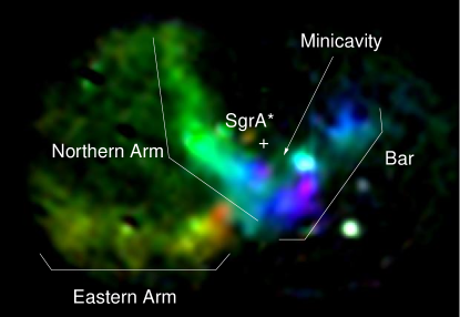
Figure 1: The Minispiral as seen by BEAR in Br$\gamma$$\,{}^{b}$. This picture is a composite of three images obtained from the BEAR cube through three virtual filters. The colours give therefore the velocity field of the Minispiral, from $-350\text{~{}km~{}s}^{-1}$ (red) to $+350\text{~{}km~{}s}^{-1}$ (purple). The standard names of some ISM features are given. A few emission line stars show up as point sources: GCIRS 16NE and 16C just east of Sgr A^⋆, The AF and AF NW stars below the Bar, and the GCIRS 13E cluster on the western edge of the Minicavity.

The first treatment to find the spectral features is to remove the continuum emission from the stars to obtain the line cubes. This can be done by linear interpolation between two neighbouring continuum regions if the cube contains only a narrow band (case of BEAR) or by fitting a simple function, like a polynomial, if the continuum is not nearly linear (case of SPIFFI). Once the stellar continuum is subtracted, the BEAR Br$\gamma$ data are dominated by the extended emission from the ionised ISM (Fig. 1 ). In Paumard et al. (2004), we have decomposed each spectrum in the field into several velocity components of the same line. Assuming that the ISM is made of clouds of finite velocity gradient material, we have decomposed the Minispiral into 9 components that are often superimposed on each other. In this paper, we have shown that these features are sufficiently thick to be responsible for a significant extinction, on the order of half of the K flux. This is consistent with the high spatial variability of $A_{V}$ in this region. This decomposition required the very high spectral resolution provided by BEAR, because the lines from two structures along the same line of sight are often very close to one another in the spectral domain. In some cases indeed, this spectral separation goes down to $0\text{~{}km~{}s}^{-1}$. In these cases, interpolation must be used to perform the decomposition using information from neighbouring points where the two structures are sufficiently separated.

These ISM features are really intermingled with the stellar content. It is therefore necessary to subtract the interstellar contribution in order to analyse this stellar population. In Paumard et al. (2001), updated in Paumard et al. (2003), we have again used both the high spectral resolution of BEAR and its spatial properties in the He i $\lambda$ $2.058\text{~{}}\mu\text{m}$ to discriminate between the stellar and interstellar lines, showing that some previous reports of Helium stars were indeed false, and due to insufficient correction of the extended emission. To clean the BEAR stellar spectra, we simply cut out the ISM lines manually. These lines were identified by visually exploring the cube and using the 2D information it contained. This simple correction was of good enough quality because at this very high resolution, the observed ISM line width ($\lesssim 20\text{~{}km~{}s}^{-1}$) was much smaller than the spectral scale of the stellar features ($\gtrsim 150\text{~{}km~{}s}^{-1}$). For these data, we had extracted the spectra of previously reported He-stars, and visually inspected the cube for more stars. We hence reported three new detections in the field, out of which one (N6) turned out to be essentially an unresolved thread of ionised ISM, the two others being now confirmed by SPIFFI.

The SPIFFI data lack the spectral resolution required to clean each individual spectrum of the narrow ISM lines it contains, but the spatial resolution is so high (and it will still improve with the upcoming adaptive optics system) that it is now possible to reliably estimate the extended line emission component by interpolating each frame of the cube over the locations of the point line emission or absorption sources. More specifically, the steps that have been applied for this correction are the following: (1) determination of the CO index (a measure of the depth of the $2.3\text{~{}}\mu\text{m}$ CO absorption band) of each star using narrow-band NACO images; (2) the stars with a low CO index are suspected early-type stars; (3) for each spectral channel of the line cube (i.e. continuum subtracted), an aperture corresponding to each possible early-type star is marked as unavailable data; (4) each frame of the line cube is interpolated over these unavailable regions; (5) a low spatial-frequency pass filter is applied to each frame, the cube resulting from these steps is the ISM cube, it normally contains only the ISM emission plus most of the noise; (6) this ISM cube is then subtracted from both the original cube and the line cube to obtain the stellar cube and stellar line cube, out of which a spectrum for each suspected early-type star is extracted.

3.2 Identification of the featured stars

This leads to over 100 spectra, most of which actually show spectral signatures typical of early-type stars. However, at this point, it is not clear which feature really belongs to which star, as the spectrum of every star is contaminated by the wings of the neighbouring stars. The most straightforward way of resolving this degeneracy is visual inspection: for each feature of each spectrum, it is possible to extract from the stellar line cube an image integrated exactly over the spectral domain corresponding to the maximum emission (resp. absorption) of the given feature. In most cases, a local maximum (resp. minimum) appears on this image in the vicinity of the studied star. The exact location of this extremum reveals to which star the feature belongs, i.e., to the studied star or to one of its neighbours. This visual method is inappropriate for heavy duty work such as that implied by the analysis of the GC content, which, as already mentioned, contains hundreds of candidates and dozens of stars actually showing features accessible to SPIFFI. In particular, this method requires considerable interaction by the observer, and does not make use of the fact that a given early-type star should typically show more than one feature. Furthermore, the features do not have to be simple, the lines often show P Cygni profiles, or consist of several lines from different species, both in emission and absorption (for instance, a typical feature at $2.11\text{~{}}\mu\text{m}$ is made of two He i  lines, often in absorption, one of which is itself a doublet, and one N line, often in emission for O stars). It would therefore be more appropriate to use the entire spectra to determine the spatial location of the stars to which they belong.

Figure 2: Dashed spectrum: one of the original spectra (GCIRS 33N); dash-dotted: the corresponding ISM spectrum; solid: the corrected stellar spectrum.

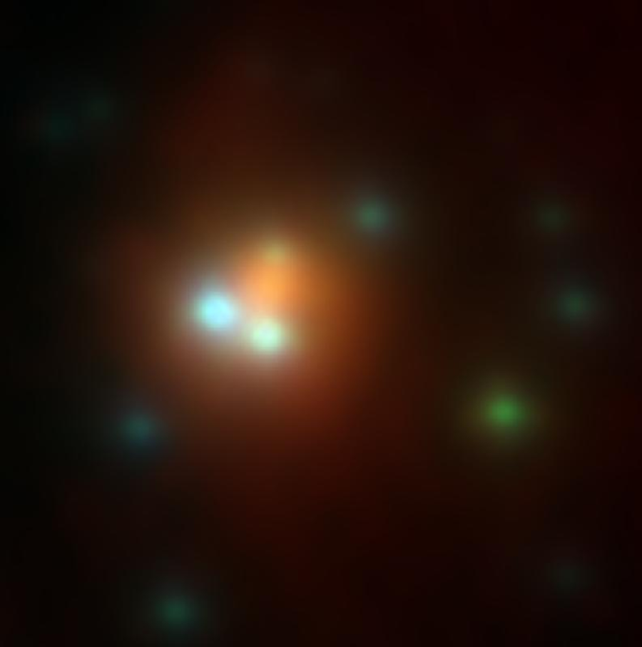
Figure 3: HK’L composite image of GCIRS 13E$\,{}^{b}$.

We have developed a method specifically to achieve this purpose. Each extracted stellar spectrum can be considered as a template that we want to compare with the individual spectra at each pixel of the field, in order to determine the point in the field from which this spectrum arises and spreads because of the spatial PSF. This comparison is done by means of correlation: for each template spectrum (each spectrum previously extracted from the stellar line cube), a correlation map is built. This map contains, for each pixel in the field, the correlation factor between the template and the spectrum contained in the stellar line cube at this location. This map normally contains a local maximum at the true location of the star to which the features of the template spectrum belong. This technique can easily be automated, and takes the entire continuum-subtracted spectrum of the stars into account. Furthermore, this technique can be generalised to provide both a complementary detection technique of the candidate early-type stars, and a first automated spectral classification of the stars. In the method described above, one can allow for a Doppler shift between the template spectrum and the spectra in the cube. This corresponds to tracing the maximum of the cross-correlation function for each spatial location rather simply using correlation. In that case, every other star in the field showing a spectrum similar to the template will show up as a local maximum on the map. It will therefore be possible to automatically determine which stars have a spectrum similar to the template.

When this cross-correlation work has been done, many candidates can be rejected, as they do not show detectable features. Other stars can be added to the list of candidates because they have been found on the cross-correlation map of one of the templates. The extraction procedure described above can then be iterated to take this information into account. This is necessary because information concerning the ISM emission should not be wasted by blanking out the region containing a candidate early-type star that has been shown indeed not to show detectable features; and on the contrary the features from the newly detected candidates must be cleared out as well as possible. This second extraction led to $29$ spectra, all of them showing recognisable features typical of early-type stars, and associated unambiguously with a single star (within the precision allowed by the spatial resolution of the instrument).

All the stars previously studied with BEAR within the field of SPIFFI are detected here as well. As already stated, object N6 from Paumard et al. (2001) does not correspond to an He star but to a tiny ISM feature; however, this ISM feature coincides in projection, and may be physically associated, with four stars that indeed show some He feature (ID 24, 26, 31 and 33). Furthermore, for the first time, thanks to their high spatial resolution as well as high signal-to-noise ratio, these SPIFFI data allow detection of faint emission lines as well as absorption lines, which are totally filled by ISM emission on the raw data. Fig. 3 shows one of the original spectra, the ISM profile determined as in Sect. 1, and the inferred stellar spectrum. After correction for the very intense interstellar Br$\gamma$ line, a complex stellar feature made of Br$\gamma$ and He i in absorption appears.

4 GCIRS 13E: a case for spectro-imaging

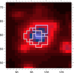
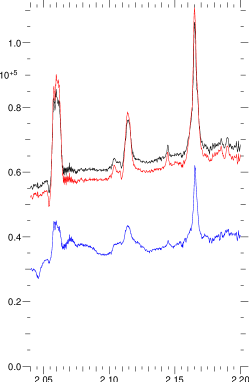
a)  b)  c)

Figure 4: SPIFFI spectra of GCIRS 13E: a) apertures used, b) raw (blended) spectra, c) final object spectra.

Among these objects, GCIRS 13E deserves special attention. This source is bright at all wavelength from sub-mm to X rays. A three colour high-resolution image (Fig. 3) made from Gemini H and K’ and ESO 3.6m L band data illustrates that it contains three blue stars and a very red core. Deconvolution of these three images plus narrow band NICMOS images (Maillard et al., 2004) has shown that GCIRS 13E is indeed a cluster of at least seven evolved massive stars: even the three red objects at the cluster core can be interpreted as dusty Wolf-Rayets. $A_{V}$ can be derived from the two assumptions that it does not vary significantly within the cluster and that the bluest star is in the Rayleigh-Jeans regime ($T_{\text{eff}}\gtrsim 25\,000$ K at this wavelength), which is proven by the fact that two of the stars show emission in a NICMOS Pa$\alpha$  image. This multi-wavelength, high spatial resolution study can be considered as a kind of low spectral resolution attempt. However, the exact spectral type of these hot stars cannot be unambiguously established by this technique, because more spectroscopic information is needed. Therefore, spectra of the individual components are required to achieve this purpose.

The sources are too close to one another to allow for individual aperture spectroscopy. Any attempt to do this is doomed to give spectra significantly affected by one another. In Fig. 4, we show three spectra obtained from the SPIFFI data through three overlapping virtual apertures; two of them seem identical, whereas the third is clearly affected by a blend with these. Reducing these apertures would reduce the signal-to-noise ratio while not providing much better results. However, the spectrum obtained through each of the apertures is a linear combination of the spectra of all the stars (at least seven indeed). It is therefore possible to obtain three independent spectra by linear combination of these three observed spectra, leading to spectra typical of three of the types discussed below (Fig. 4c), although it is not yet clear whether the upper spectrum in this figure belongs to the blue star north of the cluster or to the red stars in the middle.

5 The (known) stellar population of early-type stars

Table 1: Translation of ID numbers in the figures to common names. Offsets from Sgr A^⋆ (RA, dec. in arcsec) are given for so far anonymous stars.

Fig. 6	Fig. 6	Name
N1	41	IRS 16NE
N2	14	IRS 16C
N3	17	IRS 16SW
N4	13	IRS 16NW
N5	48	IRS 33SE
N7	75	IRS 34W
B1		ID 180a
B2		IRS 7E2
B3	178	IRS 9W
B4		IRS 15SW
B5	61	IRS 13E2
B6		IRS 7W
B7		AF star

Fig. 6	Fig. 6	Name
B8		AF NW
B9		HeIN3
B10		BSD WC9
B11	27	IRS 29N
B12		IRS 15NE
B13	46	IRS 16SE2
	1	S2 (S0-2)
	7	S1-3
	23	IRS 16CC
	24	$1.447$, $-1.49$
	26	$1.593$, $-1.355$
	31	IRS 16SE1
	32	IRS 33N

Fig. 6	Name
33	MPE 1.6-6.8
34	IRS 29NE1
53	IRS 13E1
57	IRS 13E northb
72	$0.774$, $-4.047$
81	IRS 34NW
87	IRS 1W
97	$3.195$, $-4.842$
110	$6.372$, $0.227$
179	$1.8$, $-6.3$
180	IRS 3c
181	$0.665$, $-1.608$

$a$: in Ott et al. (1999); $b$: north of the cluster, exact identification uncertain; $c$: the emission line star is offset by about $0.1^{\prime\prime}$ from the bright K-band source.

The main results obtained with BEAR (Paumard et al., 2001, 2003) are that the He stars can indeed be classified in two groups, from their line width (mean $\text{FWHM}\simeq 225\pm 75\text{~{}km~{}s}^{-1}$ for the narrow line stars and $1025\pm 400\text{~{}km~{}s}^{-1}$ for the broad line stars) and K magnitude: all the narrow line stars are more luminous than the broad line stars, by more than $2$ magnitudes in average (in Paumard et al. 2001, we reported that one narrow line star, GCIRS 34W, was less luminous than the others, but that was due to a temporary obscuration event, as discussed in Paumard et al. 2003 and below). A third, striking property of these two stellar classes is their spatial distribution (Fig. 6): the narrow line stars are concentrated in the GCIRS 16 complex, whereas the broad line stars are distributed in the entire field. Table 1 gives the translation between the identification numbers used in Fig. 6, in Figs. 6 to 12, and common names.

The SPIFFI data set that we have analysed so far has a smaller field, and therefore does not add much information on these two different spatial distributions. However, thanks to their other characteristics already discussed (wide band, high spatial resolution, and high signal-to-noise ratio), they give a lot of interesting results. We will hereafter present the spectra of all the early-type stars that we have found, together with a discussion of their data type. The spectra presented here are limited to the range $2.04-2.20\text{~{}}\mu\text{m}$, for comparison with Hanson et al. (1996). The reduction software being still under heavy development, some artifacts remain, which take the form of strong noise spikes. The spectra are given in Figs. 9 to 12, and their spatial distribution is given in Fig. 6. The various vertical lines on Figs. 9 to 12 mark several atomic lines: green: He i, pink: carbon, red: H (Br$\gamma$), blue: He ii.

Early Wolf-Rayet stars:

Figure 5: Spatial distribution of the narrow (N) and broad (B) line stars.

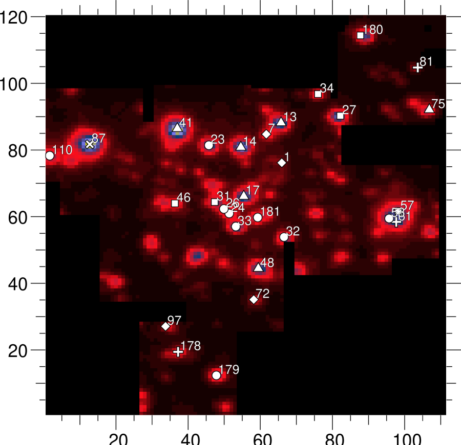
Figure 6: Spatial distribution of the 6 stellar types: early (squares) and late (vertical crosses) Wolf-Rayet stars, LBVs (triangles), OBN stars (circles), a candidate Be star (diagonal cross), and a few more OB stars.

Six stars show very broad features mainly from C iv and/or N; they are early Wolf-Rayet stars (WC and WNE). Some of them also show some Br$\gamma$ emission. GCIRS 16SE2 had been mistaken for a broad He i emission line star in Paumard et al. (2003). This was due to the fact that an unidentified absorption feature at roughly $2.045\text{~{}}\mu\text{m}$ lays in our short wavelength continuum region, which mimicked a low signal-to-noise, broad emission line on a very red continuum. GCIRS 29N shows broad and tenuous features of C iv and N, but also He i; it was the broad He i-line stars B11 in Paumard et al. (2003) and may be of a slightly later type than the other stars of this group. Its weak He i $\lambda$ $2.058\text{~{}}\mu\text{m}$ resembles that of the star Blum WC9 (B10), which could therefore be of the same type. These seven stars are randomly spread over the entire field.

Late Wolf-Rayets: The second subset of stars is typical of late Wolf-Rayet stars (WNLs), with rather broad and bright He i, He ii, Br$\gamma$ and N lines. Two of them show a broad He i $\lambda$ $2.058\text{~{}}\mu\text{m}$ line, typical of the broad-line He-stars discussed in Sect. 5. All these broad-line stars (except B10, B11 and B13 already discussed) therefore seem to be WNLs as well.

Luminous Blue Variables:

Figure 7: Early Wolf-Rayets.

Figure 8: Late Wolf-Rayets.

Figure 9: Luminous Blue Variables.

The third subset corresponds exactly to the narrow-line stars discussed in Sect. 5. In this wavelength domain, they are characterised by their rather strong, narrow He i $\lambda$ $2.058\text{~{}}\mu\text{m}$ line with a clear P Cyg profile; an equally strong feature at $2.166\text{~{}}\mu\text{m}$ made mainly of Br$\gamma$ as well as a clear contribution of He i $\lambda$ $2.163\text{~{}}\mu\text{m}$; this complex does not show a P Cyg profile, but that may be mainly because of the blending; a complex of He i (in absorption for all but one star) and N (in emission) around $2.11\text{~{}}\mu\text{m}$. These spectra are typical of so called “transitory” stars, Ofpe/WN9 and Luminous Blue Variables (LBVs). Morris et al. (1996) seems to show that all these types may relate to objects of the same nature, maybe in different states. As already stated these stars are all within the GCIRS 16 cluster. GCIRS 34W deserves special attention: this is the only one to have already shown an obscuration event, which fully qualifies it as an LBV; this is the only one that shows the He i $\lambda$ $2.11\text{~{}}\mu\text{m}$ complex in emission; and this is the star for which the spatial association with the GCIRS 16 cluster is the most controversial. The first point above does not mean that the other stars are not LBVs as well, as obscuration events of LBV stars are indeed rare (Humphreys et al., 1999). Neither does the second, as the spectra of LBVs are variable as well as their luminosity: the fact that the He i $\lambda$ $2.11\text{~{}}\mu\text{m}$ complex of GCIRS 34W is currently in emission could be related to its obscuration event.

OBN stars:

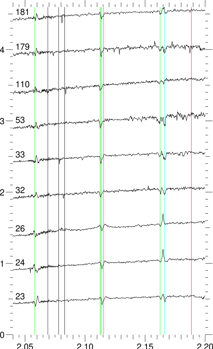
Figure 10: N- and He-rich stars (OBN).

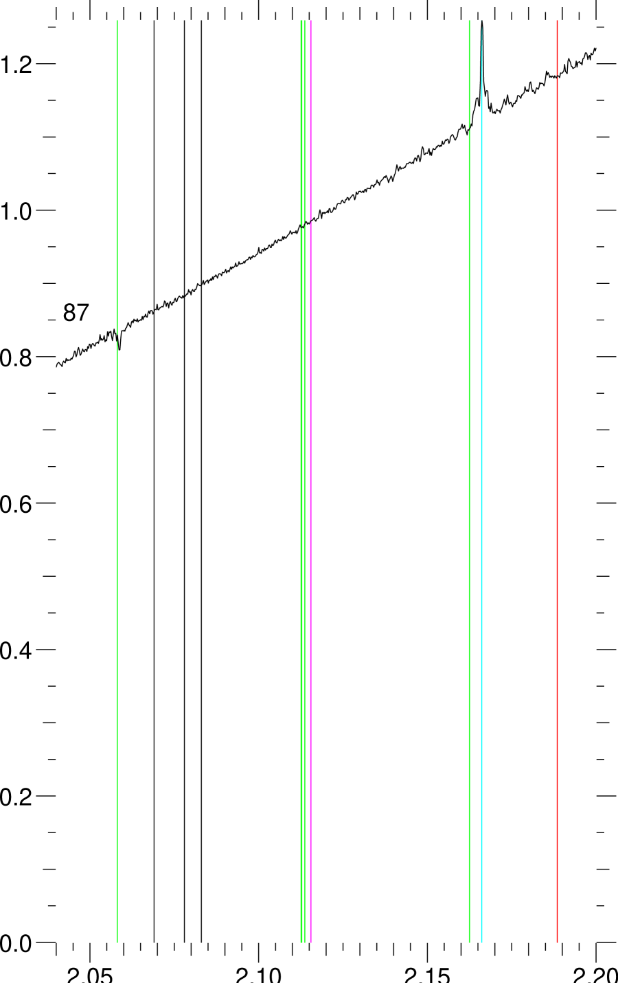
Figure 11: GCIRS 1W, a candidate Be star.

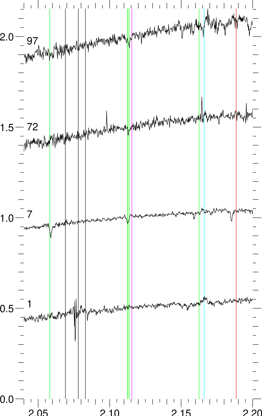
Figure 12: More OB stars.

The third type is defined by stars which show: He i $\lambda$ $2.058\text{~{}}\mu\text{m}$ (often with a complex structure); the He i $\lambda$ $2.11\text{~{}}\mu\text{m}$ complex in absorption; often N $\lambda$ $2.11\text{~{}}\mu\text{m}$ in emission; comparable Br$\gamma$ and He i $\lambda$ $2.163\text{~{}}\mu\text{m}$, mostly in absorption, but sometimes with some emission in-between. Note that the three stars that show emission at $2.166\text{~{}}\mu\text{m}$ are in a crowded area, and two of them are superimposed upon a very compact thread of ISM material. The ISM correction at this very location is therefore somewhat suspicious. We had reported a He star at this location with BEAR, but the same comment applies to this detection as well.

Following the independent stellar classification scheme in the K-band (hence the “k” prefix) by Hanson et al. (1996), these stars can be classified in various kOB subtypes (kOBh+, kOBh-, kO7-O8, kO9-B1b+, kOBb and kOBbh+). It is hard to give an unambiguous classification in the MK system for these stars, for two reasons: a unambiguous relationship between the MK system and the K band classification scheme by Hanson et al. (1996) does fundamentally not seem to exist; and very few standard stars have been studied so far both in the optical and infrared to provide ground for comparison. This is particularly true for OB stars.

However, when one compares directly these stars to the templates shown in Hanson et al. (1996), it appears clearly that only two stars exhibit a similar feature at $2.166\text{~{}}\mu\text{m}$, with comparable Br$\gamma$ and He i: HD 191781 (kOBbh+) and HD 123008 (kO7-O8bh-). Both are ON9.7 supergiants. ON and BN stars (generically called OBN stars) are particular kinds of O and B stars which show unusual N lines in the optical. They are also known to show unusually strong He lines, and to be particularly bright because of a lower atmospheric opacity (Langer, 1992). Indeed, our 9 stars are particularly bright, as a typical O9 supergiant should be at most 1.4 magnitudes brighter than S2 (a O8-B0V star according to Ghez et al. 2003, of $m_{K}=13.95$), whereas their K magnitudes span the 10.43–12.63 range. It therefore seems likely that these nine stars are indeed N- and He-rich stars that would appear in the optical as OBN stars.

GCIRS 1W: a Be star? GCIRS 1W is known to exhibit a very flat and very red spectrum, to be embedded within the Northern Arm and to interact with it to form a bow shock (Tanner et al., 2004). Study of this star is made difficult by the fact that it is a local source of excitation for the ISM, and is therefore coincident with a local maximum of the ionised gas emission. However, the correction described in Sect. 3.1 allows us to unambiguously identify the He i $\lambda$ $2.06\text{~{}}\mu\text{m}$ line in absorption as well as the Br$\gamma$ line in emission. This spectrum is similar to that of the Be star DM +49 3718 in Hanson et al. (1996). Indeed, all the stars in this atlas which show Br$\gamma$ in emission and no He i $\lambda$ $2.11\text{~{}}\mu\text{m}$ are Oe or Be stars.

More OB stars: Finally, a few more stars exhibit at least one He i line or the Br$\gamma$ line. Star number 1 (S2) shows only to a detectable level the Br$\gamma$ line, and we are mostly able to detect it because a very high Doppler shift (about $1400\text{~{}km~{}s}^{-1}$) puts it away from the ISM residuals, at about $2.155\text{~{}}\mu\text{m}$. This star and others of its kind will be more easily studied when SPIFFI is equipped with adaptive optics. The three other stars show mostly the He i $\lambda$ $2.163\text{~{}}\mu\text{m}$ line. The absence of detection of Br$\gamma$ is certainly due to the noise in that region of the spectrum, which comes from the residuals of the ISM feature.

6 Formation scenarios

The existence of the early-type stars at their current position can basically be explained in two ways: either they have been formed in situ, or they have been formed somewhere else in the Galaxy before they have been drawn here. Various items in the literature argue that gravitational collapse of a gas cloud is prevented in the tidal field of Sgr A^⋆, and that therefore star formation cannot have occurred in situ. However, Levin & Beloborodov (2003) show that stellar formation in the vicinity of a SMBH is likely to occur if the black hole possesses a massive enough accretion disk. This consideration transforms the problem into: did Sgr A^⋆ possess a massive, parsec scale accretion disk $10^{6}$ years ago? The fact is that Sgr A^⋆ does not appear to possess a disk, of any observable scale, right now. The ISM that can be seen at the parsec scale is concentrated in the CND (which may contain about $10^{4}\text{~{}M}_{\odot}$ of material, Christopher & Scoville 2003) and in the Minispiral, for which $10^{3}\text{~{}M}_{\odot}$ seems to be a reasonable upper limit, as the estimates for two of the nine components of the Minispiral are $\simeq 10\text{~{}M}_{\odot}$ (Liszt, 2003; Paumard et al., 2004). However, Morris et al. (1999) show that current absence of a disk remains compatible with in situ formation within an accretion disk in the context of a limit cycle.

The other possibility is that these stars have been formed at some distance, and then moved into the central parsec. The presence of the Arches and Quintuplet clusters at a distance of about $35$ pc shows that massive star cluster formation is indeed possible at these distances. According to McMillan & Portegies Zwart (2003), a cluster with a dense enough core ($\gtrsim 10^{5}\text{~{}M}_{\odot}$), formed within $20$ pc, could spiral down to the central parsec within the lifetime of the most massive stars. It would however be stripped during its cruise, so that it would eventually deposit only a small fraction of its mass into the central region. However, it is not yet clear whether this scenario could explain the stars closest to Sgr A^⋆, at only a few light days, and Kim & Morris (2003) and Kim et al. (2004) conclude that they are unable to find realistic initial conditions to their simulations that would lead to the observed situation through infall of a cluster.

These two possibilities should lead to somewhat different clusters in the end: for instance, the spiralling-in cluster scenario probably predicts that a significant number of young stars of all masses, co-eval with the inner parsec early-type stars, should be found in the few central tens of parsecs, as a byproduct of the stripping of the infalling cluster. Such a population is not yet known. Actually observing it would require at least deep imaging in the J, H and K bands, at the best available resolution and over a field of about $3\times 3$ arcmin².

The observed properties of the early-type stars that need to be addressed are the following: a group of 15 N- and He-rich stars (the LBVs and the ON stars) are seen within a small region (about $5^{\prime\prime}$ or one light-year), offset from Sgr A^⋆ by about $1^{\prime\prime}$; there are about two dozen Wolf-Rayet stars dispersed apparently randomly (in projection) in the central few parsecs; and there is a compact cluster of evolved stars (GCIRS 13E), that contains members of both the above-mentioned groups of stars. These properties can be classified in two types: first, the spatial distribution of the stars, and second their spectral types. The actual spatial distribution is clearly subject to caution as we only have access to a projected distribution. However, at least two velocity components are available for all the stars within the central two parsecs, and a radial velocity is also being obtained for a growing number of them: these four to five dimensions should be enough to constrain the dynamical models. An important point in the spatial distribution is that several groups of stars are observed. One of the groups, GCIRS 13E, is a compact cluster. It is proposed in Maillard et al. (2004) that this could be the remaining core of an infalling cluster. However, it must be asked whether such a compact cluster could itself form in situ.

Concerning the spectral types, the fact reported here that more stars within the GCIRS 16 cluster are N- and He-rich should also be addressed by the models. These kinds of stars have experienced an unusual mixing. It can be the trace of a fast initial rotation of the proto-stars, that would be due to the initial conditions. It may be explained by the shear if the stars have been formed within an accretion disk. The efficient mixing within the GCIRS 16 stars could also come from close-by interactions with Sgr A^⋆, but it would be hard to explain how these stars can be seen know as an offset group, rather than a spheroidal cluster centred on Sgr A^⋆.

7 Conclusion

Spectro-imaging techniques have been applied to the GC, providing very valuable information on the nature of the early-type stars lying there, and on their spatial distribution. Upcoming commissioning of the adaptive optics system that will be used in conjunction with SPIFFI must be anticipated to give even more spectacular results. These stars appear to belong to several segregated groups, distinct in their spatial distribution and stellar types, but not apparently in their age. One of these groups is made of moderately evolved stars that show core-processed material at their photosphere, which is not exceptional, but unusual. The more evolved stars, already at the WR stage, have probably lost any spectral signature that would have shown whether they were already N- and He-rich before they reached this stage. All these observations are far from trivial and should give strong constraints on the formation scenarios.

References

- Blum et al. (1996) Blum, R. D., Sellgren, K., & Depoy, D. L. 1996, ApJ, 470, 864
- Christopher & Scoville (2003) Christopher, M. H. & Scoville, N. Z. 2003, in ASP Conf. Ser. 290: Active Galactic Nuclei: From Central Engine to Host Galaxy, 389
- Eisenhauer et al. (2003) Eisenhauer, F., Abuter, R., Bickert, K., et al. 2003, in Instrument Design and Performance for Optical/Infrared Ground-based Telescopes, ed. Masanori Iye & Alan F. Moorwood, Proc. SPIE, 4841, 1548
- Eisenhauer et al. (2000) Eisenhauer, F., Tecza, M., Mengel, S., et al. 2000, in Optical and IR Telescope Instrumentation and Detectors, ed. Masanori Iye & Alan F. Moorwood, Proc. SPIE, 4008, 289
- Ghez et al. (2003) Ghez, A. M., Duchêne, G., Matthews, K., et al. 2003, ApJ, 586, L127
- Ghez et al. (2004) Ghez, A. M., Salim, S., Hornstein, S. D., et al. 2004, ApJ, submitted, astro-ph/0306130
- Hanson et al. (1996) Hanson, M. M., Conti, P. S., & Rieke, M. J. 1996, ApJS, 107, 281
- Humphreys et al. (1999) Humphreys, R. M., Davidson, K., & Smith, N. 1999, PASP, 111, 1124
- Kim et al. (2004) Kim, S. S., Figer, D. F., & Morris, M. 2004, ApJ, 607, L123
- Kim & Morris (2003) Kim, S. S. & Morris, M. 2003, ApJ, 597, 312
- Krabbe et al. (1995) Krabbe, A., Genzel, R., Eckart, A., et al. 1995, ApJ, 447, L95
- Langer (1992) Langer, N. 1992, A&A, 265, L17
- Levin & Beloborodov (2003) Levin, Y. & Beloborodov, A. 2003, ApJ, 590, L33
- Liszt (2003) Liszt, H. S. 2003, A&A, 408, 1009
- Maillard et al. (2004) Maillard, J. P., Paumard, T., Stolovy, S. R., & Rigaut, F. 2004, A&A, accepted, astro-ph/0404450
- McMillan & Portegies Zwart (2003) McMillan, S. L. W. & Portegies Zwart, S. F. 2003, ApJ, 596, 314
- Morris et al. (1999) Morris, M., Ghez, A. M., & Becklin, E. E. 1999, Advances in Space Research, 23, 959
- Morris et al. (1996) Morris, P. W., Eenens, P. R. J., Hanson, M. M., Conti, P. S., & Blum, R. D. 1996, ApJ, 470, 597
- Ott et al. (1999) Ott, T., Eckart, A., & Genzel, R. 1999, ApJ, 523, 248
- Paumard et al. (2004) Paumard, T., Maillard, J. P., & Morris, M. 2004, A&A, accepted, astro-ph/0405197
- Paumard et al. (2001) Paumard, T., Maillard, J. P., Morris, M., & Rigaut, F. 2001, A&A, 366, 466
- Paumard et al. (2003) Paumard, T., Maillard, J. P., & Stolovy, S. R. 2003, in Galactic Center Workshop 2002: The Central 300 parsecs, ed. A. Cotera, S. Markoff, T. R. Geballe & H. Falcke, Astron. Nachr., 324 S1/2003, 303
- Schödel et al. (2003) Schödel, R., Ott, T., Genzel, R., et al. 2003, ApJ, 596, 1015
- Tanner et al. (2004) Tanner, A., Ghez, A., & Morris, M. 2004, ApJ, submitted
- Thatte et al. (1998) Thatte, N. A., Tecza, M., Eisenhauer, F., et al. 1998, in Adaptive Optical System Technologies, ed. Domenico Bonaccini & Robert K. Tyson, Proc. SPIE, 3353, 704