Implications of the Measured Image Size for the Radio Afterglow of GRB 030329

Abstract

We use data on the image size of the radio afterglow of GRB 030329 (Taylor et al. 2004) to constrain the physical parameters of this explosion. Together with the observed broad band spectrum, this data over-constrains the physical parameters, thus enabling to test different GRB jet models for consistency. We consider two extreme models for the lateral spreading of the jet: model 1 with relativistic expansion in the local rest frame, and model 2 with little lateral expansion as long as the jet is highly relativistic. We find that both models are consistent with the data for a uniform external medium, while for a stellar wind environment model 1 is consistent with the data but model 2 is disfavored by the data. Our derivations can be used to place tighter constraints on the dynamics and structure of GRB jets in future afterglows, following a denser monitoring campaign for the temporal evolution of their image size.

1. Introduction

It has long been recognized that direct imaging of Gamma-Ray Bursts (GRBs) can provide important constraints on their physical parameters (Waxman, 1997; Sari, 1998; Panaitescu & Mészáros, 1998; Granot, Piran & Sari, 1999a, b; Granot & Loeb, 2001). Unfortunately, the characteristic size of a GRB image is only of order a micro-arcsecond about a day after the GRB at the Hubble distance, and so it cannot be resolved by existing telescopes. Nevertheless, indirect constraints on the image size of GRB afterglows were derived based on the transition between diffractive and refractive scintillations (Goodman, 1997) in the radio afterglow of GRB 970508 (Frail et al., 1997; Waxman, Kulkarni & Frail, 1998), and based on microlensing by a star in a foreground galaxy (Loeb & Perna, 1998) for the optical lightcurve of GRB 000301C (Garnavich, Loeb & Stanek, 2000; Granot & Loeb, 2001; Gaudi & Loeb, 2001; Mao & Loeb, 2001; Gaudi, Granot, & Loeb, 2001).

Obviously the challenge of imaging a GRB is made easier for nearby sources where the late radio afterglow extends over a wide, possibly resolvable angle (Woods & Loeb, 1999; Cen, 1999; Wang & Loeb, 2001; Paczyński, 2001; Granot & Loeb, 2003). Recently, Taylor et al. (2004) have used a VLBI campaign to measure, for the first time, the angular size and proper motion of the radio afterglow image of the bright, nearby ($z=0.1685$) GRB 030329. The diameter of the afterglow image was observed to be $\sim 0.07\;$mas (0.2 pc) after 25 days and $0.17\;$mas ($0.5\;$pc) after 83 days, indicating an average velocity of $\sim 4.1-5.7\;$c. This superluminal expansion is consistent with expectations of the standard relativistic jet model (Oren, Nakar & Piran, 2004). The projected proper motion of GRB 030329 was measured to be smaller than 0.3 mas for 80 days following the GRB.

Here we use the data of Taylor et al. (2004) to constrain the physical parameters of GRB 030329 based on detailed modelling of the collimated relativistic hydrodynamics of GRB afterglows. Since the current state-of-the-art modelling of afterglow jets is still flawed with uncertainties (Rhoads, 1999; Sari, Piran & Halpern, 1999; Granot et al., 2001; Kumar & Granot, 2003; Salmonson, 2003; Cannizzo, Gehrels & Vishniac, 2004), we use this data to critically assess some classes of models that were proposed in the literature. An important difference between relativistic radio jets of GRBs and the better-studied relativistic radio jets of quasars (Begelman, Blandford & Rees, 1984) or micro-quasars (Mirabel & Rodríguez, 1999) is that active quasars often inject energy over extended periods of time into the jet while GRB sources are impulsive. Although quasar jets remain highly collimated throughout their lifetimes, GRB jets decelerate and expand significantly once they become non-relativistic, $\sim 1\;$yr after the explosion. The hydrodynamic remnant of a GRB eventually becomes nearly spherical only after $\sim 5\times 10^{3}\;$yr (Ayal & Piran, 2001).

The outline of the paper is as follows. In §2, we discuss the expected image size of radio afterglows and its relation to the observed flux density below the self absorption frequency. In §3, we analyze the expected temporal evolution of the afterglow image size. The expected linear polarization is discussed in §4, while the surface brightness profile across the image and its effects on the estimated source size are considered in §5. Finally, we apply these derivations to the radio data of GRB 030329 (§6) and infer the physical parameters from the measured spectrum (§7). We conclude in §8 with a discussion of our primary results and their implications.

2. The Image Size and Synchrotron Self Absorption

In GRB afterglows, relativistic electrons are accelerated in the advancing shock wave to a power law distribution of energies, $dN/d\gamma_{e}\propto\gamma_{e}^{-p}$ for $\gamma_{e}\geq\gamma_{m}$. For $p>2$, the minimal Lorentz factor of the electrons is given by

$$\gamma_{m}=\left(\frac{p-2}{p-1}\right)\frac{m_{p}}{m_{e}}\,\epsilon_{e}(\Gamma-1)\ ,$$ (1)

where $\epsilon_{e}$ is the fraction of the internal energy behind the shock in relativistic electrons, and $\Gamma$ is the bulk Lorentz factor of the shocked fluid. There is a spectral break at $\nu_{m}=\nu_{\rm syn}(\gamma_{m})$, the synchrotron frequency of electrons with $\gamma_{e}=\gamma_{m}$. Another break in the spectrum occurs at $\nu_{c}=\nu_{\rm syn}(\gamma_{c})$, the synchrotron frequency of an electron that cools on the dynamical time.

At sufficiently low frequencies, below the self absorption frequency $\nu_{sa}$, the optical depth to synchrotron self absorption $\tau_{\nu}$ becomes larger than unity, causing an additional break in the spectrum. In this spectral range, the emitted intensity is given by the Rayleigh-Jeans part of a black body spectrum, where the black body temperature is taken as the effective temperature $T_{\rm eff}$ of the electrons that are emitting the radiation at the observed frequency $\nu$. In the local rest frame of the emitting fluid this may be written as

$$I^{\prime}_{\nu^{\prime}}=\frac{2(\nu^{\prime})^{2}}{c^{2}}k_{B}T_{\rm eff}=\frac{2(\nu^{\prime})^{2}}{c^{2}}\gamma_{\rm eff}m_{e}c^{2}\ ,$$ (2)

where primed quantities are measured in the local rest frame of the emitting fluid while un-primed quantities are measured in the observer frame (the rest frame of the central source). When $\nu_{sa}>\nu_{m}$, the emission at $\nu_{m}<\nu<\nu_{sa}$ is dominated by electrons for which $\nu\sim\nu_{\rm syn}(\gamma_{e})\propto\gamma_{e}^{2}$, giving $\gamma_{\rm eff}\propto\nu^{1/2}$ and $F_{\nu}\propto I_{\nu}\propto\nu^{5/2}$. For $\nu_{m}>\nu_{c}$ there is rapid cooling and all the electrons cool significantly within a dynamical time (Sari, Piran & Narayan, 1998). When $\nu_{m}>\max(\nu_{c},\nu_{sa})$, then as $\nu$ decreases below $\nu_{sa}$ the distance $l$ behind the shock where $\tau_{\nu}(l)=1$ decreases. The electrons in that location, which are responsible for most of the observed emission, have had less time to cool after passing the shock and therefore have a higher $T_{\rm eff}=\gamma_{\rm eff}(m_{e}c^{2}/k_{B})$. In this case $\gamma_{\rm eff}\propto 1/l\propto\nu^{-5/8}$ and $F_{\nu}\propto\nu^{11/8}$ (Granot, Piran & Sari, 2000). At a sufficiently small distance behind the shock, smaller than $l_{c}$, an electron with an initial Lorentz factor $\gamma_{m}$ does not have enough time to cool significantly after crossing the shock. Therefore, most electrons within a distance of $l_{c}$ from the shock have $\gamma_{e}\sim\gamma_{m}$, and the effective temperature in this region is $T_{\rm eff}\approx\gamma_{m}m_{e}c^{2}/k_{B}$. At sufficiently low frequencies (below $\nu_{ac}$, see Granot, Piran & Sari, 2000) $l$ becomes smaller than $l_{c}$ and $\gamma_{\rm eff}\approx\gamma_{m}$ independent of $\nu$, and therefore $F_{\nu}\propto\nu^{2}$ at $\nu<\nu_{ac}$. For slow cooling ($\nu_{m}<\nu_{c}$), $\gamma_{\rm eff}\approx\gamma_{m}$ and $F_{\nu}\propto\nu^{2}$ immediately below $\nu_{sa}$.

The observed specific intensity is given by $I_{\nu}=(\nu/\nu^{\prime})^{3}I^{\prime}_{\nu^{\prime}}$ and $\nu^{\prime}/\nu=(1+z)\Gamma(1-\beta\cos\theta)\sim(1+z)/\Gamma$ where $z$ is the source redshift and $\theta$ is the angle between the direction to the observer and the velocity vector of the emitting material in the observer frame. The observed flux density is $F_{\nu}=\int d\Omega\cos\tilde{\theta}I_{\nu}\approx\Omega I_{\nu}$ where $\Omega\approx\pi(R_{\perp}/D_{A})^{2}=(1+z)^{2}\pi(R_{\perp}/D_{p})^{2}=(1+z)^{4}\pi(R_{\perp}/D_{L})^{2}$ and $\tilde{\theta}\cong\tan\tilde{\theta}=R_{\perp}/D_{A}\ll 1$ are the solid angle and angular radius of the source image, respectively. Here $R_{\perp}$ is the radius of the observed image (its apparent size on the plane of the sky) and $D_{A}$, $D_{p}$ and $D_{L}$ are the angular, proper and luminosity distances to the source, respectively. Thus one obtains $I_{\nu}\approx[\Gamma/(1+z)]^{3}[2(\nu^{\prime})^{2}/c^{2}]kT_{\rm eff}\approx[\Gamma/(1+z)]2\nu^{2}\gamma_{\rm eff}m_{e}$, and (Katz & Piran, 1997)

$$F_{\nu}\approx 2\pi\nu^{2}m_{e}\Gamma\gamma_{\rm eff}(1+z)\left(\frac{R_{\perp}}{D_{p}}\right)^{2}\ .$$ (3)

In deriving Eq. (3) the specific intensity $I_{\nu}$ was assumed to be uniform across the observed image. A more accurate calculation would have to integrate over the contribution to the observed emission from different radii $R$ and angles $\theta$ from the line-of-sight for a fixed observed time $t$ (e.g., Granot, Piran & Sari, 1999b), which results in a non-uniform $I_{\nu}$ across the image. Therefore, when using Eq. (3) one must choose some effective value for $I_{\nu}$ which should correspond to its average value across the image. Since $I_{\nu}$ depends on $\Gamma$, this is equivalent to choosing an effective value of $\Gamma$. Since $\Gamma$ depends on $R$, one also has to find at which $R$ or $\theta$ should the value of $\Gamma$ be evaluated in Eqs. (1) and (3). Usually $\nu_{sa}<\nu_{m}<\nu_{c}$ in which case $\gamma_{\rm eff}\approx\gamma_{m}$ so that $I_{\nu}$ depends on $\Gamma$ not only through the Lorentz transformations, but also through the value of $\gamma_{m}$, i.e. $\Gamma$ enters into both Eqs. (1) and (3). Comparing Eq. (3) with the more accurate expression calculated by Granot & Sari (2002) using the Blandford-McKee (1976) self similar spherical solution, we find that the two expressions are in relatively good agreement if $\Gamma$ is evaluated just behind the shock at the location where $R_{\perp}$ is located. This should be a good approximation before the jet break time in the light curve,

$$t_{j} = \frac{(1+z)}{4c}\left[\frac{(3-k)E}{2\pi Ac^{2}}\right]^{1/(3-k)}\theta_{0}^{2}$$

$$\approx \left\{\begin{matrix}0.66(1+z)(E_{51}/n_{0})^{1/3}(\theta_{0}/0.1)^{2}\;{\rm days}&\ \ (k=0)\cr&\cr 0.34(1+z)(E_{51}/A_{*})(\theta_{0}/0.1)^{2}\;{\rm days}&\ \ (k=2)\end{matrix}\right.\ .$$

At $t>t_{j}$, however, it is less clear how well this approximation holds, and it might be necessary to evaluate $\Gamma$ at a different location. In particular, as we shall see below, this approximation does not work well for model 2 with $k=0$ where $\Gamma$ need to be evaluated near the head of the jet, rather than at the side of the jet where $R_{\perp}$ is located.

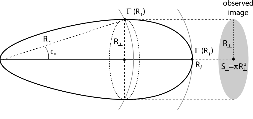
Figure 1.— Schematic illustration of the equal-arrival time surface (thick black line), namely the surface from where the photons emitted by the shock front arrive at the same time to the observer (far on the right-hand-side). The maximal lateral extent of the observed image, $R_{\perp}$, is located at an angle $\theta_{*}$, where the shock radius and Lorentz factor are $R_{*}$ and $\Gamma_{*}=\Gamma_{\rm sh}(R_{*})$, respectively. The area of the image on the plane of the sky is $S_{\perp}=\pi R_{\perp}^{2}$. The shock Lorentz factor $\Gamma_{\rm sh}$ varies with $R$ and $\theta$ along the equal-arrival time surface. The maximal radius, $R_{l}$, on the equal-arrival time surface is located along the line-of-sight. If, as expected, $\Gamma_{\rm sh}$ decreases with $R$, then $\Gamma_{l}=\Gamma_{\rm sh}(R_{l})$ is the minimal shock Lorentz factor on the equal-arrival time surface.

The image size is given by $R_{\perp}=\max(R\sin\theta)$ along the equal arrival time surface (see Figure 1). The equal arrival time surface is the surface from where photons that are emitted at the shock front arrive to the the observer simultaneously. Since the emission originates only from behind the shock front, the projection of the equal arrival time surface onto the plane of the sky (i.e. the plane perpendicular to the line-of-sight) determines the boundaries of the observed image, and its apparent size (see Figure 1). For a spherical shock front with any $R(t_{\rm lab})$, $R_{\perp}=\max(R\sin\theta)$ is located at an angle $\theta_{*}$ which satisfies $\cos\theta_{*}=\beta_{*}$ (see Appendix A), where $\beta_{*}$ and $\Gamma_{*}=(1-\beta_{*}^{2})^{-1/2}$ are the velocity (in units of $c$) and the Lorentz factor of the shock front at $\theta_{*}$. This implies that $R_{\perp}(t)=R_{*}(t)/\Gamma_{*}(t)$ where $R_{*}(t)=R(t,\cos\theta=\beta_{*})$ is the radius of the shock at $\theta_{*}=\arccos\beta_{*}$. Therefore $\Gamma_{*}=\Gamma_{\rm sh}(R_{*})$ and $\beta_{*}=\beta_{\rm sh}(R_{*})$. Although the shock front is probably not simply a section of a sphere (Granot et al., 2001), we consider this as a reasonable approximation for our purpose. The expression for $\theta_{*}$ in the more general case of an axially symmetric shock is given in Appendix A.

The apparent speed, $\beta_{\rm ap}=[(1+z)/c](dR_{\perp}/dt)$, has a simple form for a point source moving at an angle $\theta$ from our line-of-sight, $\beta_{\rm ap}=\beta_{\rm sh}\sin\theta/(1-\beta_{\rm sh}\cos\theta)$. Substituting $\cos\theta=\beta_{\rm sh}$ in this expression gives $\beta_{\rm ap}=\Gamma_{*}\beta_{*}=\sqrt{\Gamma_{*}^{2}-1}$ or $\Gamma_{*}=\sqrt{1+\beta_{\rm ap}^{2}}$ and $\beta_{*}=\beta_{\rm ap}/\sqrt{1+\beta_{\rm ap}^{2}}$. In Appendix B we show that this result holds for any spherically symmetric shock front, and we also generalize it to an axially symmetric shock. Finally, the Lorentz factor $\Gamma$ of the shocked fluid just behind the shock at $\theta_{*}$ is related to the Lorentz factor of the shock itself, $\Gamma_{*}$, by $\Gamma_{*}^{2}=(\Gamma+1)[\hat{\gamma}(\Gamma-1)+1]^{2}/[\hat{\gamma}(2-\hat{\gamma})(\Gamma-1)+2]$ (Blandford & McKee, 1976) where $\hat{\gamma}$ is the adiabatic index of the shocked fluid. For $\Gamma_{*}\gg 1$, $\hat{\gamma}=4/3$ and $\Gamma=\Gamma_{*}/\sqrt{2}$.

3. The Temporal Evolution of the Image Size

For simplicity, we consider a uniform GRB jet with sharp edges and a half-opening angle $\theta_{j}$, with an initial value of $\theta_{0}$. The evolution of the angular size of the image and its angular displacement from the central source on the plane of the sky, for viewing angles $\theta_{\rm obs}>\theta_{0}$ from the jet axis, was outlined in Granot & Loeb (2003). Here we expand this discussion to include viewing angles within the initial jet opening angle, $\theta_{\rm obs}<\theta_{0}$, for which there is a detectable prompt gamma-ray emission (similarly to GRB 030329 which is considered in the next section). For $\theta_{\rm obs}<\theta_{0}$, $R_{\perp}$ is the observed size of the image, while for $\theta_{\rm obs}>\theta_{0}$ it represents the displacement with respect to the central source on the plane of the sky.

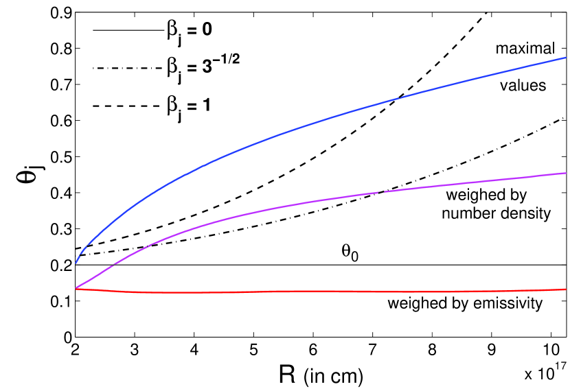
Figure 2.— Evolution of the jet half-opening angle $\theta_{j}$ as a function of radius $R$, for various illustrative cases. The solid line shows the evolution derived from 2D hydrodynamical simulations (Granot et al., 2001). The different lines give the maximal polar angle $\theta$ of the shock front (which is obtained at a relatively small radius where a minor fraction of the emission is produced), and the average values of $\theta$ within the jet when averaged over the circumburst gas density and over the total emissivity. Most of the emission comes from within the original jet opening angle, $\theta_{0}=0.2$. Also shown is the evolution of $\theta_{j}(R)$ predicted by simple semi-analytic models. Three illustrative cases are depicted where the lateral expansion speed is assumed to be $\beta_{j}=0$, $3^{-1/2}$ and $1$ in the local rest frame (Rhoads, 1999; Sari, Piran & Halpern, 1999; Oren, Nakar & Piran, 2004). Since the onset of lateral expansion in the simple models takes place at a somewhat larger radius ($R_{j}$), a higher value of gas density is adopted for these models in order to show more easily their different qualitative behaviors.

In this section we concentrate on a viewing angle along the jet axis, $\theta_{\rm obs}=0$, and in the next section we briefly outline the expected differences for $0<\theta_{\rm obs}<\theta_{0}$. For $\theta_{\rm obs}=0$, the observed image is symmetric around the line-of-sight (to the extent that the jet is axisymmetric). At $t<t_{j}$ the edge of the jet is not visible and the observed image is the same as for a spherical flow: $R_{\perp}\propto(E_{\rm iso}/A)^{1/2(4-k)}t^{(5-k)/2(4-k)}\propto(E/A)^{1/2(3-k)}t_{j}^{-1/2(4-k)}t^{(5-k)/2(4-k)}$ for an external density profile $\rho_{\rm ext}=Ar^{-k}$, i.e. $a=(5-k)/2(4-k)$ where $a\equiv d\ln R_{\perp}/d\ln t$. Here $E$ is the true kinetic energy of the jet, and $E_{\rm iso}=f_{b}^{-1}E$ is the isotropic equivalent energy where $f_{b}=1-\cos\theta_{0}\approx\theta_{0}^{2}/2$ is the beaming factor. At $t<t_{j}$ the flow is described by the Blandford-McKee (1976) self similar solution, which provides an accurate expression for the image size (Granot, Piran & Sari, 1999a; Granot & Sari, 2002),

$$R_{\perp} = \left[\frac{2^{2-k}(17-4k)(4-k)^{5-k}E_{\rm iso}c^{3-k}t^{5-k}}{\pi(5-k)^{5-k}(1+z)^{5-k}A}\right]^{1/2(4-k)}$$

$$= \left\{\begin{matrix}3.91\times 10^{16}(E_{\rm iso,52}/n_{0})^{1/8}[t_{\rm days}/(1+z)]^{5/8}\;{\rm cm}&\ \ (k=0)\cr&\cr 2.39\times 10^{16}(E_{\rm iso,52}/A_{*})^{1/4}[t_{\rm days}/(1+z)]^{3/4}\;{\rm cm}&\ \ (k=2)\end{matrix}\right.\ .$$ (5)

At $t>t_{\rm NR}$ the jet gradually approaches the Sedov-Taylor self similar solution, asymptotically reaching $R_{\perp}\propto(Et^{2}/A)^{1/(5-k)}$, i.e. $a=2/(5-k)$. At $t_{j}<t<t_{\rm NR}$ there is a large uncertainty in the hydrodynamical evolution of the jet, and in particular its rate of sideways expansion. We therefore consider two extreme assumptions which should roughly bracket the different possible evolutions of $R_{\perp}(t)$: (1) relativistic lateral expansion in the comoving frame (Rhoads, 1999; Sari, Piran & Halpern, 1999), for which $\theta_{j}\approx\max(\theta_{0},\gamma^{-1})$ so that at $t_{j}<t<t_{\rm NR}$ we have $\gamma\approx\theta_{j}^{-1}\approx\theta_{0}^{-1}\exp(-R/R_{j})$, and (2) little or no lateral expansion, $\theta_{j}\approx\theta_{0}$ for $t<t_{\rm NR}$, in which case appreciable lateral expansion occurs only when the jet becomes sub-relativistic and gradually approaches spherical symmetry. We shall refer to these models as model 1 and model 2, respectively. Model 2 is also motivated by the results of numerical simulations (see Figure 2) which show only modest lateral expansion as long as the jet is relativistic (Granot et al., 2001; Kumar & Granot, 2003; Cannizzo, Gehrels & Vishniac, 2004). These numerical results are also supported by a simple analytic argument that relies on the shock jump conditions for oblique relativistic shocks (Kumar & Granot, 2003).

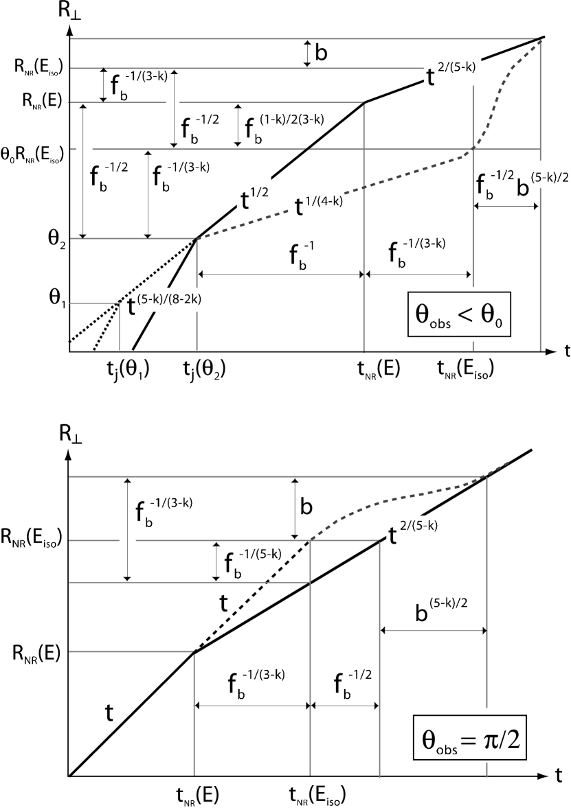
Figure 3.— Schematic plot of the evolution of the observed afterglow image size $R_{\perp}$ of a uniform GRB jet with sharp edges. The jet is either viewed from within the initial jet opening angle, $\theta_{\rm obs}<\theta_{0}$ (upper panel), or from $\theta_{\rm obs}\approx 90^{\circ}$ (lower panel). The solid line is for model 1 (relativistic lateral expansion in the local rest frame) and the dashed line is for model 2 (little or no lateral expansion before $t_{\rm NR}$). The dotted line in the upper panel represents jets (in model 2) with a smaller $\theta_{0}$ and the same true energy $E$, which converge to the same self similar dynamics and therefore the same $R_{\perp}(t)$ after the jet break time $t_{j}$. Also shown are the ratios of various values of $R_{\perp}$ and $t$.

Figure 3 schematically shows the evolution of $R_{\perp}(t)$ for these two extreme models, both when viewed on-axis ($\theta_{\rm obs}<\theta_{0}$) as required for seeing the prompt gamma-ray emission, and for $\theta_{\rm obs}\approx 90^{\circ}$ as will typically be the case for GRB jets found in nearby SNe Type Ib/c (Paczyński, 2001; Granot & Loeb, 2003; Granot & Ramirez-Ruiz, 2004; Ramirez-Ruiz & Madau, 2004). For $\theta_{\rm obs}<\theta_{0}$ at $t_{j}<t<t_{\rm NR}$ we have $R_{\perp}\propto(E/A)^{1/2(3-k)}t^{1/2}$ for model 1, and $R_{\perp}\propto(E_{\rm iso}t/A)^{1/(4-k)}\propto(E/A)^{1/(3-k)}(t/t_{j})^{1/(4-k)}$ for model 2. Therefore, with $k=2$ we have $a=1/2$ for both models, despite their very different jet dynamics. For $k=0$ we have $a=1/2$ for model 1 and $a=1/4$ for model 2.

In model 1, the jet is already relatively close to being spherical (i.e. $\theta_{j}\sim 1$) at $t_{\rm NR}=t_{\rm NR}(E)$, where $R_{\rm NR}(E)=ct_{\rm NR}(E)=[(3-k)E/4\pi Ac^{2}]^{1/(3-k)}$, and its radius is similar to that of the Sedov-Taylor solution , $R_{\rm ST}(E,t)=\xi(Et^{2}/A)^{1/(5-k)}$, corresponding to the same time $t$, where $\xi=\xi(k,\hat{\gamma})\sim 1$. Therefore, we expect it to approach spherical symmetry on a few dynamical times, i.e. when the radius increases by a factor of $b\sim{\rm a\ few}$, corresponding to a factor of $\sim b^{(5-k)/2}$ in time, and the transition between the asymptotic power laws in $R_{\perp}(t)$ is expected to be smooth and monotonic.

In model 2, however, the jet becomes sub-relativistic only at $R_{\rm NR}(E_{\rm iso})=ct_{\rm NR}(E_{\rm iso})$, which is a factor of $\sim(E_{\rm iso}/E)^{1/(3-k)}=f_{b}^{-1/(3-k)}\sim\theta_{0}^{-2/(3-k)}$ larger than $R_{\rm NR}(E)=ct_{\rm NR}(E)$ and a factor of $\sim f_{b}^{-1/(5-k)}\sim\theta_{0}^{-2/(5-k)}$ larger than $R_{\rm ST}[E,t_{\rm NR}(E_{\rm iso})]$. It also keeps its original opening angle, $\theta_{j}\approx\theta_{0}$ until $t_{\rm NR}(E_{\rm iso})$, and hence at this time the jet is still very far from being spherical. Thus, once the jet becomes sub-relativistic, we expect it to expand sideways significantly, and become roughly spherical only when it has increased its radius by a factor of $b\sim{\rm a\ few}$. This should occur, however, roughly at a time $t_{\rm sph}$ when $R_{\rm ST}(E,t_{\rm sph})=bR_{\rm NR}(E_{\rm iso})$, i.e.

$$t_{\rm sph}/t_{\rm NR}(E_{\rm iso})\approx f_{b}^{-1/2}b^{(5-k)/2}\approx\sqrt{2}\,\theta_{0}^{-1}b^{(5-k)/2}\ .$$ (6)

This is a factor of $\sim f_{b}^{-1/2}\approx 14(\theta_{0}/0.1)^{-1}$ larger than the expected transition time in model 1, and for $b\sim 2-3$ gives a factor of $\sim(80-220)(\theta_{0}/0.1)^{-1}$ for $k=0$ and $\sim(40-70)(\theta_{0}/0.1)^{-1}$ for $k=2$. During this transition time, $R_{\perp}(\theta_{\rm obs}<\theta_{0})$ grows by a factor of $\sim f_{b}^{-1/2}b\sim\theta_{0}^{-1}b$ while $R_{\perp}(\theta_{\rm obs}\approx 90^{\circ})$ grows by a factor of $\sim b$. This implies that during the transition,

$$\langle a\rangle=\left\{\begin{matrix}\frac{\ln b-(1/2)\ln f_{b}}{[(5-k)/2]\ln b-(1/2)\ln f_{b}}&(\theta_{\rm obs}<\theta_{0})\cr&\cr\frac{\ln b}{[(5-k)/2]\ln b-(1/2)\ln f_{b}}&(\theta_{\rm obs}=90^{\circ})\end{matrix}\right.\ ,$$ (7)

and $0<\langle a\rangle<2/(5-k)$ for $\theta_{\rm obs}<\theta_{0}$ while $2/(5-k)<\langle a\rangle<1$ for $\theta_{\rm obs}=90^{\circ}$, where $\langle a\rangle\approx 2/(5-k)$ in the limit $b\gg\theta_{0}^{-1}$ (which is not very realistic). The other limiting value of $\langle a\rangle\approx 0$ for $\theta_{\rm obs}<\theta_{0}$ and $\langle a\rangle\approx 1$ for $\theta_{\rm obs}=90^{\circ}$ is approached in the limit $b\ll\theta_{0}^{-1}$. Typical parameter values ($b\sim 2-3$, $\theta_{0}\sim 0.05-0.2$) are somewhat closer to the latter limit. For example, for $k=0$, $b=2.5$ and $\theta_{0}=0.1$ we have $\langle a\rangle\approx 0.722$ for $\theta_{\rm obs}<\theta_{0}$ and $\langle a\rangle\approx 0.185$ for $\theta_{\rm obs}=90^{\circ}$. This demonstrates that for on-axis observers there should be a sharp rise in $R_{\perp}$, while for observers at $\theta_{\rm obs}\approx 90^{\circ}$ there should be a very moderate rise in $R_{\perp}$ during the transition phase from the asymptotic $t_{j}\ll t\ll t_{\rm NR}$ and $t\gg t_{\rm NR}$ regimes. Furthermore, as is illustrated in Figure 3, this transition would not be monotonic in model 2. This is because during the transition $a$ passes through values larger (smaller) than both of its asymptotic values for $\theta_{\rm obs}<\theta_{0}$ ($\theta_{\rm obs}\approx 90^{\circ}$).

For comparison, and in order to perform a quantitative comparison with the data, we consider a simple semi-analytic model where the shock front at any given lab frame time occupies a section of a sphere within $\theta<\theta_{j}$, and $R_{\perp}$ is located at $\theta_{\perp}=\min(\theta_{*},\theta_{j})$. The observer time assigned to a given $\theta_{\perp}(t_{\rm lab})$ is $t=t_{\rm lab}-[R(t_{\rm lab})/c]\cos\theta_{\perp}(t_{\rm lab})$. We follow Oren, Nakar & Piran (2004) with minor differences: (i) we choose the normalization of $R_{\perp}$ at $t\ll t_{j}$ so that it will coincide with the value given by the Blanford-McKee solution (i.e. Eq. 5), and (ii) the lateral spreading verlocity in the comoving frame, $\beta_{j}$, for model 2 smoothly varies from $\beta_{j}\ll 1$ at $t\ll t_{\rm NR}$ to the sound speed, $\beta_{j}\approx c_{s}/c$, at $t>t_{\rm NR}$. The latter is achieved by taking $\beta_{j}$ to be the sound speed suppressed by some power of $\Gamma$.

Figure 4 shows the resulting $R_{\perp}(t)$ for ISM ($k=0$) and stellar wind ($k=2$) environments, and different recipes for $\beta_{j}$. For a given $\beta_{j}$ recipe, $R_{\perp}(t)$ depends on $E/A$ and $\theta_{0}$. The values of these parameters that were used in Figure 4 are indicated in the figure. For $k=2$ the spread in $R_{\perp}(t)$ for the different $\beta_{j}$ recipes is smaller than for $k=0$. This is understandable since the asymptotic values of $a$ are the same for models 1 and 2. There is still a non-negligible spread, however, as the asymptotic value of $a=1/2$ at $t_{j}\ll t\ll t_{\rm NR}$ is not reached. At $t\gg t_{\rm NR}$ all recipes for $\beta_{j}$ approach the same value of $R_{\perp}(t)$, except for $\beta_{j}=0$ for which $R_{\perp}(t)$ is smaller by a factor of $\sin\theta_{0}$. For $\beta_{j}=0$ and $k=0$ there is a pronounced flattening in $R_{\perp}(t)$ at $\sim 1.2\;$day, which is a factor of $\sim 7$ larger than the value of $t_{j}=0.165\;$days that is implied by Eq. (2). We must stress that this simple model becomes unrealistic around $t_{\rm NR}$.

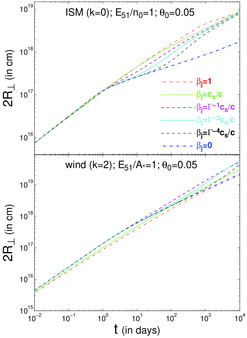
Figure 4.— Evolution of the source size (or more precicely, its diameter $2R_{\perp}$) as a function of time, for a uniform density environment ($k=0$, upper panel) and for a stellar wind ($k=2$, lower panel). Different recipes are considered for the lateral spreading velocity in the comoving frame, $\beta_{j}$. See text for more details.

The apparent velocity of a point source is $\beta_{\rm ap}=\beta\sin\theta/(1-\beta\cos\theta)$. For $\theta_{\rm obs}>\theta_{0}$, as long as $\theta_{j}<\theta_{\rm obs}$ and $t<t_{\rm NR}$ we have $\beta_{\rm ap}\approx 2\Gamma_{\rm sh}^{2}\theta/[1+(\Gamma_{\rm sh}\theta)^{2}]\approx 2/\theta$. For $\theta_{\rm obs}=\pi/2$ we have $\beta_{\rm ap}=\beta_{\rm sh}$ which is close to 1 at $t<t_{\rm NR}$. For $\Gamma_{\rm sh}\gg 1$ and $\theta>\Gamma_{\rm sh}^{-1}$ we have $\beta_{\rm ap}\approx\sin\theta/(1-\cos\theta)$, so that $\beta_{\rm ap}>1$ for $\theta_{\rm obs}<\pi/2$ and $\beta_{\rm ap}<1$ for $\theta_{\rm obs}>\pi/2$ (i.e. for the counter jet, assuming a double sided jet; see Figure 2 of Granot & Loeb, 2003). For $\theta_{\rm obs}<\theta_{0}$ we have $\beta_{\rm ap}=\Gamma_{*}\beta_{*}\approx\Gamma_{*}$ at $t<t_{\rm NR}$. At $t<t_{j}$ we get $\theta_{\perp}=\theta_{*}<\theta_{0}$ and the shock front is roughly spherical with an approximately uniform Lorentz factor within $\theta\lesssim\theta_{*}$, so that $\Gamma_{*}\approx\Gamma_{\rm sh}$. At $t_{j}<t<t_{\rm NR}$ we have $\theta_{*}\approx\theta_{j}\approx\Gamma_{\rm sh}^{-1}$ and $\beta_{\rm ap}\approx\Gamma_{*}\approx\Gamma_{\rm sh}$ for model 1, suggesting that using $\Gamma(\theta_{*})$ for calculating the emission (i.e. in Eqs. 1, 3 and 8) is a reasonable approximation. For model 2, $\theta_{*}\approx\theta_{j}\approx\theta_{0}$ and $\beta_{\rm ap}\approx\Gamma_{*}\approx 2\theta_{0}\Gamma_{\rm sh}^{2}$, so that $\Gamma_{*}/\Gamma_{\rm sh}\approx 2\theta_{0}\Gamma_{\rm sh}<1$ suggesting that $\Gamma(\theta_{*})$ underestimates the effective value of the emissivity-weighted $\Gamma$ , which enters the expressions for the observed emission. This results from the fact that in model 2 most of the emission at $t_{j}<t<t_{\rm NR}$ originates from $\theta<\theta_{0}$ where $\Gamma$ is higher than at $\theta_{*}\gtrsim\theta_{0}$ (see Figure 2 and Granot et al., 2001).

4. Linear Polarization

For $0<\theta_{\rm obs}<\theta_{0}$ the image would not be symmetric around the line-of-sight, but its typical angular size would be similar to that of $\theta_{\rm obs}=0$. If there is significant lateral spreading at $t>t_{j}$, then this should cause the image to become more symmetric around our line-of-sight with time. This, by itself, might be a possible diagnostic for the degree of lateral spreading. The degree of asymmetry in the observed image should also be reflected in the degree of linear polarization, and its temporal evolution. While the image might be resolved only for a very small number of sufficiently nearby GRBs, the linear polarization might be measured for a larger fraction of GRBs.

Contrary to naive expectations, for very slow lateral expansion ($\beta_{j}\ll 1$) the polarization decays faster after its peak at $t\sim t_{j}$ compared to lateral expansion at the local sound speed, $\beta_{j}=c_{s}/c\approx 3^{-1/2}$, in the comoving frame (Rossi et al., 2004). A very fast lateral expansion in the local frame close to the speed of light ($\beta_{j}\approx 1$), leads to $\theta_{j}\approx\max(\theta_{0},\gamma^{-1})$ and to three peaks in the polarization light curve, where the polarization position angle changes by $90^{\circ}$ as the degree of polarization passes through zero between the peaks (Sari, 1999). When there is a slower lateral expansion or no lateral expansion at all (Ghisellini & Lazzati, 1999), there are only two peaks in the polarization lightcurve where again the polarization position angle changes by $90^{\circ}$ as the degree of polarization passes through zero between the peaks. The peak polarization is higher for $\beta_{j}\approx 0$ ($\sim 15\%-16\%$) compared to $\beta_{j}=3^{-1/2}$ ($\sim 9\%$) (Rossi et al., 2004). The maximal observed degree of polarization is, however, usually $\lesssim 3\%$ suggesting that the magnetic field configuration behind the shock is more isotropic than a random field fully within the plane of the shock (Granot & Königl, 2003) which is expected if the magnetic field is produced by the Weibel instability (Medvedev & Loeb, 1999). This changes the overall normalization of the polarization light curve, and hardly affects its shape (Granot & Königl, 2003). Since the overall normalization is the most pronounced difference between slow and fast lateral expansion, and it is very similar to the effect of the degree of anisotropy of the magnetic field behind the shock, it would be very hard to constrain the degree of lateral expansion from the polarization light curves. There are also other possible complications, such as a small ordered magnetic field component (Granot & Königl, 2003) which can induce polarization that is not related to the jet structure.

Taylor et al. (2004) put a $3\;\sigma$ upper limit of $1\%$ on the linear polarization in the radio ($\nu=8.4\;$GHz) at $t=7.71\;$days. They attribute the low polarization to synchrotron self absorption. Indeed, $\nu_{sa}$ is above $8.4\;$GHz at this time, but only by a factor of $\sim 2$. One might expect a suppression of the polarization in the self absorbed region of the synchrotron spectrum since it should follow the Rayleigh-Jeans part of a black body spectrum, and depend only on the electron distribution (i.e. the “effective temperature”) and not on the details of the magnetic field (Granot, Piran & Sari, 1999b). The optical depth to self absorption does, however, depend on the details of the magnetic field, and may thereby vary with the direction of polarization. Therefore, there might still be polarization at $\nu\lesssim\nu_{sa}$ which will go to zero in the limit $\nu\ll\nu_{sa}$. An ordered magnetic field in the shocked fluid through which the emitted synchrotron radiation propagates on its way to the observer, might induce some polarization in the observed radiation (Sagiv, Waxman & Loeb, 2004). These effects are suppressed roughly by a factor of the square root of the ratio between the magnetic field coherence length and the width of the emitting region (which is of the order of the typical path length of an emitted photon through the shocked plasma before it escapes the system).

5. The Surface Brightness Profile

Taylor et al. (2004) use a circular Gaussian profile for their quoted values, and also tried a uniform disk and thin ring. They find that a Gaussian with an angular diameter size of $1\;$mas is equivalent to a uniform disk with an angular diameter of $1.6\;$mas and a thin ring with an angular diameter of $1.1\;$mas. At $t<t_{j}$ the jet dynamics are close to that of a spherical flow, since the center of the jet is not in causal contact with its edge, and the dynamics can be described by the Blandford-Mckee (1976) spherical self similar solution (within the jet, at $\theta<\theta_{0}$). The surface brightness in this case has been investigated at length in several works (Waxman, 1997; Sari, 1998; Panaitescu & Mészáros, 1998; Granot, Piran & Sari, 1999a, b; Granot & Loeb, 2001). The surface brightness profile of the image, normalized by its average value across the image, is the same within each power law segment of the spectrum, but changes between different power law segments (Granot & Loeb, 2001). The afterglow image is limb brightened, resembling a ring, in the optically thin part of the spectrum and more uniform, resembling a disk, at the self absorbed part of the spectrum. This can affect the angular size of the image that is inferred from the observations (Taylor et al., 2004), where the angular diameter for a uniform disk (thin ring) is a factor of 1.6 (1.1) larger than the values quoted by Taylor et al. (2004) for a circular Gaussian surface brightness profile. This effect would be more important at $\nu\lesssim\nu_{sa}$ where the afterglow image resembles a uniform disk rather than a thin ring.

One should keep in mind that the image size of GRB 030329 was inferred well after the jet break time, $t\gg t_{j}$, and relatively close to the non-relativistic transition time, $t\sim t_{\rm NR}$. However, at $t_{j}<t<t_{\rm NR}$ the jet dynamics is poorly known, and this uncertainty must necessarily be reflected in any calculation of the afterglow image at this stage, which could only be as good as the assumed dynamical model for the jet. The afterglow image at this stage was calculated by Ioka & Nakamura (2001) assuming lateral expansion at the local sound speed (Rhoads, 1999), similar to our model 1. They find that at $t<t_{j}$ the surface brightness diverges at the outer edge of the image, which is an artifact of their assumption of emission from a two dimensional surface (Sari, 1998; Granot & Loeb, 2001) identified with the shock front. Calculating the contribution from all the volume of the emitting fluid behind the shock makes this divergence go away, except for certain power law segments of the spectrum where the emission indeed arises from a very thin layer just behind the shock (Granot & Loeb, 2001). At $t>t_{j}$ Ioka & Nakamura (2001) obtain a relatively uniform surface brightness profile. However, this is due to the unphysical assumption that the shock front at any given lab frame time is part of a sphere within some finite angle $\theta_{j}$ from the jet symmetry axis where the jet ends abruptly. The edge of the image in this case corresponds to this un-physical point where the jet ends abruptly (see Figure 5). More physically, as is shown by numerical simulations (Granot et al., 2001), the shock front is not a section of a sphere and is instead round without any sharp edges. Similarly to the spherical-like evolution at $t<t_{j}$, the edge of the image would in this case correspond to $R_{\perp}=\max(R\sin\theta)$, and thus the image is expected to be limb brightened for the same qualitative reasons that apply at $t<t_{j}$, even though there would be some quantitative differences. A proper calculation of the afterglow image at $t>t_{j}$ requires full numerical simulations of the jet dynamics.

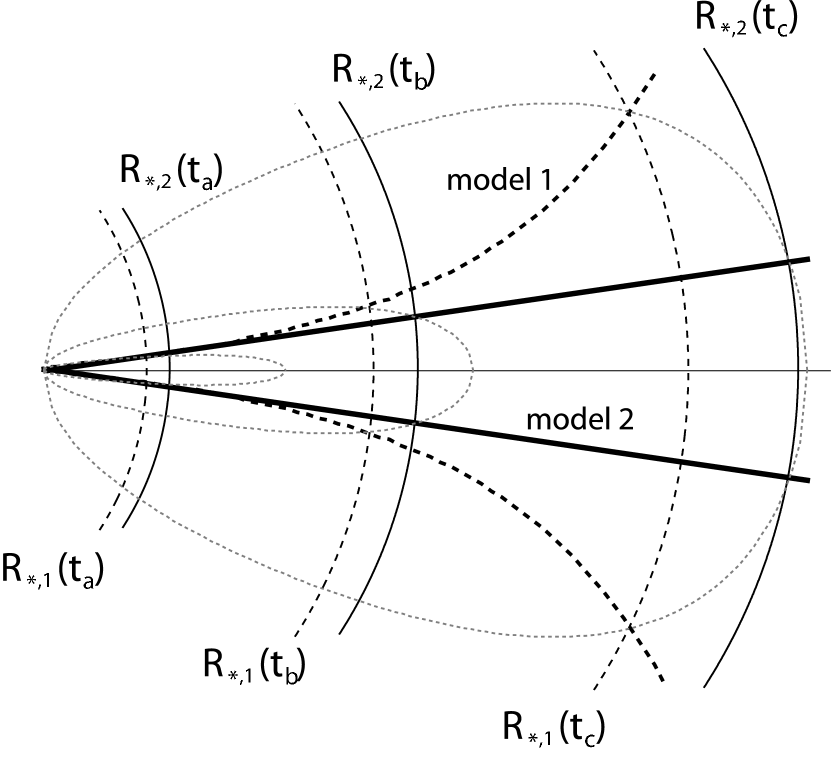
Figure 5.— Evolution of the source size as a function of time for $t>t_{j}$. In model 1, the lateral expansion in the local frame is relativistic while in model 2 there is no lateral expansion at $t>t_{j}$. The shock front at any given time $t_{\rm lab}$ is assumed to be part of a sphere which abruptly ends at a finite angle $\theta_{j}$ from the jet axis. The gray dotted lines represent the equal arrival time surfaces at three different observed times. Since the jet dynamics, $R(t_{\rm lab})$, are different for models 1 and 2, the equal arrival time surfaces should be different (but in this sketch, for simplicity, we depicted them as being equal). At $t>t_{j}$ (where $\theta_{j}(R_{*})<\theta_{*}$), the edge of the image which determines the image size is located at the edge of the jet, i.e. at an angle $\theta_{j}$ instead of $\theta_{*}$.

6. Application to GRB 030329

We now apply the expressions derived in the previous section to GRB 030329 which occurred at a redshift of $z=0.1685$. We use the image angular diameter size of $\theta_{s}\approx 70\;{\rm\mu}$as for $D_{A}\approx 587\;$Mpc that was inferred at $t=24.5\;$days (Taylor et al., 2004), which corresponds to $R_{\perp}\approx 0.1\;$pc. This implies an average apparent speed of $\langle\beta_{\rm ap}\rangle=(1+z)R_{\perp}/ct\approx 5.66$. The instantaneous apparent speed is given by $\beta_{\rm ap}\equiv[(1+z)/c]dR_{\perp}/dt=a\langle\beta_{\rm ap}\rangle$ where $a\equiv d\ln R_{\perp}/d\ln t$. For GRB 030329, if we also take into account the inferred source size of $\theta_{s}\approx 170\;{\rm\mu}$as or $R_{\perp}\approx 0.25\;$pc at $t=83.3\;$days and the $2\;\sigma$ upper limit of $\theta_{s}<100\;{\rm\mu}$as or $R_{\perp}<0.14\;$pc at $t=51.3\;$days (Taylor et al., 2004), we have $a=0.71_{-0.3}^{+0.4}$ ($1\;\sigma$). This value is between $t=24.5\;$days and $83.3\;$days, assuming that $R_{\perp}(t)$ followed a perfect power law behavior $\propto t^{a}$ with $a={\rm const}$ during this time. This is a reasonable approximation for model 1 or model 2 with $k=2$ for which $a=1/2$ at $t_{j}<t<t_{\rm NR}$ and therefore these models are consistent with the observed temporal evolution of the image size. For model 1 with $k=0$ (see §3) $a=1/4$ at $t_{j}\ll t\ll t_{\rm NR}$ but its value is expected to increase significantly near $t_{\rm NR}$ which we find to be at $\sim 200\;$days for this model (see Table 1). Therefore, it can still account for the observed image size at $t=24.5\;$days and $83.3\;$days together with the upper limits at $51.3\;$days. At $t=24.5\;$days, however, we still expect the value of $a$ in model 2 with $k=0$ to be relatively close to its asymptotic value of $a=1/4$.

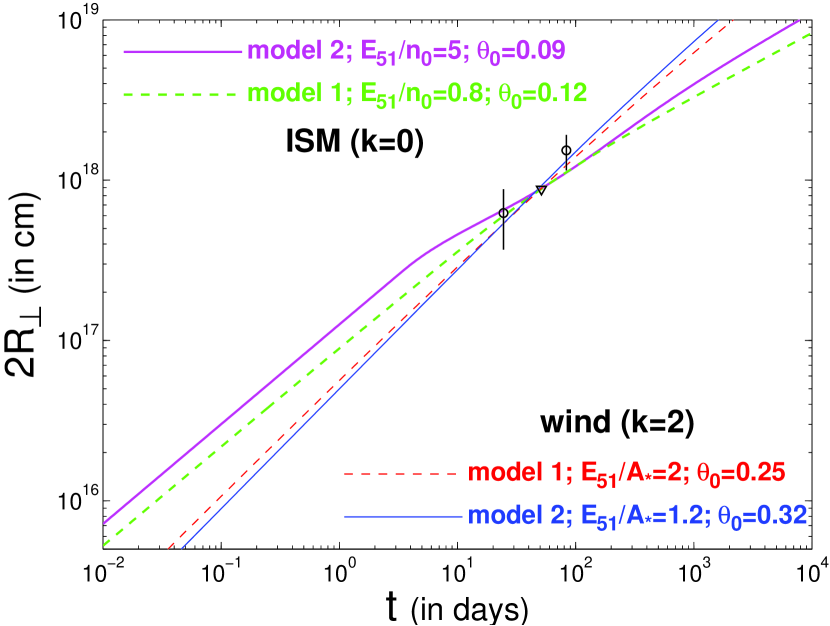
Figure 6.— A tentative fit of a simple semi-analytic realization of models 1 and 2 to the observed image size (of diameter $2R_{\perp}$). The physical parameters and external density profile for each model are indicated.

Figure 6 shows crude fits between the simple semi-analytic realization of models 1 and 2 (that is described at the end of §3) and the observed image size (Taylor et al., 2004). For model 2 we have used the recipe $\theta_{j}=\Gamma^{-1}(c_{s}/c)$ for the lateral expansion. We have treated the value of $E/A$ as a free parameter whose value was varied in order to get a good fit, while the value of $\theta_{0}$ was determined according to the observed jet break time $t_{j}\approx 0.5\;$days using Eq. (2). In the latter procedure we take into account an increase in energy by a factor of $f\sim 10$ due to refreshed shocks (Granot, Nakar & Piran, 2003) between $t_{j}$ and the times when the image size was measured. For simplicity, we do not include the effect of the energy injection on the early image size. The image size that is calculated in this way to not valid before the end of the energy injection episode (after several days), but it should be reasonably accurate at $t\gtrsim 25\;$days when its value had been measured. The values of $E/A$ and $\Gamma(25\;d)$ from these fits are indicated in Figure 6 and in Table 1.

For $a=(0.25,0.5,0.75)$ we obtain $\beta_{\rm ap}\approx(1.4,2.8,4.2)$, $\Gamma_{*}\approx(1.7,3.0,4.4)$ and $\Gamma(\theta_{*})\approx(1.5,2.4,3.4)$. The values of $\Gamma(\theta_{*})$ are similar to the value of $\Gamma$ that were obtained from the fit to the observed image size for model 1 and model 2 with $k=2$, but it is smaller for model 1 with $k=0$, as expected (see discussion at end of §3).

Using the radio data from Berger et al. (2003), we find that $F_{\nu}\approx 10\;$mJy at $t\approx 25\;$days and $\nu=4.86\;$GHz which according to the spectrum at this time is below $\nu_{sa}$. Berger et al. (2003) also estimated the break frequencies at $t\approx 10\;$days to be $\nu_{sa}\approx 19\;$GHz and $\nu_{m}\approx 43\;$GHz, which is consistent with $\nu<\nu_{sa}<\nu_{m}$ at $t=24.5\;$days. A value of $p=2.25$ was inferred for GRB 030329 (Willingale et al., 2004). For the power law segment of the spectrum where $F_{\nu}\propto\nu^{2}$ (labeled ‘B’ in Figure 1 of Granot & Sari, 2002) we have $\gamma_{\rm eff}\approx\gamma_{m}$ for which Eqs. (1) and (3) imply

$$\epsilon_{e}\approx\frac{1}{2\pi}\left(\frac{p-1}{p-2}\right)\frac{(1+z)}{\Gamma(\Gamma-1)}\left(\frac{D_{A}}{R_{\perp}}\right)^{2}\frac{F_{\nu}}{m_{p}\nu^{2}}\ .$$ (8)

Using the above values for the flux, $R_{\perp}$, $\Gamma(\theta_{*})$ and $p$ for GRB 030329, Eq. (8) gives $\epsilon_{e}\approx(0.10,0.023,0.0099)$ for $a=(0.25,0.5,0.75)$. These values of $\epsilon_{e}$ are somewhat on the low side compared to the values inferred from broad band afterglow modelling of other afterglows (e.g., Panaitescu & Kumar, 2001b). In Table 1 we show in addition to these values of $\epsilon_{e}$, also the values that are obtained when evaluating $\Gamma$ from the fit to the image size that is shown in Figure 6. The largest difference between these two estimates of $\epsilon_{e}$ is for model 1 with $k=0$, for which evaluating $\Gamma$ from the fit to the observed source size probably provides a more accurate estimate.

Since Eq. (8) relies on a small number of assumptions, it is rather robust. However, the value of $\epsilon_{e}$ in equation (8) is very sensitive to the value of $R_{\perp}$. This is because $\epsilon_{e}\propto 1/R_{\perp}^{2}\Gamma(\Gamma-1)$ and for $\Gamma\gg 1$ we have $\Gamma\approx\Gamma_{*}/\sqrt{2}\approx\beta_{\rm ap}/\sqrt{2}=a\langle\beta_{\rm ap}\rangle/\sqrt{2}\propto R_{\perp}$ so that $\epsilon_{e}\propto R_{\perp}^{-4}$. For example, $\theta_{s}=45\;\mu$as ($R_{\perp}=0.064\;$pc) at $t=24.5\;$days, which is still within the measurement errors, would imply $\epsilon_{e}=(0.61,0.14,0.060)$ for $a=(0.25,0.5,0.75)$. The latter values, especially for $a\approx 0.5$, are consistent with the value found by Willingale et al. (2004) from a broad band fit to the afterglow data: $\epsilon_{e}=0.24$ and $0.18<\epsilon_{e}<0.31$ at the $90\%$ confidence level, and with the value of $\epsilon_{e}\approx 0.16$ found by Berger et al. (2003).

7. Inferring the Physical Parameters from a Snapshot Spectrum at $t_{j}<t<t_{\rm NR}$

For model 1, we obtain expressions for the peak flux and break frequencies at $t_{j}<t<t_{\rm NR}$ by using the expressions for $t<t_{j}$ from Granot & Sari (2002) in order to estimate their values at $t_{j}$, and then using the their temporal scalings at $t_{j}<t<t_{\rm NR}$ from Rhoads (1999) and Sari, Piran & Halpern (1999). In Appendix C we provide expressions for the peak flux and break frequencies as a function of the physical parameters and solve them for the physical parameter as a function of the peak flux and break frequencies for both models 1 and 2. The results for GRB 030329 are given below.

For GRB 030329, Berger et al. (2003) infer $\nu_{sa}\approx 19\;$GHz, $\nu_{m}\approx 43\;$GHz and $F_{\nu,{\rm max}}\approx 96\;$mJy at $t\approx 10\;$days, as well as $p=2.2$. Using Eqs. 4.13-4.16 of Sari & Esin (2001), Berger et al. (2003) find $E_{\rm iso,52}\approx 0.56\nu_{c,13}^{1/4}$, $n_{0}\approx 1.8\nu_{c,13}^{3/4}$ $\epsilon_{B}\approx 0.10\nu_{c,13}^{-5/4}$, $\epsilon_{e}\approx 0.16\nu_{c,13}^{1/4}$, and using a value of $\theta_{j}\approx 0.3$ at this time they inferred $E_{51}\approx 0.25$. For the same values of the spectral parameters and using our model 1 we obtain $E_{\rm iso,52}=0.16\nu_{c,13}^{1/4}$, $E_{51}=0.36\nu_{c,13}^{3/8}$, $n_{0}=15\nu_{c,13}^{3/4}$, $\epsilon_{B}=0.12\nu_{c,13}^{-5/4}$, $\epsilon_{e}=0.24\nu_{c,13}^{1/4}$ for $k=0$ and $E_{\rm iso,52}=0.10\nu_{c,13}^{1/4}$, $E_{51}=0.43\nu_{c,13}^{3/8}$, $A_{*}=1.4\nu_{c,13}^{1/2}$, $\epsilon_{B}=0.034\nu_{c,13}^{-5/4}$, $\epsilon_{e}=0.36\nu_{c,13}^{1/4}$ for $k=2$. The implied values of $E/A$ are shown in Table 1. The differences between our values and those of Berger et al. (2003) arise from differences by factors of order unity between the coefficients in the expressions for the peak flux and break frequencies. This typically results in differences by factors of order unity in the inferred values of the physical parameters. The difference in the external density $n$ is relatively large since it contains high powers of $\nu_{sa}$ and $\nu_{m}$ (Granot, Piran & Sari, 1999b) making it more sensitive to the exact theoretical expressions and observational values of these frequencies.

For model 1 and $k=0$ we obtain $E_{51}/n_{0}=0.0.024\nu_{c,13}^{-3/8}$ compared to $E_{51}/n_{0}=0.14\nu_{c,13}^{-1/2}$ of Berger et al. (2003) and $E_{51}/n_{0}\sim 0.8$ that we obtain from the fit to the observed image size (Figure 6). Because of the large uncertainty in the value of $n$ that is determined from the snapshot spectrum, and the large uncertainty in the value of $E/n$ from the fit to the image size, these values are consistent with each other within their reasonable errors (see Table 1). For model 1 and $k=2$ we obtain $E_{51}/A_{*}=0.31\nu_{c,13}^{-1/8}$ compared to $E_{51}/A_{*}\approx 0.8$ from the fit to the observed image size. Here the difference between the two values is smaller, but the uncertainty on the two values is also smaller (see Table 1). Altogether, the two values are still consistent within their estimated errors.

For our model 2 involving a jet with no significant lateral spreading, the peak flux is suppressed by a factor of $(t/t_{j})^{-(3-k)/(4-k)}$ where $t_{j}\approx 0.5\;$days and $t/t_{j}\approx 20$, i.e. a factor of $\approx 0.11$ for $k=0$ and $\approx 0.22$ for $k=2$. This implies (see appendix C) $E_{\rm iso,52}=4.7\nu_{c,13}^{1/4}$, $E_{51}=0.21\nu_{c,13}^{3/8}$, $n_{0}=0.53\nu_{c,13}^{3/4}$, $\epsilon_{B}=0.37\nu_{c,13}^{-5/4}$, $\epsilon_{e}=0.078\nu_{c,13}^{1/4}$ for $k=0$ and $E_{\rm iso,52}=0.98\nu_{c,13}^{1/4}$, $E_{51}=0.29\nu_{c,13}^{3/8}$, $A_{*}=1.4\nu_{c,13}^{1/2}$, $\epsilon_{B}=0.071\nu_{c,13}^{-5/4}$, $\epsilon_{e}=0.17\nu_{c,13}^{1/4}$ for $k=2$. For model 2 with $k=0$ we get $E_{51}/n_{0}=0.40\nu_{c,13}^{-3/8}$ compared to $E_{51}/n_{0}\approx 5$ from the fit to the observed image size. These two values are consistent within the large uncertainties on both values (see Table 1).

For model 2 with $k=2$ we obtain $E_{51}/A_{*}=0.10\nu_{c,13}^{-1/8}$ compared to $E_{51}/A_{*}\approx 1.2$ from the fit to the observed image size. In this case, however, the errors on these two values are relatively small (see Table 1). This is because: (i) the image size is linear in $E/A$ which corresponds to a relatively strong dependence, and therefore the observed image size can constrain the value of $E/A$ relatively well, and (ii) the expression for $E/A$ from the spectrum contains relatively small powers of the break frequencies and peak flux and thus has a correspondingly small uncertainty. Therefore, the two values of $E_{51}/A_{*}$ are farther apart than is expected from the uncertainty on these values. Thus, one might say that the data disfavors model 2 with $k=2$. It is hard, however, to rule out this model altogether, because of the uncertainty is the exact expressions for the break frequencies and peak flux at $t_{j}<t<t_{\rm NR}$.

8. Discussion

We have analyzed the data on the time-dependent image size of the radio afterglow of GRB 030329 (Taylor et al. 2004) and constrained the physical parameters of this explosion. The image size was measured after the jet break time $t_{j}$ in the afterglow lightcurve, where existing theoretical models still have a high level of uncertainty regarding the jet dynamics. This motivated us to consider two extreme models for the lateral expansion of the jet: model 1, where there is relativistic lateral expansion in the local rest frame of the jet at $t_{j}<t<t_{\rm NR}$, and model 2, with no significant lateral expansion until the transition time to a non-relativistic expansion $t_{\rm NR}$. We have tested the predictions of these models against the observations, for both a uniform ($\rho_{\rm ext}=Ar^{-k}$, with $k=0$) and a stellar wind ($k=2$) external density profile.

The observational constraints included comparisons between: (i) the value of the post-shock energy fraction in relativistic electrons $\epsilon_{e}$ that is inferred from the source size and flux below the self absorption frequency and its value from the ‘snapshot’ spectrum at $t\approx 10\;$days; (ii) the value of $E/A$ that is inferred from the source size and its value from the ‘snapshot’ spectrum at $t\approx 10\;$days; and (iii) the observed temporal evolution of the source size and the theoretical predictions. We have found that most models pass all these tests. The only exception is model 2 with $k=2$, involving a relativistic jet with little lateral expansion (well before $t_{\rm NR}$) that is propagating in a stellar wind external medium, which does poorly on point (ii) above.

We have found that for a jet with little lateral expansion before $t_{\rm NR}$ (our model 2), the jet would become roughly spherical only long after $t_{\rm NR}$ (see Eq. 6 and the discussion around it). This introduces a fast growth in the image size near $t_{\rm NR}$ for on-axis observers with $\theta_{\rm obs}<\theta_{0}$ (see upper panel of Figure 3) that detect the prompt gamma-ray emission (as in the case of GRB 030329). For an observer at $\theta_{\rm obs}\approx 90^{\circ}$ as would typically be the case for GRBs that might be found in nearby SNe Ib/c, months to years after the SN (Paczyński, 2001; Granot & Loeb, 2003; Ramirez-Ruiz & Madau, 2004), this causes a very slow increase in the image size near $t_{\rm NR}$ (see lower panel of Figure 3).

Oren, Nakar & Piran (2004) have considered a jet with no lateral spreading, even at $t\gtrsim t_{\rm NR}$, and concluded that it can be ruled out for a uniform external density ($k=0$) since it gives $a=1/4$ at $t_{j}<t<t_{\rm NR}$ which is inconsistent with observations [recall that in §6 we have found that $a=0.71_{-0.3}^{+0.4}$ ($1\;\sigma$) between 25 and $83\;$days]. In our analysis we have argued that physically one expects lateral spreading to start around $t_{\rm NR}$, even if it is negligible at $t\ll t_{\rm NR}$. We have shown that with this more realistic assumption for the jet dynamics (our model 2) the temporal evolution of the image size for a uniform external density ($k=0$) is consistent with observations.

The formalism developed in this paper would be useful for the analysis of future radio imaging of nearby GRB afterglows. The forthcoming Swift satellite (http://swift.gsfc.nasa.gov/) is likely to discover new GRBs at low redshifts. Follow-up imaging of their radio jets will constrain their physical properties and reveal whether the conclusions we derived for GRB 030329 apply more generally to other relativistic explosions.

Table 1Comparing the values of Physical Parameters derived from different Observables

external	physical	observables			major source	uncertain by
density	parameter	being used	model 1	model 2	of uncertainty	a factor of
		$F_{\nu}(10\,{\rm d})$	$0.024\nu_{c,13}^{-3/8}$	$0.40\nu_{c,13}^{-3/8}$	$\propto\nu_{sa}^{-15/4}\nu_{m}^{-15/8}F_{\nu,{\rm max}}^{9/4}$	$\sim 10-100$
$k=0$	$E_{51}/n_{0}$	$R_{\perp}(t)$	0.8	5	$\propto R_{\perp}^{6\;(3)}$ in model $1\;(2)$	$\sim 10$ ($\sim 5$)
		$F_{\nu}(10\,{\rm d})$	$0.31\nu_{c,13}^{-1/8}$	$0.10\nu_{c,13}^{-1/8}$	$\propto\nu_{sa}^{-5/4}\nu_{m}^{-5/8}F_{\nu,{\rm max}}^{3/4}$	$\sim 2-3$
$k=2$	$E_{51}/A_{*}$	$R_{\perp}(t)$	2	1.2	$\propto R_{\perp}^{3\;(1)}$ in model $1\;(2)$	$\sim 5$ ($\sim 2$)
			2.4	1.5	$R_{\perp}({\rm obs})$ & $\Gamma(\theta_{*})$	$\sim 1.3$
$k=0$	$\Gamma(25\;{\rm d})$	$R_{\perp}$	2.1	2.4	$R_{\perp}({\rm obs})$ & jet model	$\sim 1.1-1.2$
			2.4	2.4	$R_{\perp}({\rm obs})$ & $\Gamma(\theta_{*})$	$\sim 1.3$
$k=2$	$\Gamma(25\;{\rm d})$	$R_{\perp}$	2.6	2.8	$R_{\perp}({\rm obs})$ & jet model	$\sim 1.1-1.2$
			0.023	0.10	$R_{\perp}$ & $\Gamma(\theta_{*})$ in Eq. 8	$\sim 10$
$k=0$	$\epsilon_{e}$	$R_{\perp}$, $F_{\nu<\nu_{sa}}$	0.035	0.024	$R_{\perp}$ & $\Gamma({\rm Fig.\;\ref{R_perp_fit}})$ in Eq. 8	$\sim 5-10$
		$F_{\nu}(10\;{\rm d})$	$0.24\nu_{c,13}^{1/4}$	$0.078\nu_{c,13}^{1/4}$	model & value of $\nu_{c}$	$\sim 3$
			0.023	0.023	$R_{\perp}$ & $\Gamma(\theta_{*})$ in Eq. 8	$\sim 10$
$k=2$	$\epsilon_{e}$	$R_{\perp}$, $F_{\nu<\nu_{sa}}$	0.020	0.017	$R_{\perp}$ & $\Gamma({\rm Fig.\;\ref{R_perp_fit}})$ in Eq. 8	$\sim 5-10$
		$F_{\nu}(10\;{\rm d})$	$0.36\nu_{c,13}^{1/4}$	$0.17\nu_{c,13}^{1/4}$	model & value of $\nu_{c}$	$\sim 3$

Note. — Estimates for the physical parameters of GRB 030329 derived from different observable quantities for different models of the jet lateral expansion. The value of $E/A$ is estimated from the spectrum at $10\;$days (upper line) and from the fit to the observed image size (lower line). The value of $\Gamma(25\;{\rm d})$ is evaluated both as $\Gamma(\theta_{*})$ according to §2 (upper line) and from the fit to the observed image size (lower line). The value of $\epsilon_{e}$ in first two lines is evaluated first using Eq. 8 with the values of $\Gamma(25\;{\rm d})$ from the corresponding lines. In the third line the value of $\epsilon_{e}$ is from the spectrum at $10\;$days (third line).

Appendix A The Angle $\theta_{*}$ on the Equal Arrival Time Surface where $R_{\perp}$ is Located

The time at which a photon emitted at a lab frame time $t_{\rm lab}$ and at spherical coordinates $(r,\theta,\phi)$ reaches the observer is given by

$$t=t_{\rm lab}-(R/c)\cos\theta$$ (A1)

and shall be referred to as the observed time, where for convenience the direction to the observer was chosen to be along the $z$-axis (i.e. at $\theta=0$). Let the location of a spherically symmetric shock front (or any other emitting surface for that matter) be described by $r=R(t_{\rm lab})$ and that of an axially symmetric shock front by $r=R(t_{\rm lab},\theta)$. We shall now calculate the angle $\theta_{*}$ on the equal arrival time surface (which is defined by $t={\rm const}$) where $R_{\perp}=\max(R\sin\theta)$ is located. At this point on the equal arrival time surface we have

$$0=\left(\frac{\partial R\sin\theta}{\partial\theta}\right)_{t}=\left(\frac{\partial R\sin\theta}{\partial\theta}\right)_{t_{\rm lab}}+\left(\frac{\partial R\sin\theta}{\partial t_{\rm lab}}\right)_{\theta}\left(\frac{\partial t_{\rm lab}}{\partial\theta}\right)_{t}=R(\cos\theta+\tilde{R}_{\theta}\sin\theta)+\beta_{r}c\sin\theta\left(\frac{\partial t_{\rm lab}}{\partial\theta}\right)_{t}\ ,$$ (A2)

where we use the notions $(\partial R/\partial t_{\rm lab})_{\theta}=\beta_{r}c$ and $\tilde{R}_{\theta}=(\partial\ln R/\partial\theta)_{t_{\rm lab}}$. From Eq. (A1) we have

$$0=\left(\frac{\partial t}{\partial\theta}\right)_{t}=\frac{R}{c}(\sin\theta-\tilde{R}_{\theta}\cos\theta)+(1-\beta_{r}\cos\theta)\left(\frac{\partial t_{\rm lab}}{\partial\theta}\right)_{t}\ ,$$ (A3)

so that

$$\left(\frac{\partial t_{\rm lab}}{\partial\theta}\right)_{t}=\frac{R}{c}\left(\frac{\tilde{R}_{\theta}\cos\theta-\sin\theta}{1-\beta_{r}\cos\theta}\right)\ .$$ (A4)

Substituting Eq. (A4) into Eq. (A2) we obtain

$$\cos\theta=\beta_{r}-\tilde{R}_{\theta}\sin\theta=\frac{1}{c}\left(\frac{\partial R}{\partial t_{\rm lab}}\right)_{\theta}-\frac{\sin\theta}{R}\left(\frac{\partial R}{\partial\theta}\right)_{t_{\rm lab}}\ .$$ (A5)

For a spherically symmetric shock $\tilde{R}_{\theta}=0$ and $\cos\theta_{*}=\beta_{r}(\theta_{*})=\beta_{*}$, where in this case $\beta_{r}$ is the shock velocity at the point on the equal arrival time surface were $\theta=\theta_{*}$ and $R_{\perp}$ is located. For a shock with axial symmetry we have

$$\cos\theta_{*}=\frac{\beta_{r}-\tilde{R}_{\theta}\sqrt{1-\beta_{r}^{2}+\tilde{R}_{\theta}^{2}}}{1+\tilde{R}_{\theta}^{2}}\ ,$$ (A6)

and

$$\beta_{r}=\beta_{*}\sqrt{1+\tilde{R}_{\theta}^{2}}\ ,$$ (A7)

where $\beta_{*}$ is the shock velocity component normal to the shock front in the rest frame of the upstream medium, which is the one that enters into the shock jump conditions (Kumar & Granot, 2003).

Appendix B The Apparent Velocity

The apparent velocity, $\beta_{\rm ap}=[(1+z)/c](dR_{\perp}/dt)$, for a point source moving with a velocity $\beta$ at an angle $\theta$ from our line-of-sight is

$$\beta_{\rm ap}=\frac{\beta\sin\theta}{1-\beta\cos\theta}\ .$$ (B1)

For a spherical shock front moving at a constant velocity $\beta_{\rm sh}$, $R_{\perp}$ is located at a constant angle $\theta_{*}$ which satisfies $\cos\theta_{*}=\beta_{*}=\beta_{\rm sh}={\rm const}$ (according to Eq. A5) so that the apparent velocity of the edge of the observed image is simply given by substituting $\cos\theta_{*}=\beta_{*}$ in Eq. (B1). This gives

$$\beta_{\rm ap}=\Gamma_{*}\beta_{*}=\sqrt{\Gamma_{*}^{2}-1}\ .$$ (B2)

We shall now show that this result holds for any spherically symmetric shock front. At $t+dt$ we have

$$\theta_{*}(t+dt)=\theta_{*}(t)+d\theta_{*}\quad\quad,\quad\quad\beta_{*}(t+dt)=\beta_{*}(t)+d\beta_{*}\quad\quad,\quad\quad d\beta_{*}=d\cos\theta_{*}\propto dt\ ,$$ (B3)

and since Eq. (B2) holds for a sphere moving at a constant velocity, we have

$$\left[R\sin\theta\right](t+dt,\theta_{*})=R_{\perp}(t)+\Gamma_{*}(t)\beta_{*}(t)cdt+{\mathcal{O}}(dt^{2})\ .$$ (B4)

Now, since $R_{\perp}$ is located where $(\partial R\sin\theta/\partial\theta)_{t}=0$ then

$$R_{\perp}(t+dt)=\left[R\sin\theta\right](t+dt,\theta_{*}+d\theta_{*})=\left[R\sin\theta\right](t+dt,\theta_{*})+{\mathcal{O}}(dt^{2})=R_{\perp}(t)+\Gamma_{*}(t)\beta_{*}(t)cdt+{\mathcal{O}}(dt^{2})\ ,$$ (B5)

and therefore Eq. (B2) holds for any spherically symmetric shock front.

Finally, for an axially symmetric shock front, we obtain based on similar considerations as in the spherical case

$$\beta_{\rm ap}=\frac{\beta_{r}\sin\theta_{*}}{1-\beta_{r}\cos\theta_{*}}\ ,$$ (B6)

where $\theta_{*}$ and $\beta_{r}$ are given by Eqs. A6 and A7, respectively.

Appendix C Solving for the Physical Parameters from a ‘Snapshot’ Spectrum at $t>t_{j}$

The most common ordering of the spectral break frequencies at $t_{j}<t<t_{\rm NR}$ is $\nu_{sa}<\nu_{m}<\nu_{c}$, for which we obtain

$$\nu_{sa} = 2.08\times 10^{9}\frac{(p-1)^{8/5}}{(p-2)(3p+2)^{3/5}}(1+z)^{-4/5}\epsilon_{e}^{-1}\epsilon_{B}^{1/5}n_{0}^{8/15}E_{51}^{4/15}t_{\rm days}^{-1/5}\;{\rm Hz}\ ,$$ (C1)

$$\nu_{m} = 1.35\times 10^{16}\left(\frac{p-2}{p-1}\right)^{2}(p-0.67)(1+z)\epsilon_{e}^{2}\epsilon_{B}^{1/2}n_{0}^{-1/6}E_{51}^{2/3}t_{\rm days}^{-2}\;{\rm Hz}\ ,$$ (C2)

$$\nu_{c} = 1.75\times 10^{13}(p-0.46)e^{-1.16p}(1+z)^{-1}\epsilon_{B}^{-3/2}n_{0}^{-5/6}E_{51}^{-2/3}(1+Y)^{-2}\;{\rm Hz}\ ,$$ (C3)

$$F_{\nu,{\rm max}} = 131(p+0.14)(1+z)^{2}\epsilon_{B}^{1/2}n_{0}^{1/6}E_{51}^{4/3}t_{\rm days}^{-1}D_{L,28}^{-2}\;{\rm mJy}\ ,$$ (C4)

for a uniform external medium ($k=0$), and

$$\nu_{sa} = 3.85\times 10^{9}\frac{(p-1)^{8/5}}{(p-2)(3p+2)^{3/5}}(1+z)^{-4/5}\epsilon_{e}^{-1}\epsilon_{B}^{1/5}A_{*}^{8/5}E_{51}^{-4/5}t_{\rm days}^{-1/5}\;{\rm Hz}\ ,$$ (C5)

$$\nu_{m} = 1.05\times 10^{16}\left(\frac{p-2}{p-1}\right)^{2}(p-0.69)(1+z)\epsilon_{e}^{2}\epsilon_{B}^{1/2}A_{*}^{-1/2}E_{51}t_{\rm days}^{-2}\;{\rm Hz}\ ,$$ (C6)

$$\nu_{c} = 1.15\times 10^{11}(3.45-p)e^{0.45p}(1+z)^{-1}\epsilon_{B}^{-3/2}A_{*}^{-5/2}E_{51}(1+Y)^{-2}\;{\rm Hz}\ ,$$ (C7)

$$F_{\nu,{\rm max}} = 201(p+0.12)(1+z)^{2}\epsilon_{B}^{1/2}A_{*}^{1/2}E_{51}t_{\rm days}^{-1}D_{L,28}^{-2}\;{\rm mJy}\ ,$$ (C8)

for a stellar wind environment ($k=2$), where $Y$ is the Compton y-parameter, $A_{*}=A/(5\times 10^{11}\;{\rm gr\;cm^{-1}})$, $t_{\rm days}=t/(1\;{\rm day})$, $\epsilon_{B}$ is the fraction of the internal energy behind the shock in the magnetic field, and $Q_{x}\equiv Q/(10^{x}\times{\rm the\ c.g.s.\ units\ of\ }Q)$. The emission depends only on the true energy in the jet, $E$, and does not depend on its initial half-opening angle $\theta_{0}$, since at $t>t_{j}$ (or equivalently when $\Gamma$ drope below $\theta_{0}^{-1}$) the dynamics become independent of $\theta_{0}$, i.e. the jet begins to expand sideways exponentially with radius in a self similar manner that is independent of $\theta_{0}$ (Granot et al., 2002). Solving the above sets of equations for the physical parameters yields

$$E_{\rm iso,52} = 0.104\frac{f_{0}(p)}{f_{0}(2.2)}\nu_{a,9}^{-5/6}\nu_{m,13}^{-5/12}\nu_{c,14}^{1/4}\left(\frac{F_{\nu,{\rm max}}}{1\;\rm mJy}\right)^{3/2}t_{\rm days}^{-1/2}(1+z)^{-2}D_{L,28}^{3}(1+Y)^{1/2}\ ,$$ (C9)

$$E_{51} = 0.0136\frac{g_{0,E}(p)}{g_{0,E}(2.2)}\nu_{a,9}^{5/12}\nu_{m,13}^{5/24}\nu_{c,14}^{3/8}\left(\frac{F_{\nu,{\rm max}}}{1\;\rm mJy}\right)^{3/4}t_{\rm days}^{5/4}(1+z)^{-1}D_{L,28}^{3/2}(1+Y)^{3/4}\ ,$$ (C10)

$$n_{0} = 0.0714\frac{g_{n}(p)}{g_{n}(2.2)}\nu_{a,9}^{25/6}\nu_{m,13}^{25/12}\nu_{c,14}^{3/4}\left(\frac{F_{\nu,{\rm max}}}{1\;\rm mJy}\right)^{-3/2}t_{\rm days}^{7/2}(1+z)^{5}D_{L,28}^{-3}(1+Y)^{3/2}\ ,$$ (C11)

$$\epsilon_{B} = 2.42\frac{g_{0,B}(p)}{g_{0,B}(2.2)}\nu_{a,9}^{-5/2}\nu_{m,13}^{-5/4}\nu_{c,14}^{-5/4}\left(\frac{F_{\nu,{\rm max}}}{1\;\rm mJy}\right)^{1/2}t_{\rm days}^{-5/2}(1+z)^{-3}D_{L,28}(1+Y)^{-5/2}\ ,$$ (C12)

$$\epsilon_{e} = 0.355\frac{g_{0,e}(p)}{g_{0,e}(2.2)}\nu_{a,9}^{5/6}\nu_{m,13}^{11/12}\nu_{c,14}^{1/4}\left(\frac{F_{\nu,{\rm max}}}{1\;\rm mJy}\right)^{-1/2}t_{\rm days}^{3/2}(1+z)D_{L,28}^{-1}(1+Y)^{1/2}\ ,$$ (C13)

for a uniform density, where $f_{0}(p)=e^{0.29p}(p-1)^{1/2}(3p+2)^{-1/2}(p-0.67)^{5/12}(p-0.46)^{-1/4}(p+0.14)^{-3/2}$, $g_{0,E}(p)=e^{0.435p}(p-1)^{-1/4}(3p+2)^{1/4}(p-0.67)^{-5/24}(p-0.46)^{-3/8}(p+0.14)^{-3/4}$, $g_{n}(p)=e^{0.87p}(p-1)^{-5/2}(3p+2)^{5/2}(p-0.67)^{-25/12}(p-0.46)^{-3/4}(p+0.14)^{3/2}$, $g_{0,B}(p)=e^{-1.45p}(p-1)^{3/2}(3p+2)^{-3/2}(p-0.67)^{5/4}(p-0.46)^{5/4}(p+0.14)^{-1/2}$, $g_{0,e}(p)=e^{0.29p}(p-2)^{-1}(p-1)^{1/2}(3p+2)^{1/2}(p-0.67)^{-11/12}(p-0.46)^{-1/4}(p+0.14)^{1/2}$. For a stellar wind environment we find

$$E_{\rm iso,52} = 0.0674\frac{f_{2}(p)}{f_{2}(2.2)}\nu_{a,9}^{-5/6}\nu_{m,13}^{-5/12}\nu_{c,14}^{1/4}\left(\frac{F_{\nu,{\rm max}}}{1\;\rm mJy}\right)^{3/2}t_{\rm days}^{-1/2}(1+z)^{-2}D_{L,28}^{3}(1+Y)^{1/2}\ ,$$ (C14)

$$E_{51} = 0.0161\frac{g_{2,E}(p)}{g_{2,E}(2.2)}\nu_{a,9}^{5/12}\nu_{m,13}^{5/24}\nu_{c,14}^{3/8}\left(\frac{F_{\nu,{\rm max}}}{1\;\rm mJy}\right)^{3/4}t_{\rm days}^{5/4}(1+z)^{-1}D_{L,28}^{3/2}(1+Y)^{3/4}\ ,$$ (C15)

$$A_{*} = 0.0262\frac{g_{A}(p)}{g_{A}(2.2)}\nu_{a,9}^{5/3}\nu_{m,13}^{5/6}\nu_{c,14}^{1/2}t_{\rm days}^{2}(1+z)(1+Y)\ ,$$ (C16)

$$\epsilon_{B} = 0.680\frac{g_{2,B}(p)}{g_{2,B}(2.2)}\nu_{a,9}^{-5/2}\nu_{m,13}^{-5/4}\nu_{c,14}^{-5/4}\left(\frac{F_{\nu,{\rm max}}}{1\;\rm mJy}\right)^{1/2}t_{\rm days}^{-5/2}(1+z)^{-3}D_{L,28}(1+Y)^{-5/2}\ ,$$ (C17)

$$\epsilon_{e} = 0.526\frac{g_{2,e}(p)}{g_{2,e}(2.2)}\nu_{a,9}^{5/6}\nu_{m,13}^{11/12}\nu_{c,14}^{1/4}\left(\frac{F_{\nu,{\rm max}}}{1\;\rm mJy}\right)^{-1/2}t_{\rm days}^{3/2}(1+z)D_{L,28}^{-1}(1+Y)^{1/2}\ ,$$ (C18)

where $f_{2}(p)=e^{-0.113p}(p-1)^{1/2}(3p+2)^{-1/2}(p-0.69)^{5/12}(3.45-p)^{-1/4}(p+0.12)^{-3/2}$, $g_{2,E}(p)=e^{-0.169p}(p-1)^{-1/4}(3p+2)^{1/4}(p-0.69)^{5/4}(3.45-p)^{5/4}(p+0.12)^{3/4}$, $g_{A}(p)=e^{-0.225p}(p-1)^{-1}(3p+2)(p-0.69)^{-5/6}(3.45-p)^{-1/2}$, $g_{2,B}(p)=e^{0.563p}(p-1)^{3/2}(3p+2)^{-3/2}(p-0.69)^{5/4}(3.45-p)^{5/4}(p+0.12)^{-1/2}$, $g_{2,e}(p)=e^{-0.113p}(p-2)^{-1}(p-1)^{1/2}(3p+2)^{1/2}(p-0.69)^{-11/12}(3.45-p)^{-1/4}(p+0.12)^{1/2}$.

As was pointed out by Sari & Esin (2001), the expressions for the physical parameters that are derived from the instantaneous (‘snapshot’) spectrum do not depend on the external density profile (i.e. on the value of $k$ in our case), up to factors of order unity. This is because the instantaneous spectrum samples only the instantaneous external density just in front of the afterglow shock, $n_{\rm ext}(r)$. The expression for the external density $n$ for a uniform medium ($k=0$) represents the density just in front of the shock for a general density profile that varies smoothly and gradually with radius, $n\longleftrightarrow n_{\rm ext}(r)$, where in our case $n_{\rm ext}=Ar^{-k}/m_{p}$. However, for a non-uniform density $n_{\rm ext}$ changes with radius and therefore with time. In our case, we assume the functional form of $n_{\rm ext}(r)$ is known (i.e. we fix the value of $k$) and express the density normalization $A$ as a function of the instantaneous values of the peak flux and break frequencies.

We note that the expressions for the physical parameters at $t_{j}<t<t_{\rm NR}$ are identical to those at $t<t_{j}$. This is because we assume that the jet is uniform within a half-opening angle $\theta_{j}\approx\Gamma^{-1}$, and therefore its emission is practically indistinguishable from that of a spherical blast wave with the same Lorentz factor $\Gamma$ and radius $R$, or equivalently the same isotropic equivalent energy $E_{\rm iso}$ (which for a spherical blast wave is equal to the true energy, and for a model 1 jet is $E_{\rm iso}\approx(2/\theta_{j}^{2})E\approx 2\Gamma^{2}E$) and observed time $t$ (for the same values of $n_{\rm ext}$, $\epsilon_{e}$, $\epsilon_{B}$ and $p$).

At $t<t_{j}$, $E_{\rm iso}={\rm const}$ and is the more interesting physical quantity, while $E$ in Eqs. (C10) and (C15) represents the energy within an angle of $\Gamma^{-1}$ around our line-of-sight which has no special physical significance at this stage. At $t_{j}<t<t_{\rm NR}$, however, the situation is reversed and $E={\rm const}$ represents the true kinetic energy of the jet, and is therefore of great interest, while $E_{\rm iso}\approx 2\Gamma^{2}E$ decreases with time and is no longer a very interesting physical quantity.

For model 2, the jet continues to evolve as if it were part of a spherical blast wave with the same $E_{\rm iso}$ until $t_{\rm NR}(E_{\rm iso})$, and $E_{\rm iso}\approx(2/\theta_{0}^{2})E={\rm const}$. Therefore, the emission at $t_{j}<t<t_{\rm NR}$ is the same as from a spherical blast wave with the same $E_{\rm iso}$, except for the peak flux $F_{\nu,{\rm max}}$ which is suppressed by a factor of $\sim(\theta_{0}\Gamma)^{2}\approx(t/t_{j})^{-(3-k)/(4-k)}$. Hence, the above equations for the physical parameters may still be used in this case with the substitution $F_{\nu,{\rm max}}\longrightarrow F_{\nu,{\rm max}}(t/t_{j})^{(3-k)/(4-k)}$. In addition to this, in order to obtain the true energy in the jet, the expression for $E$ (Eqs. C10 and C15) should be multiplied by $(t/t_{j})^{-(3-k)/(4-k)}$, which is the fraction of the area within an angle of $\Gamma^{-1}$ around the line-of-sight which is occupied by the jet.

References

- Ayal & Piran (2001) Ayal, S. & Piran, T. 2001, ApJ, 555, 23
- Ball et al. (1995) Ball, L., et al. 1995, ApJ, 453, 864
- Begelman, Blandford & Rees (1984) Begelman, M. C., Blandford, R. D., & Rees, M. J. 1984, Reviews of Modern Physics, 56, 255
- Berger et al. (2003) Berger, E., et al. 2003, Nature, 426, 154
- Blandford & McKee (1976) Blandford, R. D., & McKee, c. F. 1976, Phys. Fluids, 19, 1130
- Bloom et al. (2004) Bloom, J. S., et al. 2004, AJ, 127, 252
- Cannizzo, Gehrels & Vishniac (2004) Cannizzo, J. K., Gehrels, N., & Vishniac, E. T. 2004, ApJ, 601, 380
- Cen (1999) Cen, R. 1999, ApJ, 524, L51
- Chevalier et al. (2004) Chevalier, R. A., Li, Z. Fransson, C. 2004, ApJ, 606, 369w
- Frail et al. (1997) Frail, D. A., Kulkarni, S. R., Nicastro, S. R., Feroci, M., & Taylor, G. B. 1997, Nature, 389, 261
- Garnavich, Loeb & Stanek (2000) Garnavich, P.M., Loeb, A., & Stanek, K.Z. 2000, ApJ, 544, L11
- Gaudi & Loeb (2001) Gaudi, B. S. & Loeb, A. 2001, ApJ, 558, 643
- Gaudi, Granot, & Loeb (2001) Gaudi, B. S., Granot, J., & Loeb, A. 2001, ApJ, 561, 178
- Ghisellini & Lazzati (1999) Ghisellini, G., & Lazzati, D. 1999, MNRAS, 309, L7
- Goodman (1997) Goodman, J. 1997, New Astronomy, 2, 449
- Granot & Königl (2003) Granot, J., & Königl, A. 2003, ApJ, 594, L83
- Granot & Loeb (2001) Granot, J., & Loeb, A. 2001, ApJ, 551, L63
- Granot & Loeb (2003) Granot, J., & Loeb, A. 2003, ApJ, 593, L81
- Granot et al. (2001) Granot, J, Miller, M., Piran, T., Suen, W. M., & Hughes, P. A. 2001, in Gamma-Ray Bursts in the Afterglow Era, ed. E. Costa, F. Frontera, & J. Hjorth (Berlin: Springer), 312
- Granot, Nakar & Piran (2003) Granot, J., Nakar, E., & Piran, T. 2003, Nature, 426, 138
- Granot et al. (2002) Granot, J., Panaitescu, A., Kumar, P., & Woosley, S. E. 2002, ApJ, 570, L61
- Granot, Piran & Sari (1999a) Granot, J., Piran, T., & Sari, R. 1999a, ApJ, 513, 679
- Granot, Piran & Sari (1999b) Granot, J., Piran, T., & Sari, R. 1999b, ApJ, 527, 236
- Granot, Piran & Sari (2000) Granot, J., Piran, T., & Sari, R. 2000, ApJ, 534, L163
- Granot & Ramirez-Ruiz (2004) Granot, J., & Ramirez-Ruiz, E. 2004, ApJ, 606, L9
- Granot & Sari (2002) Granot, J., & Sari, R. 2002, ApJ, 568, 820
- Greiner et al. (2003) Greiner, J., et al. 2003, Nature, 426, 157
- Ioka & Nakamura (2001) Ioka, K., & Nakamura, T. 2001, ApJ, 561, 703
- Katz & Piran (1997) Katz, J. I., & Piran, t. 1997, ApJ, 490, 772
- Kumar & Granot (2003) Kumar, P., & Granot, J. 2003, 591, 1075
- Lipkin et al. (2004) Lipkin, Y. M., et al. 2004, ApJ, 606, 381
- Loeb & Perna (1998) Loeb, A., & Perna, R. 1998, ApJ, 495, 597
- Mao & Loeb (2001) Mao, S. & Loeb, A. 2001, ApJ, 547, L97
- Medvedev & Loeb (1999) Medvedev, M., & Loeb, A. 1999, ApJ, 526, 697
- Mirabel & Rodríguez (1999) Mirabel, I. F. & Rodríguez, L. F. 1999, ARA&A, 37, 409
- Oren, Nakar & Piran (2004) Oren, Y., Nakar, E., & Piran, T. 2004, preprint (astro-ph/0406277)
- Paczyński (2001) Paczyński, B. 2001, Acta Astron., 51, 1
- Panaitescu & Kumar (2001b) Panaitescu, A., & Kumar, P. 2001b, ApJ, 560, L49
- Panaitescu & Mészáros (1998) Panaitescu, A., & Mészáros, P. 1998, ApJ, 493, L31
- Price at al. (2003) Price, P. A., et al. 2003, Nature, 423, 844
- Ramirez-Ruiz et al. (2001) Ramirez-Ruiz, E., Dray, L., Madau, P., & Tout, C., 2001, MNRAS, 327, 829
- Ramirez-Ruiz & Madau (2004) Ramirez-Ruiz, E., & Madau, P. 2004, ApJ, 608, L89
- Reichart et al. (2001) Reichart, D. E., Lamb, D. Q., Fenimore, E. E., Ramirez-Ruiz, E., Cline, T. L., & Hurley, K. 2001, ApJ, 552, 57
- Rhoads (1999) Rhoads, J. E. 1999, ApJ, 525, 737
- Rossi et al. (2004) Rossi, E. M., Lazzati, D, Salmonson, J. D., & Ghisellini, G. 2004, submitted to MNRAS (astro-ph/0401124)
- Sagiv, Waxman & Loeb (2004) Sagiv, A., Waxman, E., & Loeb, A. 2004, preprint (astro-ph/0401620)
- Salmonson (2003) Salmonson, J. D. 2003, ApJ, 592, 1002
- Sari (1998) Sari, R. 1998, ApJ, 494, L49
- Sari (1999) Sari, R. 1999, ApJ, 524, L43
- Sari & Esin (2001) Sari, R., & Esin, A. A. 2001, ApJ, 548, 787
- Sari, Piran & Halpern (1999) Sari, R., Piran, T., & Halpern, J. P. 1999, ApJ, 519, L17
- Sari, Piran & Narayan (1998) Sari, R., Piran, T., & Narayan, R. 1998, ApJ, 497, L17
- Soderberg & Ramirez-Ruiz (2003) Soderberg, A. M., & Ramirez-Ruiz, E. 2003, MNRAS, 345, 854
- Stanek et al. (2003) Stanek, K. Z., et al. 2003, ApJ, 591, L17
- Taylor et al. (2004) Taylor, G. B., Frail, D. A., Berger, E., & Kulkarni, S. R. 2004, ApJ, 609, L1
- Wang & Loeb (2001) Wang, X. & Loeb, A. 2001, ApJ, 552, 49
- Waxman (1997) Waxman, E. 1997, ApJ, 491, L19
- Waxman, Kulkarni & Frail (1998) Waxman, E., Kulkarni, S. R., & Frail, D. A. 1998, ApJ, 497, 288
- Wijers (2001) Wijers, R. A. M. J. 2001, in Second Rome Workshop on GRBs in the Afterglow Era, E. Costa, F. Frontera, & J. Hjorth (Berlin: Springer), 306
- Willingale et al. (2004) Willingale, R., et al. 2004, MNRAS, 349, 31
- Woods & Loeb (1999) Woods, E., & Loeb, A. 1999, astro-ph/9907110