Detection of Formaldehyde Towards the Extreme Carbon Star IRC+10216

Abstract

We report the detection of H₂CO (formaldehyde) around the carbon-rich AGB star, IRC+10216. We find a fractional abundance with respect to molecular hydrogen of $x({\rm H_{2}CO})=1.3^{+1.5}_{-0.8}\times 10^{-8}$. This corresponds to a formaldehyde abundance with respect to water vapor of $x({\rm H_{2}CO})/x({\rm H_{2}O})=(1.1\pm 0.2)\times 10^{-2}$, in line with the formaldehyde abundances found in Solar System comets, and indicates that the putative extrasolar cometary system around IRC+10216 may have a similar chemical composition to Solar System comets. However, we also failed to detect CH₃OH (methanol) around IRC+10216 and our upper limit of $x({\rm CH_{3}OH})/x({\rm H_{2}O})<7.7\times 10^{-4}\,(3\sigma)$ indicates that methanol is substantially underabundant in IRC+10216, compared to Solar System comets.

We also conclude, based on offset observations, that formaldehyde has an extended source in the envelope of IRC+10216 and may be produced by the photodissociation of a parent molecule, similar to the production mechanism for formaldehyde in Solar System comet comae. Preliminary mapping observations also indicate a possible asymmetry in the spatial distribution of formaldehyde around IRC+10216, but higher signal-to-noise observations are required to confirm this finding.

By serendipity, our observations have led to the detection of the $J=17-16$ transition of Al³⁷Cl at $241.855\,$GHz. Our analysis of the measured line flux, along with those of previously-observed lower frequency transitions, yields a total AlCl (aluminum monochloride) abundance in the range $2-8\times 10^{-8}$ relative to H₂; this range, which is a factor of 10 smaller than an abundance estimate that has appeared previously in the literature, amounts to $\sim 4-16\%$ of the solar elemental abundance of chlorine, a fraction that is in accord with the predictions of thermochemical equilibrium models for cool stellar photospheres.

This study is based on observations carried out with the IRAM 30m telescope. IRAM is supported by INSU/CNRS (France), MPG (Germany) and IGN (Spain).

1 Introduction

IRC+10216 is a nearby well-studied, late-stage carbon-rich Asymptotic Giant Branch (AGB) star. It is losing mass at an extremely rapid rate ($\dot{M}\sim 3\times 10^{-5}\,M_{\odot}\,{\rm yr^{-1}}$) (Glassgold, 1996) and thus possesses a dense, chemically-rich circumstellar envelope, shielded from the interstellar ultraviolet (ISUV) field. Until recently, only a few well understood oxygen-bearing molecules had been found around IRC+10216 (CO, and small amounts of SiO and HCO⁺), as expected for an extremely carbon-rich star (C/O$\gtrsim$ 1.4) (Glassgold, 1996). The unexpected detections of water vapor and OH around IRC+10216 by Melnick et al. (2001) and Ford et al. (2003), respectively, were interpreted as evidence for the existence of an extrasolar cometary system, analogous to the Solar System’s Kuiper Belt, in orbit around IRC+10216. In this system, the luminosity of the central star has increased dramatically due to the later stages of post-main sequence evolution, causing the icy bodies in a Kuiper Belt analog to vaporize (Stern, Shull & Brandt, 1990; Ford & Neufeld, 2001) and produce the water vapor observed by Melnick et al. (2001). The water vapor is entrained in the circumstellar outflow, shielded by dust, until the dust becomes diffuse enough that water vapor is exposed to the ISUV. The water vapor is then photodissociated, producing the observed OH (Ford et al., 2003).

The detection of water vapor and OH around IRC+10216 poses the interesting question of what other oxygen-bearing species might be present in the circumstellar envelope of IRC+10216. Assuming that the presence of water vapor and OH indicates the presence of an extrasolar cometary system, we should consider looking for oxygen-bearing species found in Solar System comets. The most abundant oxygen-bearing molecules in Solar System comets are listed in Table 1 along with their typical abundances. Of the species listed in Table 1, the most suitable observational targets in IRC+10216 are formaldehyde (H₂CO) and methanol (CH₃OH). Carbon monoxide, while quite abundant in comets, is expected in any case in large quantities in the stellar outflow (Glassgold, 1996); thus, the additional CO produced from the vaporization of icy bodies would not generate a distinctive signature for an extrasolar cometary system. Carbon dioxide, also quite abundant in comets, is an unsuitable observational target at the present time, as the atmosphere is opaque at the infrared frequencies of CO₂ vibrational transitions, and there are presently no satellites capable of observing in the appropriate frequency range. This leaves us with the two next most abundant molecules, formaldehyde and methanol, both of which are observable with the Institut de Radioastronomie Millimétrique (IRAM) $30$ meter ($30$m) radio telescope in Pico Veleta, Spain. If IRC+10216 contains similar proportions of formaldehyde and methanol (relative to water vapor) as Solar System comets, this would support our hypothesis of an extrasolar cometary system around IRC+10216. If, on the other hand, the cometary system around IRC+10216 has a substantially different chemical composition from Solar System comets, this could indicate that the cloud that formed IRC+10216 had a substantially different chemical composition from the protosolar nebula. A failure to detect expected cometary volatiles like formaldehyde and methanol around IRC+10216 at abundances roughly consistent with Solar System comets could also indicate that there is no cometary system around IRC+10216.

The suggested existence of extrasolar cometary systems is, of course, not new. The cometary system around the young star $\beta$ Pictoris (see Vidal-Madjar et al., 1998, for an excellent review) has been known and accepted for more than a decade. Other similar systems have been detected (see especially Roberge et al., 2002, for the detection of an extrasolar cometary system around 51 Oph) or suggested (see Beust et al., 1996, 2001, for discussions of plausible but unconfirmed detections), so the extrasolar cometary system around IRC+10216 is not the first to be discovered. But it is the first extrasolar cometary system that can be at least partially chemically characterized.

Before we can understand the chemical composition of the extrasolar cometary system around IRC+10216, however, we should examine the chemistry of Solar System comets. Formaldehyde, specifically, presents some complications. Formaldehyde was first observed in a comet by Sagdeev et al. (1986). However, it was not until several years later that Meier et al. (1993) discovered that formaldehyde is not usually a parent molecule; that is, formaldehyde is not usually emitted in significant quantities directly from comet nuclei. Instead, it is now thought that formaldehyde is produced in most comet comae by the photodissociation of a parent molecule or molecules, probably polyoxymethylenes (Meier et al., 1993; Cottin et al., 2001, 2004). Recent observations indicate that formaldehyde is a parent molecule in some Solar System comets (Michael A. DiSanti, personal communication); however, most comets appear to have substantial extended sources of formaldehyde (indicating that it is primarily a daughter product). The abundance of formaldehyde in comets, as determined from line strengths, depends on whether the molecule is assumed to have a spatial distribution which corresponds to a parent or a daughter product. Assuming a daughter distribution, as now seems likely for the majority of cases, formaldehyde abundances in comets are generally found to be a few tenths to a few percent, relative to water (Bockelée-Morvan, 1996). An extended distribution of H₂CO around IRC+10216 could indicate that formaldehyde is produced by the photodissociation of a parent molecule vaporized from cometary nuclei. We will need to construct a photodissociation model to determine the expected spatial distribution of formaldehyde around IRC+10216 for the cases of both parent and daughter production, and carefully compare our models to our observations. Methanol, by contrast, is a parent molecule in Solar System comets, so our methanol observations should be easier to interpret.

We explain our observational search for formaldehyde and methanol below in §2. In §3 we discuss our interpretations of the data. A summary of our conclusions is given in §4.

2 Observations and Results

The main observations discussed in this paper were carried out using the IRAM $30$m radio telescope in late August and early September of 2002. For our initial observations, we used the C150 and D150 receivers to observe the $2_{12}-1_{11}\>$ and $2_{11}-1_{10}\>$ transitions of formaldehyde, with rest frequencies of $140839.5020$ and $150498.3340\,$MHz, respectively. We also used the C270 and D270 receivers to observe frequencies around $241802\,$MHz, which include several transitions of methanol. Observations were made in wobbler-switching mode, using a wobbling period of $0.5\,$Hz and a beam throw of $\pm 130\arcsec$. The telescope pointing and focus were checked periodically throughout the observing run using the automated routines point and focus on Mars, Jupiter and Venus. On each receiver, we used one $256\,$channel $1\,$MHz filterbank in parallel with the Vespa correlator system, set to a resolution of $320\,$kHz and a bandwidth of $160\,$MHz (for the formaldehyde bands) or $320\,$MHz (for the methanol band). For all observations, lines were placed in the lower sideband (LSB) with the upper sideband (USB) suppressed at the $95-97\%$ level. Because the USB suppression is imperfect, we also took spectra of the image sidebands and all spectra were observed with at least two different local oscillator settings, with central frequencies chosen to avoid prominent lines in the USB. We are confident that our spectra contain no contaminating features from the USB.

Most initial data reduction was accomplished by the automated routines developed by IRAM. Data from the IRAM 30m telescope is presented to observers calibrated and in units of antenna temperature, ${\rm T_{A}^{*}}$, corrected for all atmospheric losses. To convert from units of ${\rm T_{A}^{*}}$ to units of flux, we can simply divide by the gain, which is $0.13\,{\rm K\,Jy^{-1}}$ in the $2\,$mm band and $0.10\,{\rm K\,Jy^{-1}}$ in the $1.3\,$mm band. Further data reduction was accomplished using the Continuum and Line Analysis Single-Dish Software (CLASS) package. We made two distinct types of observations: 1) integration centered on $\alpha(2000)=9^{h}47^{m}57^{s}.4,\delta(2000)=13^{\circ}16^{\prime}44^{\prime\prime}$ (the location of IRC+10216) and 2) offset mapping observations. The goal of the first type of observation was simply to detect formaldehyde or methanol, while the mapping observations were undertaken after we detected formaldehyde and were aimed at determining the spatial distribution of the formaldehyde emission. Integration times for each spectrum are listed in Table 2. The analysis of each set of observations proceeded differently, so we discuss the analyses separately.

2.1 Central position observations

For the central position, all observations at a particular frequency were summed to produce a total spectrum for each band, and a linear baseline was subtracted. These reduced spectra are shown in Figure 1. The spectra shown from the C150 and D150 receivers are from the $1\,$MHz filterbank, while the $241.8\,$GHz spectrum comes from the Vespa correlator system and has been smoothed once using the CLASS smooth command, in order to improve our signal to noise ratio. All displayed line fits were produced using the shell method of line fitting in CLASS. Line fits produced with the shell routine have four free parameters: area, line center frequency, expansion velocity (which is a proxy for line width) and horn-to-center ratio (which characterizes the line shape). All three bands display some emission features, and we have identified the carriers of most of these features (see labels in Figure 1 and below). We have also measured the line strengths of all features (listed in Table 3). We discuss each band individually below.

The $241.802\,$GHz band is the simplest, as there is only one line present. The line is the $J=17-16$ transition of an isotopologue of aluminum monochloride, Al³⁷Cl. The $J=12-11,11-10$ and $10-9$ transitions of this molecule were previously observed in IRC+10216 (Cernicharo & Guélin, 1987; Cernicharo et al., 2000), but this is the first observation of the $J=17-16$ transition. The vertical dotted lines in the spectrum indicate the position of the brightest expected methanol line in our spectrum. There is clearly no evidence for any emission feature at this frequency.

The $150.498\,$GHz band is more complicated than the $241.802\,$GHz band, but still it is relatively simple, as it contains only three, well-separated lines. We identify the line centered around $v_{LSR}=-26.5{\rm\,km\,s^{-1}}$ as the $2_{11}-1_{10}\>$ transition of formaldehyde at $150.498\,$GHz. We fit this line with all four parameters (area, line center frequency, expansion velocity and horn/center ratio) free to vary, and find that $v_{exp}=13.9\pm 0.2{\rm\,km\,s^{-1}}$ for this line. This value is somewhat smaller than, but still consistent with, the literature value for IRC+10216 of $v_{exp}=14.5$. The line at roughly $150.437\,$GHz is identified as the $2_{20}-1_{11}$ transition of c-C₃H₂, and the line near $150.386\,$GHz is unidentified – we believe the carrier of that feature is not yet fully catalogued or perhaps still undiscovered. In later discussions we will refer to this unidentified line as U150. We note that the fit for U150 is somewhat affected by a systematic uncertainty stemming from a number of bad channels in our filterbank which appear in the blueshifted wing of that line.

The band around $140.840\,$GHz is the most complex. In it, we see a blend of lines centered around $v_{LSR}=-26.5{\rm\,km\,s^{-1}}$, the systemic velocity of IRC+10216. By eye, we identify one line centered at approximately $140.853\,$GHz, a second line centered at approximately $140.840\,$GHz and a third line which has a poorly determined shape and central frequency but which appears in the redshifted wing of the $140.840\,$GHz line. We identify the line centered at approximately $140.853\,$GHz as the $9_{37}-8_{36}$ transition of NaCN and the line at roughly $140.840\,$GHz as the $2_{12}-1_{11}\>$ transition of formaldehyde. The feature in the redshifted wing of the H₂CO $2_{12}-1_{11}\>$ line is actually two lines; it is the ${}^{2}\Pi_{1/2}\>J=59/2-57/2$ doublet of C₅H. The entire blend was originally identified by Cernicharo et al. (2000) as the $9_{37}-8_{36}$ transition of NaCN. Due to the line blending, it was not possible to obtain a reasonable fit for any of the four lines if all fit parameters were allowed to vary. It was also not possible to fit any single line independently, so for this blend we fit all four lines simultaneously. In the simultaneous fit, we fixed the central frequencies and expansion velocities ($v_{exp}=14.5{\rm\,km\,s^{-1}}$) of the formaldehyde, C₅H and NaCN lines, while allowing the area and horn/center ratio (the line shape) parameters to vary, though we constrained the two C₅H lines to have identical strengths and shapes. The four line simultaneous fit is displayed in the top panel of Figure 1. We note that NaCN and C₅H are among the list of well studied molecules in IRC+10216 and that the line fluxes measured here are in line with those measured previously for transitions of similar excitation (e.g. Cernicharo et al., 2000). As a sanity check, we also examined a subtracted spectrum, removing the fitted C₅H and NaCN profiles, presumably leaving only the $2_{12}-1_{11}\>$ transition of formaldehyde. This spectrum is also plotted in Figure 1, and the formaldehyde line is readily apparent. The $140.840\,$GHz band also contains two lines between $140.9$ and $140.95\,$GHz; we identify these lines as the $9_{36}-8_{35}$ transition of NaCN and the $6_{25}-5_{24}$ transition of SiC₂ based on the observations of Cernicharo et al. (2000), who observed this region of the spectrum around IRC+10216 in a previous, shallower line survey. These lines are labelled in Figure 1. The NaCN line in this group also required a constrained fit due to the proximity of the strong SiC₂ line, as noted in Table 3. Table 3 also contains fit parameters for a ³⁰SiC₂ line which we only observed at one local oscillator setting (due to band edge placement). We do not plot this line in Figure 1, but it would appear just beyond the blue edge of the $140.840\,$GHz band plot.

2.2 Mapping observations

In addition to observations of the central position, we also took data at $8$ separate off-center positions, using IRAM’s offset mode. All of these observations were radially offset from the center position by $17\arcsec$, which is a full beam offset at $140\,$GHz (i.e. the center of the central position is separated from the center of the offset position by one FWHM of the telescope beam). We chose the $8$ position angles such that we had two mapping grids or crosses, as drawn in Figure 2; one cross was oriented along the line at position angle $120\,$degrees, which has been suggested as the plane of a disk around IRC+10216 (Tuthill et al., 2000), while the other cross was oriented at a position angle of $45\,$degrees to the first cross. The disk suggested by the observations of Tuthill et al. (2000) is only $\sim 0.05\arcsec$ in radius, however, and thus much smaller than the scale of our map. The data are plotted by position angle in Figure 3 for the $140.840\,$GHz band and Figure 4 for the $150.498\,$GHz band. Each plot is a sum of all the data at the labeled position angle with a first order polynomial baseline removed. Although we obtained off-center data in the $241.802\,$GHz band, we do not plot the individual positions here as the only line in the spectra (Al³⁷Cl) is so weak that it is not detectable at the individual off-center positions. Due to the low signal to noise ratio in most of the single position offset data, we were unable to utilize the shell method of line fitting in CLASS to obtain consistent fits. Instead, to determine off-center line strengths we integrated the (temperature) value of each channel in the velocity range $v_{LSR}=-40.1\>$ to $-12.9{\rm\,km\,s^{-1}}$, i.e. $13.6{\rm\,km\,s^{-1}}$ to either side of the systemic velocity of IRC+10216. We have chosen an expansion velocity, $v_{exp}=13.6{\rm\,km\,s^{-1}}$, because this is the fitted $v_{exp}$ of the bright SiC₂ line in the offset observations. The smaller observed expansion velocity (relative to the usual $v_{exp}=14.5{\rm\,km\,s^{-1}}$ for this source) is expected for off-center observations, since only material at zero offset will be travelling directly towards or away from an observer, so only that material will appear at $\pm 14.5{\rm\,km\,s^{-1}}$, relative to the systemic velocity of the source. Observations at a full-beam offset therefore do not sample material at the most extreme velocities. The formal error on our line strength measurement is just the r.m.s. noise (determined from a region of the spectrum with no apparent lines) times the velocity width ($27.2{\rm\,km\,s^{-1}}$) of the line, divided by the square root of the number of channels in the line, assuming uncorrelated channels. We list the line strengths and errors ($1\sigma$) for both formaldehyde lines and two “control” lines, SiC₂ $6_{25}-5_{24}$ from the $140.840\,$GHz band and c-C₃H₂ $2_{20}-1_{11}$ from the $150.498\,$GHz band, in Table 4. The line strengths and errors for the control lines were determined in the same manner as for the formaldehyde lines. We refer to the SiC₂ and c-C₃H₂ lines as control lines because we expect that they will have nothing to do with any cometary system around IRC+10216 (since their presence in carbon-rich circumstellar envelopes is expected from chemical models). The positional variation in the strength of these lines therefore serves as an indicator of any systematic variation in line strength with position, either due to instrumental effects, or due to real variations in the envelope which have nothing to do with the cometary system. We note that the method used here for determining line strengths does not allow for the removal of blended lines, so the $140.840\,$GHz line strengths at individual offset positions contain substantial systematic errors due to blending.

Since the strength of the formaldehyde lines varies somewhat with position angle, and the signal to noise ratio at individual off-center positions is low, we also created an “average off-center position” by summing over all positions at a particular frequency. The total off-center data is plotted in Figure 5, including the $241.802\,$GHz band. We determined the line strengths of all identified lines at this off-center position in essentially the same manner as we did for the central position, using the shell method of line fitting in CLASS. The results of these fits are listed in Table 5.

2.3 Followup Observations

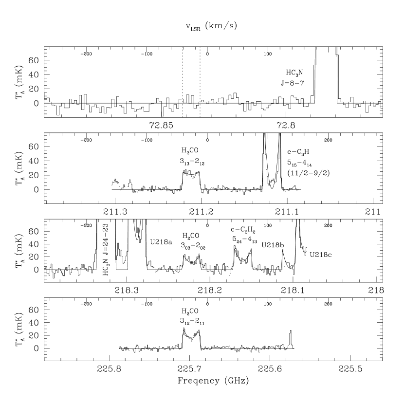
Figure 6: – Followup spectra at central position. This plot follows the conventions of Figure 1. The line parameters for the displayed fits can be found in Table 3. The dotted lines in the top panel indicate the expected position of the $1_{01}-0_{00}$ transition of formaldehyde (see text for further details).

We also conducted followup observations in early 2004 to detect additional lines of formaldehyde, also using the IRAM $30$m. We used the A230 and B230 receivers to observe the $3_{13}-2_{12}$, $3_{03}-2_{02}$ and $3_{12}-2_{11}$ transitions of formaldehyde, with rest frequencies of $211211.468$, $218222.192$, and $225697.775\,$MHz, respectively. We also used an experimental setup of the B100 receiver in an unsuccessful attempt to detect the $1_{01}-0_{00}$ transition of formaldehyde at a rest frequency of $72837.948$MHz. We again used the wobbler switching mode, with the same period and beam throw, and we used the same calibration procedures as for our initial observations. On each receiver, we used one $256\,$channel $1\,$MHz filterbank in parallel with the Vespa correlator system, set to a resolution of $320\,$kHz and a bandwidth of $160\,$MHz (100 GHz receiver) or $320\,$MHz (for the 230 GHz receivers). For all of our observations, lines were placed in the lower sideband (LSB). Data reduction was the same as for our initial observations, except as noted in discussions below. Our followup observation spectra are plotted in Figure 6 with line fits; we discuss each spectrum separately.

Our $72.838\,$GHz observations were conducted using a new receiver setup which involved tuning the B100 receiver to frequencies below the nominal limits of the system, and using the LO system from the B230 receiver. The spectrum plotted is from the $1\,$MHz filterbank. Owing to operational difficulties with the system, we obtained data at only one LO setting and we did not obtain a spectrum of the image band. The system was still undergoing commissioning tests during our observations and flux calibrations may not be entirely reliable. The single observed line in this spectrum, the HC₃N $J=8-7$ line, has been observed only once before, by Morris et al. (1975) and our observation is consistent with their flux measurements, but owing to the relatively large flux uncertainties of the Morris et al. (1975) observation, we are unable to obtain a better calibration, and estimate that our systematic uncertainty may be as high as $50\%$. The vertical dashed lines in this spectrum indicate the expected position of the $1_{01}-0_{00}$ transition of formaldehyde.

The spectrum plotted around $211.211\,$GHz represents data taken at two LO settings and is from the $1\,$MHz filterbank. The spectrum shows only two features. We identify the line at $v_{LSR}=-26.5\,{\rm km\,s^{-1}}$ as the $3_{13}-2_{12}$ transition of formaldehyde. The remaining feature is due to a blend of the $5_{15}-4_{14}$ $11/2-9/2$ $6-5$ and $5-4$ transitions of c-C₃H.

The $218.222\,$GHz spectrum was obtained using a wider bandwidth than the rest of our spectra. This spectrum was obtained using the VESPA correlator system and stretches from $218.084$ to $218.479\,$GHz (the portion which is not displayed contains no obvious features). The spectrum has been smoothed to a resolution of $1.25\,$MHz per channel to improve our signal to noise ratio. This spectrum represents only one LO setting, though we were able to obtain a spectrum of the image band. It confirms that the main features in the displayed spectrum are uncontaminated by features from the image band. There are 6 lines in this spectrum, only 3 of which can be identified. The largest feature, near $218.32\,$GHz is the $J=24-23$ transition of HC₃N. The next line, at around $218.29\,$GHz is unidentified, and we label it U218a. There does appear to be some non-zero flux between U218a and the HC₃N line; however, we are unable to associate it with a carrier or even a rough line fit so it is unlabelled. We identify the line near $218.22\,$GHz as the $3_{03}-2_{02}$ transition of formaldehyde. The line near $218.16\,$GHz is the $5_{24}-4_{13}$ transition of c-C₃H₂. The two line blend at the red edge of the spectrum consists of two unidentified lines, labelled U218b and U218c. In order to obtain reasonable line fits it was necessary to simultaneously fit U218b and U218c, and to constrain the expansion velocity of the fit for U218c. The $225.697\,$GHz spectrum shows only one line, the $3_{12}-2_{11}$ line of formaldehyde.

Given that we have carried out a very deep integration towards IRC+10216, it is worth considering the odds that we have misidentified the putative H₂CO lines due to confusion with previously uncataloged, unidentified lines, or U-lines. If we take as our null hypothesis that H₂CO is not responsible for any of the lines in any of our spectra, we find that there is one U-line in our $140.8\,$GHz spectrum, two in our $150.5\,$GHz spectrum, one in our $211.2\,$GHz spectrum, four in our $218.2\,$GHz spectrum, and one in our $225.7\,$GHz spectrum. We can then determine the probability that five of the nine U-lines should - by random chance - lie at the five H₂CO frequencies. This is the probability that our identification is in error.

Our bandwidth for each of these spectra is $256\,$MHz, except for the $218.2\,$GHz spectrum where it is $395\,$MHz. Our null hypothesis is that there are no formaldehyde lines in our spectra, and that the lines we have been identifying as formaldehyde are actually U-lines. The rate of occurence of U-lines in each spectrum is just the number of U-lines in that spectrum divided by the number of independent resolution elements within that band. For all spectra except the $218.2\,$GHz spectrum, the resolution elements are $1\,$MHz wide; for the $218.2\,$GHz spectrum, the resolution elements have been smoothed to $1.25\,$MHz wide. Since any line fit which has a central frequency within $\pm 0.5$ a resolution element of the laboratory formaldehyde frequency would likely be identified as a transition of formaldehyde, the probability that a single line would meet that criterion is $P=1/256,\>2/256,\>1/256,\>4/316,$ and $1/256$, respectively for the $140.8,\>150.5,\>211.2,\>218.2$ and $225.7\,$GHz spectra. Thus, the odds that we would simultaneously confuse five independent U-lines with the five observed transitions of formaldehyde is only $P=(1/256)(2/256)(1/256)(4/316)(1/256)\sim 5.9\times 10^{-12}$. Our confidence in this formaldehyde identification is strengthened by the fact that the ratio of line fluxes of the $2_{11}-1_{10}\>$ to $2_{12}-1_{11}\>$ transition is observed to be $0.58\pm 0.03$, in agreement with the predicted value of 0.56.

3 Discussion

3.1 Models for formaldehyde emission

We have constructed several models to predict the strength and spatial distribution of formaldehyde emission around IRC+10216. In order to predict the emission characteristics, we needed to determine both the expected spatial distribution of formaldehyde and the excitation conditions of the molecule. To determine the spatial distribution of formaldehyde, we were able to use a photodissociation model similar to that discussed for H₂O and OH in Ford et al. (2003). We assumed that formaldehyde could be either a parent molecule (outgassed directly from an icy nucleus, like H₂O) or a daughter product (created when some larger parent molecule was photodissociated, as with OH). We assumed that the vaporized molecule (either formaldehyde or its unidentified parent) is injected into the outflow at $100\,$AU (based on calculations by Ford & Neufeld, 2001), and that the vaporized molecule travels undisturbed through the outflow until it is photodissociated. If the assumed vaporizing molecule is not formaldehyde, the parent is photodissociated into formaldehyde, and the formaldehyde is also subsequently photodissociated. We assume a photodissociation rate of the form $\Gamma_{i}(A_{v})=2C_{i}G_{0}\exp(-\alpha_{i}A_{v}-\beta_{i}A_{v}^{2})\,{\rm s^{-1}},$ where $i$ represents either a parent molecule or H₂CO, $A_{v}$ is the depth in visual magnitudes and $C_{i}$, $\alpha_{i}$ and $\beta_{i}$ are the relevant photodissociation parameters for a cloud assumed to be spherical and uniformly illuminated from the exterior by the ISUV field. The factor $G_{0}$ represents the relative strength of the ISUV field and $G_{0}=1$ defines the average ISUV field (Draine, 1978). Since the hypothetical parent of formaldehyde is unknown, we do not have tight constraints on the values of $C_{p}$, $\alpha_{p}$ and $\beta_{p}$, the photodissociation parameters of the parent molecule. Based on the findings of Meier et al. (1993), we initially assumed that $C_{p}=C_{H_{2}CO}=7.81\times 10^{-10}\,$s^-1. We also assumed $\alpha_{p}=\alpha_{H_{2}CO}=2.22$ and $\beta_{p}=\beta_{H_{2}CO}=0.0$, since there are no observations which place useful constraints on these parameters. The values of the photodissocation parameters for H₂CO were determined using the method described in the appendix of Ford et al. (2003) based on plane-parallel parameters for H₂CO from Roberge et al. (1991). Under the assumption that the photodissociation parameters for the unknown formaldehyde parent molecule are identical to the parameters for formaldehyde, we can run a single model to determine the spatial distribution of formaldehyde as either a vaporizing molecule or daughter product. We plot the results of this calculation in the upper panel of Figure 8. The photodissociation model we used was the standard model, A, from Ford et al. (2003), that is, $G_{0}=1$, $A_{v}/N_{H}=5.6\times 10^{-22}\,{\rm mag\,cm^{2}}$ and $\dot{M}=3\times 10^{-5}\,{\rm M_{\odot}\,yr^{-1}}$.

Given a spatial distribution for the formaldehyde, we can calculate the excitation conditions of the molecule and the line strengths of various transitions. For these calculations, we employed the Large Velocity Gradient (LVG) code of Neufeld & Kaufman (1993). The LVG code uses the escape probability method to solve the equations of statistical equilibrium for the energy levels of formaldehyde. We used the same parameters for the circumstellar conditions as Melnick et al. (2001), listed here in Table 6. We obtained the formaldehyde Einstein-A coefficients and the energy levels from Jaruschewski et al. (1986), and the collisional coefficients from Green (1991). Given an assumed abundance and spatial distribution for formaldehyde, the LVG program calculates both the total line strength for various transitions, and (for each transition) the amount of line luminosity, $dL$, produced in a given radial interval, $dr$, as a function of $r$, where $r$ is the astrocentric radius. We have a third program which uses the tabulated $dL(r)/dr$ to calculate the formaldehyde line strength and shape after convolution with the telescope beam and Gaussian microturbulence. The IRAM 30m telescope has a frequency-dependent $HPBW$ of $17\arcsec$ at $140\,$GHz (near the $2_{12}-1_{11}\>$ transition of formaldehyde), $16\arcsec$ at $150\,$GHz (near the $2_{11}-1_{10}\>$ transition of formaldehyde) and $10\arcsec$ around $240\,$GHz. The convolution program is similar to the line shape program of Ford et al. (2003), except that this program also allows calculations of line strengths at offset positions. We can compare the output of the convolution program directly to our observations.

3.2 Comparison of models with observation

In comparing our models with our observations, we will rely primarily on the $150.498\,$GHz $2_{11}-1_{10}\>$ transition of formaldehyde, for reasons we detail below. In order to accurately determine the abundance of formaldehyde around IRC+10216, we must first determine its radial distribution, since any abundance determination will depend on the excitation conditions of formaldehyde, which in turn depends on formaldehyde’s radial distribution. Fortunately, our offset observations are ideally suited to distinguishing whether formaldehyde has a compact or extended source in IRC+10216. We find, based on our “average off-center position”, that the ratio of $(\int T_{A}^{*}dv)_{off}$, the integrated antenna temperature at the off-center position, to $(\int T_{A}^{*}dv)_{cent}$, the integrated antenna temperature at the central position is $0.40\pm 0.03$ at the $150.498\,$GHz $2_{11}-1_{10}\>$ transition and $0.51\pm 0.02$ at the $140.840\,$GHz $2_{12}-1_{11}\>$ transition. Here we are quoting statistical errors only ($1\sigma$), and we point out that the $2_{12}-1_{11}\>$ transition may be partly contaminated by the C₅H doublet. The contamination from the C₅H lines is likely to be higher in the off-center data, due to the increased relative strength of the doublet in our off-center spectrum. We therefore ignore the ratio for the $140.840\,$GHz $2_{12}-1_{11}\>$ transition, as we consider it to be unreliable, and concentrate on the ratio for the $150.498\,$GHz $2_{11}-1_{10}\>$ transition. We can compare this ratio to the predicted ratio obtained from line strengths calculated by our convolution program. We find, for widely varying formaldehyde abundances, $(\int T_{A}^{*}dv)_{off}/(\int T_{A}^{*}dv)_{cent}=0.09$ if formaldehyde is a parent molecule, or $(\int T_{A}^{*}dv)_{off}/(\int T_{A}^{*}dv)_{cent}=0.3$ if formaldehyde is a daughter molecule whose parent has identical photodissociation parameters to formaldehyde. We can obtain a best fit ratio, $(\int T_{A}^{*}dv)_{off}/(\int T_{A}^{*}dv)_{cent}=0.4$ for $C_{p}=1.6\times 10^{-10}\,$s^-1 (we still assume $\alpha_{p}=2.22$ and $\beta_{p}=0.0$, since our observations are not well suited to determining these parameters and these values for $\alpha$ and $\beta$ are fairly typical for a variety of molecules characterized by Roberge et al. (1991)). Clearly, formaldehyde has an extended source in the envelope of IRC+10216 and a parent molecule with the same photodissociation parameters as formaldehyde is not quite permitted by the data. We note that $C_{p}$ is not well constrained by our observations, as large variations in $C_{p}$ produce smaller variations in the ratio $(\int T_{A}^{*}dv)_{off}/(\int T_{A}^{*}dv)_{cent}$. We plot $C_{p}$ versus $(\int T_{A}^{*}dv)_{off}/(\int T_{A}^{*}dv)_{cent}$ in Figure 7. We also plot the spatial distribution of formaldehyde for our best fit $C_{p}$ in the bottom panel of Figure 8.

Based on our knowledge that formaldehyde has an extended source in the envelope around IRC+10216, and using the best fit photodissociation parameters for formaldehyde’s parent molecule, we can now determine the peak abundance of formaldehyde, relative to molecular hydrogen, which we find to be $x({\rm H_{2}CO})=1.3^{+1.5}_{-0.8}\times 10^{-8}$, assuming an ortho-to-para ratio of 3:1, as expected in LTE. As with water vapor, the abundance depends on the assumed stellar mass loss rate, and higher abundances correspond to lower mass loss rates. This abundance determination is based on the $2_{11}-1_{10}\>$ transition line strength only, as line blending produces systematic errors in the measured strength of the $2_{12}-1_{11}\>$ transition which are difficult to estimate; however, our models predict a line strength for the $2_{12}-1_{11}\>$ transition of $(\int T_{A}^{*}dv)_{2_{12}-1_{11}}=701\pm 37\,{\rm mK}{\rm\,km\,s^{-1}},\>(1\sigma)$ for the abundance range quoted above. These predicted fluxes are quite consistent with the measured value of $(\int T_{A}^{*}dv)_{2_{12}-1_{11}}=687\pm 19\,{\rm mK}{\rm\,km\,s^{-1}},\>(1\sigma)$. In addition, the measured relative strengths of the formaldehyde lines are in good agreement with the relative strengths predicted by our LVG excitation code.

In contrast with our 2mm observations, the lines detected in our followup observations are stronger than predicted by factors of $\sim 3-8$. We believe these discrepancies can be attributed to the molecular collision rate coefficients we used in our LVG code, specifically those computed by Green (1991). These collision rates were computed for collisions of formaldehyde with atomic helium, while in the circumstellar envelope of IRC+10216 (and in most other astrophysical instances) the dominant collision partner will be molecular hydrogen. The use of atomic helium as a substitute partner in collision models is nevertheless routine, due to the fact that the potential of atomic helium is vastly simpler to deal with computationally than the potential of molecular hydrogen, thus enabling the calculation of collision rates for a fairly large selection of molecules in a reasonable amount of time. As suggested by Green (1991), in order to use the H₂CO-He collision rates for H₂CO-H₂ collisions we applied a uniform correction factor ($2.2$) to the H₂CO-He collision rates to account for the difference in the cross-sections and relative collision velocities of He and H₂. However, Green (1991) also notes there is likely some variation in the detailed state to state collision rates owing to the detailed differences between the He and H₂ potentials. Specifically, ammonia is one of the few molecules for which both He and H₂ collision rates have been calculated and comparisons with the findings of those studies are instructive. In the case of ammonia collisions, it was found that for transitions where $\Delta J>1$, rotationally excited H₂ caused transition rates to be enhanced by a factor of $2-3$. Additionally, even for excitation by H${}_{2}(j=0)$ rates were usually only within a factor of 2 of the rates for excitation by He, though some were larger and some were smaller, with no obvious pattern. The analysis of our observations is thus severely impeded by the lack of reliable collision rates; however, since the $J=3-2$ transitions (i.e. all of the 1.3mm line detections) would be preferentially affected by enhancements of collision rates for $\Delta J>1$ transitions, we regard these lines as less reliable indicators of the formaldehyde abundance in IRC+10216 and we do not rely on them for our abundance estimate. Given the uncertainties in all of our collision rates, we must be cautious in interpreting our calculated abundances. While we consider the 2mm transitions to be the most reliable abundance indicators, even they may lead to abundance estimates which are off by factors of $2$ or possibly more.

Another discrepancy between our predictions and observations is posed by our non-detection of formaldehyde at $72.838\,$GHz, where the $3\sigma$ upper limit is weaker than the line strength predicted by our standard model by a factor of about $1.8$. While collision rates may play a role here, we believe the overprediction can be primarily attributed to two effects: 1) the uncertain calibration of observations at this frequency (possibly up to $\sim 50\%$ and 2) the sensitivity of this transition to the size of the emitting region. Due to the low frequency of these observations, the $72.838\,$GHz line was subject to the largest beamsize of any of our observations. If the UV field was slightly stronger than we assumed, or the unshielded photodissociation rate of formaldehyde (which we estimate to be accurate to no better than $20\%$) was slightly larger than we assumed, the size of the formaldehyde emitting region would shrink somewhat, and the predicted flux at $72.838\,$GHz would drop, while the flux for higher frequency lines would remain unaffected. Since we were unable to detect the $1_{01}-0_{00}$ transition at $72.838\,$GHz, our only detected transition of para-H₂CO is the $3_{03}-2_{02}$ transition; in the absence of more reliable collision rates we believe we cannot accurately model the excitation of this transition and cannot rely on it to determine the ortho:para ratio of H₂CO in this source. Since our models of the $1_{01}-0_{00}$ transition are likely the more reliable of the two para-H₂CO lines, we find that our observations are not inconsistent with the LTE ortho:para ratio of 3:1, which we therefore assume throughout this paper.

Despite the uncertainties, our determined abundance agrees well with measured values of the formaldehyde abundance relative to water vapor in Solar System comets. If we take $x({\rm H_{2}O})=(4-27)\times 10^{-7}$ around IRC+10216, our peak formaldehyde abundance with respect to water is $x({\rm H_{2}CO})/x({\rm H_{2}O})=(1.1\pm 0.2)\times 10^{-2}$. The fractional error on the relative abundance of formaldehyde to water vapor is much smaller than the error on either the water vapor abundance or the formaldehyde abundance because the primary source of error in the absolute abundance measurements is the stellar mass loss rate, and this affects both absolute abundances similarly, so the error tends to cancel out, allowing us to determine the relative abundance very precisely. This compares well with the peak values measured for Comet Lee ($x({\rm H_{2}CO})/x({\rm H_{2}O})=1\times 10^{-2}$) (Biver et al., 2000), Comet Hyakutake ($x({\rm H_{2}CO})/x({\rm H_{2}O})=8\times 10^{-3}$) (Biver et al., 1999) and several comets observed by Colom et al. (1992) ($x({\rm H_{2}CO})/x({\rm H_{2}O})\sim 5\times 10^{-3}$).

While we do not know the identity of the carrier of U150, we can also use our photodissociation model to make some useful statements about possible carriers of the U150 line. The carrier of the U150 line is likely to be a product of the rich photochemistry in the circumstellar envelope of IRC+10216. The line has a high off-center/central-position ratio, comparable to or greater than the off-center/central-position ratio of the formaldehyde line in the $150\,$GHz band, indicating that the carrier is at least as extended as formaldehyde. We can obtain additional information about the spatial distribution of the U150 line carrier by examining its line shape in our central and off-center spectra. The U150 line has a double-peaked profile in our central position observations, indicating a resolved source, i.e. the emission is much larger than the telescope beam ($HPBW=16\arcsec$). By contrast, the off-center line shape for U150 is relatively flat-topped, particularly compared to the c-C₃H₂ line, as would be expected for a source which is less extended than the c-C₃H₂ line. This conclusion is supported by the off-center/central-position ratio for the c-C₃H₂ line, which is larger than for the U150 line. In addition, the existence of relatively bright emission in U150 so far from IRC+10216 indicates that the line originates in a relatively low-lying state which is easily excited even at the lower densities found beyond $\sim 1400\,$AU from the star.

3.3 Chemical production of formaldehyde?

A recent paper by Willacy (2004) has suggested that the water vapor and OH found around IRC+10216 could be formed chemically by Fischer-Tropsch catalysis on grain surfaces. While this mechanism is incapable of directly producing large amounts of formaldehyde (comparable to what we see in IRC+10216), Willacy suggests that the presence of formaldehyde could be explained separately by the photodissociation of methanol, which could be formed in large quantities by Fischer-Tropsch reactions. Our failure to detect methanol in significant quantities rules out this method of production of formaldehyde, and also suggests that grain catalysis is not the source of the water vapor and OH around IRC+10216. Nevertheless, there are plausible chemical production routes for formaldehyde which we examine here. There are at least two important reactions that are responsible for the production of formaldehyde around oxygen-rich asymptotic giant branch stars, which may also operate around IRC+10216. These are

$${\rm OH}+{\rm CH_{2}}\to{\rm H_{2}CO}+{\rm H}$$ (1)

and

$${\rm O}+{\rm CH_{3}}\to{\rm H_{2}CO}+{\rm H}.$$ (2)

In both oxygen-rich stars and in IRC+10216, the CH₂ and CH₃ would be produced by the photodissociation of methane (CH₄). The source of OH around IRC+10216 and oxygen-rich stars would also be the same, namely the photodissociation of water vapor. The atomic oxygen required for the second reaction would come almost exclusively from the photodissociation of CO in the case of IRC+10216, but for oxygen-rich stars, both the CO and OH will make a contribution. In both types of stars atomic oxygen will be available in the outermost regions of the circumstellar envelope. Clearly then, the reactants are available around IRC+10216, and since they are themselves photodissociation products, they will result in an extended source for formaldehyde, consistent with our observations. We must therefore calculate if chemical reactions will produce enough formaldehyde to match our observations.

A rough estimate of the expected formaldehyde abundance may be made by comparing the methane and water vapor abundances around IRC+10216 to that around oxygen-rich stars. Willacy & Millar (1997) have modeled the chemistry of several oxygen-rich stars, including the reactions listed above for creating formaldehyde. They typically find, for assumed abundances of $x({\rm H_{2}O})=3\times 10^{-4}$ and $x({\rm CH_{4}})=3\times 10^{-5}$, a peak formaldehyde abundance of $x({\rm H_{2}CO})\sim 10^{-6}$. Since the observed $x({\rm H_{2}O})$ and $x({\rm CH_{4}})$ for IRC+10216 are down by factors of $\sim 300$ (Melnick et al., 2001) and $\sim 10$ (Keady & Ridgway, 1993), respectively, and because $x({\rm H_{2}CO})$ is dependent on the product of $x({\rm H_{2}O})$ and $x({\rm CH_{4}})$, we expect $x({\rm H_{2}CO})$ to be down by a factor of roughly 3000 relative to the models of Willacy & Millar (1997), or $x({\rm H_{2}CO})\sim 3\times 10^{-10}$. This is about 2 orders of magnitude less than is observed in IRC+10216, which does not make the chemical explanation look very promising. We can also do a more careful calculation, modeling the individual chemical reactions which produce formaldehyde. Models by Petrie, Millar & Markwick (2003) tabulate the abundances of CH₂, CH₃ and atomic oxygen as a function of radial distance from IRC+10216, and we have a model from Ford et al. (2003) which tabulates the abundance of OH as a function of radius. If we assume that the creation of formaldehyde is a perturbation to these abundances (i.e. the reaction does not consume large quantities of any of the reactants), we can simply model the abundance of formaldehyde as a function of radius with the equation

$$\dot{x}({\rm H_{2}CO})=k_{1}n_{\rm H_{2}}x({\rm OH})x({\rm CH_{2}})+k_{2}n_{\rm H_{2}}x({\rm O})x({\rm CH_{3}})-\Gamma_{\rm H_{2}CO}x({\rm H_{2}CO}).$$ (3)

Here $\dot{x}({\rm H_{2}CO})$ is the time derivative of $x({\rm H_{2}CO})$, where time and radius are related through the expression $R=v_{exp}t$, $n_{\rm H_{2}}$ is the density of molecular hydrogen, $k_{1}=3.0\times 10^{-11}$ and $k_{2}=1.3\times 10^{-10}$ are the appropriate reaction rates in units of cm${}^{3}\,$s^-1 (Le Teuff, Millar & Markwick, 2000) and $\Gamma_{\rm H_{2}CO}$ is the photodissociation rate of formaldehyde. Our calculation is slightly complicated by the fact that the H₂O abundance, and therefore the OH abundance, is somewhat uncertain. But we can easily calculate the expected abundance of formaldehyde with respect to water vapor, $x({\rm H_{2}CO})/x({\rm H_{2}O})$, by simply dividing our calculated $x({\rm H_{2}CO})$ by our assumed $x({\rm H_{2}O})$. Integrating equation 3, and assuming $x({\rm H_{2}O})=1.2\times 10^{-6}$, we find a peak formaldehyde abundance of $x({\rm H_{2}CO})=1.1\times 10^{-9}$, which is slightly larger than our rough estimate, but still an order of magnitude smaller than our observed value. Importantly, we find that for all plausible values of $x({\rm H_{2}O})$, chemical reactions can only produce $x({\rm H_{2}CO})/x({\rm H_{2}O})\sim 0.1\%$, or about an order of magnitude less than our observed ratio. We plot the spatial distribution of chemically produced formaldehyde, as well as the relevant reactants in Figure 9, for $x({\rm H_{2}O})=1.2\times 10^{-6}$. We note here that if we were to treat the problem not as a perturbation to the chemistry, but were to allow the formaldehyde reaction to consume reactants, this would further depress the calculated $x({\rm H_{2}CO})$. In view of these calculations, we believe we can safely rule out any chemical explanation for the presence of formaldehyde around IRC+10216.

3.4 Hints of asymmetry?

The mapping observations we obtained contain tantalizing hints that the distribution of formaldehyde around IRC+10216 is not spherically symmetric. If we look at the off-center data separately by position angle (as opposed to the “average off-center position” we discussed above), we see that a positive signal was detected at both $140.840$ and $150.498\,$GHz at all positions, though several of the positions have signals that are not statistically significant (see Table 4). We have plotted the data from Table 4 for the H₂CO $2_{11}-1_{10}$, c-C₃H₂ $2_{20}-1_{11}$ and SiC₂ $6_{25}-5_{24}$ lines, with the line strengths normalized relative to the average line strength at each frequency, in Figure 10 (we ignore the H₂CO $2_{12}-1_{11}\>$ data due to sytematic errors from line blending which are difficult to eliminate). The c-C₃H₂ $2_{20}-1_{11}$ and SiC₂ $6_{25}-5_{24}$ lines are our “control lines”, since c-C₃H₂ and SiC₂ are molecules that are produced normally in a carbon-rich circumstellar envelope. These molecules should be entirely unrelated to the vaporizing Kuiper Belt analog. Additionally, our control lines were bright, unblended and do not contain any bad channels, so we believe that the systematic errors associated with the measured line strengths will be neglible. We can see that the line strengths of the control lines do not vary much with position angle. By contrast, the formaldehyde line varies substantially, in one case, at position angle $210^{\circ}$, by more than $3\sigma$ from the average value. Since there are $8$ data points, the probability of such a large variation occurring by random chance at any $1$ of the $8$ points is $4\times 10^{-3}$, but this still represents an exciting hint that formaldehyde may have a different spatial distribution than other molecules with well-understood formation mechanisms in the circumstellar envelope of IRC+10216 (based on our two control lines). We expect that formaldehyde would have a spatial distribution independent of these other “native” molecules if the formaldehyde were produced by outgassing from a Kuiper Belt analog; in that case, we would still expect the spatial distribution of formaldehyde to track that of water vapor and OH. We have a very poor idea of the spatial distribution of either the water vapor or the OH, though, as discussed previously, the OH may show signs of being asymmetrically distributed. One natural model for the spatial distribution of all three of these molecules is, of course, a disk or ring structure, which would display departures from circular symmetry if we observed the ring more or less edge-on. If we observe an essentially edge-on ring, we would expect our data to show evidence of periodicity, with a period of $180^{\circ}$. There does not appear to be an elevated signal $180^{\circ}$ away from the elevated point at $210^{\circ}$, as would have been expected for an edge-on system; however, at the present signal to noise level, it is difficult to rule out a ring with any certainty.

Our tentative hints of asymmetry in the distribution of formaldehyde are especially interesting in light of OH observations by Ford et al. (2003). We believe that both the OH and formaldehyde are photodissociation products of parent molecules which are released from cometary nuclei in orbit around IRC+10216. Therefore, we might expect H₂CO and OH to have similar spatial distributions and line shapes. Instead, OH and H₂CO possess very different line shapes, indicating different spatial distributions. We do not fully understand why OH displays a narrow, blue-shifted line profile, and like Ford et al. (2003), we believe that the spatial distribution of OH around IRC+10216 requires further study. We can think of no production mechanism for H₂CO in the envelope of IRC+10216 that is not closely related to OH; we are therefore at a loss to explain the clearly differing line shapes. In addition, the possible asymmetries noted in the OH and formaldehyde distributions are not the same – OH has a front-to-back asymmetry, while formaldehyde’s asymmetry is in the plane of the sky (if it exists at all). Also, formaldehyde does not appear to be substantially asymmetrically distributed in the inner regions of the outflow around IRC+10216, as evidenced by the shapes of the formaldehyde lines in our central position observations. Unfortunately, we do not have similar information on the spatial distribution of OH, since Arecibo has a much larger beam than IRAM, and we do not have mapping observations of the OH from Arecibo. Clearly these discrepancies require further study – ideally, deep maps of the distribution of both formaldehyde and OH. Further mapping observations of formaldehyde around IRC+10216 should be not be difficult or enormously time consuming, and such maps will determine if the hints of formaldehyde’s asymmetry are real. Mapping of OH around IRC+10216, on the other hand, would consume large amounts of telescope time, due to the faint OH signal (sure to become fainter for off-center observations). Still, we view this as an extremely interesting and important observation, and it may be possible to complete an OH mapping campaign without placing undue demands on telescope time if the campaign were stretched over several observing seasons.

3.5 Methanol

If we believe that the formaldehyde around IRC+10216 is produced by vaporization from icy bodies with chemical compositions similar to Solar System comets, we would also expect to detect methanol in substantial quantities. Methanol is usually present in Solar System comets at the few percent level (relative to water vapor) (Bockelée-Morvan, 1996). In individual comets, methanol is usually observed to be more abundant than formaldehyde (see Colom et al., 1992; Biver et al., 1999, 2000; Ehrenfreund & Charnley, 2000, and references therein). Ices in Solar System comets, in turn, are believed to come from the interstellar medium, and are expected to have a similar chemical composition to interstellar ices, particularly those found in molecular hot cores (Ehrenfreund & Charnley, 2000). Indeed, both the methanol and formaldehyde found in comets is believed to form from grain surface reactions in the ISM, through successive hydrogenation reactions with CO. Observations of hot cores indicate that their methanol abundances can vary widely, with methanol ice abundances as high as $30\%$ relative to water ice in some sources, and upper limits in other sources as low as $2\%$ (Dartois et al., 1999). Very small abundances of methanol are difficult to measure in the ice phase, due to the fact that the spectral features for solids are broad and difficult to distinguish at low abundance.

Our expected line strengths for methanol were based on models kindly run by Silvia Leurini (private communication), using collision rates from Pottage, Flower & Davis (2001, 2002). Our observations could have detected methanol lines as faint as $T_{A}^{*}>10\,{\rm mK}\,(3\sigma)$. Models by S. L. indicate that the brightest line in our band would be the $5_{00}-4_{00}$ transition of the A species of methanol at $241791.3\,$MHz, and we could have detected this line of methanol at abundances as small as $x({\rm CH_{3}OH})>8.5\times 10^{-10}\,(3\sigma)$ or $x({\rm CH_{3}OH})/x({\rm H_{2}O})<7.7\times 10^{-4}$. Our non-detection therefore requires some explanation, if we believe the formaldehyde comes from comet-like bodies. One possible explanation is that the methanol is being pumped by the large IR luminosity of IRC+10216 into vibrationally excited states, and the transitions between low-lying states we attempted to observe are substantially fainter than expected due to depopulation of the low-lying states; however, a full excitation calculation including IR pumping is beyond the scope of this paper (and is also not presently available from S. L.). Another possible explanation is that there is no methanol at all, or at least that it is substantially underabundant, compared with methanol in normal Solar System comets. This could simply be the result of different chemistry in the natal cloud of IRC+10216 (as compared with our Solar System), which resulted in a depletion of methanol for Kuiper Belt Object (KBO) analogs that formed around IRC+10216. This is not entirely implausible, considering the wide range of observed methanol abundances in star forming regions (molecular hot cores). It is also possible that comets around IRC+10216 are more similar to a special class of comets, which, in our Solar System are relatively rare. There exists a class of comets which are methanol-poor ($x({\rm CH_{3}OH})/x({\rm H_{2}O})<0.17\%$), but which have essentially normal formaldehyde abundances (Mumma et al., 2002). It is not understood how these comets became methanol-depleted in our own Solar System, so we are truly at a loss to explain why most comets in another system would be so methanol-poor. Further study of methanol-poor comets in the Solar System is clearly warranted.

3.6 Al³⁷Cl

We have analysed the observed strength of the Al³⁷Cl $J=17-16$ line using an excitation model similar to that used to interpret observations of formaldehyde and water vapor (Melnick et al., 2001). For the case of AlCl, our analysis is hindered by a lack of reliable molecular data. As far as we are aware, rate coefficients have never been computed for collisional excitation of AlCl, and the dipole moment (1–2 Debye, according to measurements of the Stark effect by Lide, 1965) remains uncertain by a factor of 2. Accordingly, we simply used rate coefficients for excitation of CO by H₂ in place of those for excitation of AlCl, and assumed a dipole moment of 1.5 Debye in computing the spontaneous radiative decay rates. Fortunately, the predicted line fluxes are very insensitive to the assumed rate coefficients for collisional excitation; they are, however, roughly proportional to the square of the assumed dipole moment. Predicted line fluxes have been corrected assuming a frequency dependent telescope beamsize of $HPBW=10\arcsec$ at $240\,$GHz.

A best fit to the available measurements of millimeter-wave line emission from Al³⁷Cl and Al³⁵Cl is obtained for a total assumed AlCl abundance of $4\times 10^{-8}$ relative to H₂ and an assumed Al³⁵Cl/Al³⁷Cl abundance ratio of 3. In Figure 11, we show the integrated line fluxes observed for Al³⁵Cl and Al³⁷Cl as function of $J_{u}$, the rotational quantum number of the upper state. Open symbols apply to Al³⁵Cl and filled symbols to Al³⁷Cl. Squares show the line strengths reported in the AlCl discovery paper of Cernicharo & Guélin (1987) and the 2mm line survey of Cernicharo et al. (2000; results for the $J=12-11$ line of Al³⁷Cl are excluded because that line is severely blended); and the filled circle shows the Al³⁷Cl $J=17-16$ flux reported here. The dashed and solid curves, respectively, show the model predictions for Al³⁵Cl and Al³⁷Cl, obtained for a total assumed AlCl abundance of $4\times 10^{-8}$ relative to H₂ and an assumed Al³⁵Cl/Al³⁷Cl abundance ratio of 3.

Figure 11 demonstrates that an acceptable fit can be obtained for Al³⁷Cl $J=17-16$ line that is broadly consistent with the lower-frequency transitions detected previously, lending support to our line identification. The inferred total AlCl abundance of $4\times 10^{-8}$ relative to H₂ amounts to 8% of the solar abundance of Cl (Anders & Grevesse, 1989) and 0.6% of the solar abundance of Al. Because the derived AlCl abundance is inversely proportional to the square of the assumed dipole moment, it is uncertain by at least a factor of 2. Our value for the AlCl abundance is in broad agreement with that found by Highberger et al. (2003), as well as with the photospheric AlCl abundances predicted by models of cool stellar atmospheres (e.g. Tsuji, 1973).

4 Conclusions

We have clearly detected formaldehyde around the carbon-rich AGB star IRC+10216, and demonstrated that formaldehyde has an extended source in the circumstellar envelope around IRC+10216. The formaldehyde around IRC+10216 is present at a level of around $1\%$, relative to water vapor, consistent with formaldehyde abundances in Solar System comets. Our observations, combined with previous work by Melnick et al. (2001) and Ford et al. (2003) lead us to conclude that formaldehyde is a molecule produced by the photodissociation of an unknown parent molecule, and that the parent molecule is produced by vaporization from the surfaces of cometary nuclei orbiting IRC+10216 in a Kuiper Belt analog. We did not detect methanol around IRC+10216, despite our deep search, and our upper limits on the methanol abundance ($<0.077\%$ relative to water vapor) imply that any cometary system around IRC+10216 contains significantly less methanol than typical Solar System comets.

Chemical characterization of extrasolar cometary systems is important for a variety of reasons. The chemical composition of cometary systems can tell us something about the conditions in protoplanetary disks around forming stars, and therefore can provide us with interesting information on the process of star formation. The study of extrasolar cometary systems also bears directly on the emerging field of astrobiology (Ehrenfreund & Charnley, 2000; Oró, Miller & Lazcano, 1990). In our own Solar System, it is believed that much of the volatile carbon present on the young Earth was delivered by comets (Chyba & Sagan, 1992). Comets contributed volatile carbon both in the form of simple molecules like formaldehyde and methanol and as more complex molecules like amino acids (Anders, 1989; Chyba, 1990; Pierazzo & Chyba, 1999). It has been suggested (Cronin & Chang, 1993; Oró & Lazcano, 1997) that this extraterrestrial volatile carbon contribution formed the basis of the pre-biotic carbon chemistry which led to the formation of extremely complex molecules and eventually to single-celled organisms and all life on Earth. Thus, the chemistry of extrasolar cometary systems may have important consequences for the probability of life forming on otherwise habitable exoplanets. Ultimately, we would like to survey the chemical composition of a large number of extrasolar cometary systems and compare their compositions to the chemical composition of Solar System comets.

Table 1: Oxygen-bearing Molecules in Comets

Molecule	Abundance Range
H2O	$100.$
CO	$5.-80.$
CO2	$3.-30.$
CH3OH	$1.-7.$
H2CO	$0.05-4.$
OCS	$0.3$
SO2	$\leq 0.001$

Note. — Abundances of oxygen-bearing molecules detected in Solar System comet comae, listed as a percentage, relative to water. From Bockelée-Morvan (1996).

Table 2: Integration Times

Position	Frequency Band (GHz)	Time (minutes)
center	73	134
center	141	1166
center	150	976
center	211	312
center	218	232
center	226	436
center	242	2452
off-center, 30°	141	128
off-center, 75°	141	124
off-center, 120°	141	128
off-center, 165°	141	124
off-center, 210°	141	128
off-center, 255°	141	122
off-center, 300°	141	128
off-center, 345°	141	120
off-center, 30°	150	328
off-center, 75°	150	124
off-center, 120°	150	332
off-center, 165°	150	124
off-center, 210°	150	328
off-center, 255°	150	122
off-center, 300°	150	328
off-center, 345°	150	120
off-center, avg.	141	1002
off-center, avg.	150	1726
off-center, avg.	242	2636

Note. — Times listed are on-source plus off-source.

Table 3: Line Fit Parameters

Species	$\nu_{rest}$	$\nu_{obs}$	Line Strength	$v_{exp}$
and Transition	(MHz)	(MHz)	(mK km s-1)	(km s-1)
HC3N $J=8-7$	72783.8220	72783.8 $\pm$ 0.5	67138 $\pm$ 82	14.0 $\pm$ 1.0
H2CO $1_{01}-0_{00}$	72837.9480	$\cdots$	$<246,3\sigma$	$\cdots$
C5H ${}^{2}\Pi_{1/2}\>J=59/2-57/2\,a$	140824.640	fixed	294 $\pm$ 19	14.5 (fixed)
C5H ${}^{2}\Pi_{1/2}\>J=59/2-57/2\,b$	140833.469	fixed	294 $\pm$ 19	14.5 (fixed)
H2CO $2_{12}-1_{11}$	140839.5020	fixed	687 $\pm$ 19	14.5 (fixed)
NaCN $9_{37}-8_{36}$	140853.858	fixed	704 $\pm$ 19	14.5 (fixed)
SiC2 $6_{25}-5_{24}$	140920.1478	140920.3 $\pm$ 0.5	34751 $\pm$ 19	14.6 $\pm$ 0.2
NaCN $9_{36}-8_{35}$	140937.428	fixed	679 $\pm$ 19	14.5 (fixed)
30SiC2 $6_{24}-5_{23}$	140955.918	140955.4 $\pm$ 0.5	1383 $\pm$ 25	14.9 $\pm$ 0.2
U150	$\cdots$	150385.9 $\pm$ 0.5	1040 $\pm$ 21	14.3 $\pm$ 0.2
c-C3H2 $2_{20}-1_{11}$	150436.5448	150436.5 $\pm$ 0.5	1049 $\pm$ 21	14.2 $\pm$ 0.2
H2CO $2_{11}-1_{10}$	150498.3340	150498.6 $\pm$ 0.5	396 $\pm$ 21	13.9 $\pm$ 0.2
c-C3H $5_{15}-4_{14}(11/2-9/2)6-5$	211117.5764	211117.6 $\pm$ 0.5	1132 $\pm$ 17	14.7 $\pm$ 0.3
c-C3H $5_{15}-4_{14}(11/2-9/2)5-4$	211117.8341	$\cdots$	$\cdots$	$\cdots$
H2CO $3_{13}-2_{12}$	211211.4680	211211.5 $\pm$ 0.5	652 $\pm$ 17	14.6 $\pm$ 0.3
U218c	$\cdots$	218085.8 $\pm$ 0.75	1734 $\pm$ 31	14.5 (fixed)
U218b	$\cdots$	218103.1 $\pm$ 0.75	353 $\pm$ 31	14.1 $\pm$ 0.4
c-C3H2 $5_{24}-4_{13}$	218160.4423	218160.2 $\pm$ 0.75	625 $\pm$ 31	15.0 $\pm$ 0.4
H2CO $3_{03}-2_{02}$	218222.1920	218222.0 $\pm$ 0.75	450 $\pm$ 31	14.3 $\pm$ 0.4
U218a	$\cdots$	218287.3 $\pm$ 0.75	3180 $\pm$ 31	14.4 $\pm$ 0.4
HC3N $J=24-23$	218324.7880	218324.7 $\pm$ 0.75	13976 $\pm$ 31	14.2 $\pm$ 0.4
H2CO $3_{12}-2_{11}$	225697.7750	225697.8 $\pm$ 0.5	598 $\pm$ 15	14.2 $\pm$ 0.3
Al37Cl $J=17-16$	241855.0339	241855.06 $\pm$ 0.3	1440 $\pm$ 16	14.0 $\pm$ 0.1

Note. — We list the line fit parameters for spectra displayed in Figures 1 and 6, and the ³⁰SiC₂ $6_{24}-5_{23}$ line. The ³⁰SiC₂ line was near the edge of our band at our first local oscillator setting and but was out of the band at our second local oscillator setting, thus, it received a bit more than half the integration time that other lines in that band received (resulting in somewhat higher noise levels), and it does not appear in the final spectrum displayed in Figure 1. Observed frequencies have been corrected for source motion, assuming a systemic velocity of $v_{LSR}=-26.5{\rm\,km\,s^{-1}}$. It is important to note that the errors listed in this table represent only the statistical errors ($1\sigma$) associated with each measurement; in several cases, systematic errors are more important than the statistical errors, and we estimate that the line strengths for lines with blends or bad channels may be uncertain by up to $50\%$.

Table 4: Off-Center Integrated Line Strengths in ${\rm mK\,km\,s^{-1}}$ as a Function of Position Angle

Position	H2CO	c-C3H2	SiC2	H2CO
Angle	$2_{11}-1_{10}$	$2_{20}-1_{11}$	$6_{25}-5_{24}$	$2_{12}-1_{11}$
30∘	153 $\pm$ 25	631 $\pm$ 25	18681 $\pm$ 27	371 $\pm$ 27
75∘	118 $\pm$ 88	779 $\pm$ 88	19661 $\pm$ 40	503 $\pm$ 40
120∘	138 $\pm$ 23	688 $\pm$ 23	18664 $\pm$ 30	522 $\pm$ 30
165∘	80 $\pm$ 55	678 $\pm$ 55	14449 $\pm$ 41	476 $\pm$ 41
210∘	216 $\pm$ 23	626 $\pm$ 23	14795 $\pm$ 27	515 $\pm$ 27
255∘	77 $\pm$ 53	788 $\pm$ 53	14882 $\pm$ 43	482 $\pm$ 43
300∘	124 $\pm$ 25	676 $\pm$ 25	14211 $\pm$ 31	311 $\pm$ 31
345∘	165 $\pm$ 56	756 $\pm$ 56	19737 $\pm$ 36	566 $\pm$ 36

Note. — We list the line strengths for spectra displayed in Figures 3 and 4. All line strengths are in units of mK km s^-1 and errors are $1\sigma$. Data for the H₂CO $2_{11}-1_{10}$, c-C₃H₂ $2_{20}-1_{11}$ and SiC₂ $6_{25}-5_{24}$ transitions are also plotted (in normalized units) in Figure 10.

Table 5: Off-Center Integrated Line Strengths Relative to Central Position Integrated Line Strengths

Species	$\nu_{obs}$	$(\int T_{A}^{*}dv)_{off}$	$v_{exp}$	$(\int T_{A}^{*}dv)_{off}/$
and Transition	(MHz)	(mK km s-1)	(${\rm km\,s^{-1}}$)	$(\int T_{A}^{*}dv)_{cent}$
C5H ${}^{2}\Pi_{1/2}\>J=59/2-57/2\,a$	140824.6 $\pm$ fixed	233 $\pm$ 13	13.6 $\pm$ fixed	0.79 $\pm$ 0.07
C5H ${}^{2}\Pi_{1/2}\>J=59/2-57/2\,b$	140833.5 $\pm$ fixed	233 $\pm$ 13	13.6 $\pm$ fixed	0.79 $\pm$ 0.07
H2CO $2_{12}-1_{11}$	140839.5 $\pm$ fixed	353 $\pm$ 13	13.6 $\pm$ fixed	0.51 $\pm$ 0.02
NaCN $9_{37}-8_{36}$	140853.9 $\pm$ fixed	203 $\pm$ 13	13.6 $\pm$ fixed	0.29 $\pm$ 0.02
SiC2 $6_{25}-5_{24}$	140920.0 $\pm$ 0.01	17684 $\pm$ 13	13.6 $\pm$ 0.02	0.5089 $\pm$ 0.0005
NaCN $9_{36}-8_{35}$	140937.4 $\pm$ fixed	177 $\pm$ 13	13.6 $\pm$ fixed	0.26 $\pm$ 0.02
30SiC2 $6_{24}-5_{23}$	140955.0 $\pm$ 1.0	678 $\pm$ 13	13.8 $\pm$ 2.0	0.49 $\pm$ 0.01
U150	150385.5 $\pm$ 0.3	473 $\pm$ 10	12.5 $\pm$ 0.5	0.46 $\pm$ 0.01
c-C3H2 $2_{20}-1_{11}$	150436.2 $\pm$ 0.1	698 $\pm$ 10	12.9 $\pm$ 0.2	0.67 $\pm$ 0.02
H2CO $2_{11}-1_{10}$	150497.9 $\pm$ 1.0	157 $\pm$ 10	13.5 $\pm$ 1.2	0.40 $\pm$ 0.03
Al37Cl $J=17-16$	241854.0 $\pm$ 0.2	116 $\pm$ 12	13.4 $\pm$ 0.3	0.081 $\pm$ 0.008

Note. — We list the line strengths for spectra displayed in Figure 5. Observed frequencies have been corrected for source motion, assuming a systemic velocity of $v_{LSR}=-26.5{\rm\,km\,s^{-1}}$. As in Table 3, we list only statistical errors ($1\sigma$); as in our central position observations, systematic errors may be quite large for blended lines or those with bad channels. We also calculate the ratio $(\int T_{A}^{*}dv)_{off}/(\int T_{A}^{*}dv)_{cent}$ for each line, based on the central position line strengths listed in Table 3. The errors quoted for the ratios are also only statistical.

Table 6: Excitation Model Parameters

Physical Conditions	Value Adopted
Dust shell inner radius, $R_{i}$	$2.58\times 10^{14}\,$cm
Dust shell outer radius	$1\times 10^{17}\,$cm
Outflow velocity, $v_{out}$	$14.5[1.00-0.95(R_{i}/r)]^{0.5}{\rm\,km\,s^{-1}}$
Turbulent velocity	$0.65{\rm\,km\,s^{-1}}$
H2 density	$(3.11\times 10^{7}\,{\rm cm^{-3}}/R_{15}^{2})\times(\dot{M}/3\times 10^{-5})\times(14.5/v_{out})$
Gas temperature	Max[$10,12(90/R_{15})^{0.72}$] K
Assumed distance, $D$	$170\,$pc

Figure 1: – Central position spectra showing formaldehyde detection. Plotted frequencies represent the frequency in the rest frame of the source (IRC+10216) assuming a systemic velocity of $v_{LSR}=-26.5{\rm\,km\,s^{-1}}$. Frequencies are plotted along the bottom axis, while $v_{LSR}$ is plotted along the top axis, with $v_{LSR}=-26.5{\rm\,km\,s^{-1}}$ centered on the frequency of interest – $140.840\,$GHz in the top two panels, $150.498\,$GHz in the next panel, and $241.791\,$GHz in the bottom panel. All lines have been fit using the CLASS shell method for lines observed in circumstellar envelopes. Line fit parameters are listed in Table 3. See text and Table 3 for (caption continued)

Figure 1: (continued) further discussion of individual line fits. The bottom panel displays our spectrum around $241.8\,$GHz, which was expected to contain a number of methanol lines. The extent of the brightest expected line (centered at $241.791\,$GHz) is marked by vertical dotted lines. The sole detected line in this panel is tentatively identified as the $J=17-16$ transition of Al³⁷Cl (see text for further discussion on line identification and non-detection of methanol). The second panel from the bottom displays our spectrum around $150.498\,$GHz, which contains one line of formaldehyde (the $2_{11}-1_{10}\>$ transition), as well as one line of c-C₃H₂ and one unidentified line, labeled U150. Note that this spectrum, and the U150 line in particular, contains several bad channels due to our filterbank. These appear as blank regions in this plot. In the top panel, we see that there are four lines involved in a blend around $140.840\,$GHz. The NaCN $9_{37}-8_{36}$ and C₅H ${}^{2}\Pi_{1/2}\>J=59/2-57/2$ lines are cataloged, therefore, we are able to force fit them and subtract them out, leaving the spectrum below, which clearly displays the H₂CO $2_{12}-1_{11}\>$ line. The top two panels also show the $6_{25}-5_{24}$ line of SiC₂ and the $9_{36}-8_{35}$ line of NaCN.

Figure 2: – Beam pattern used for mapping observations. The solid circle indicates the position of our central position observations. The dashed circles indicate the relative positions of our first set of offset mapping observations and the dotted circles indicate the positions of our second set of offset mapping observations (which received less time than the first set. Each circle is labelled with the appropriate position angle. The heavy black line, labeled “Disk?” indicates the position angle of a disk observed by Tuthill et al. (2000) around IRC+10216 in the infrared.

Figure 3: – Spectra at individual off positions around $140.840\,$GHz. These spectra were taken at the labeled position angles (see Figure 2 for a visual depiction) at a $17\arcsec$ offset from our central position observations. The vertical dotted lines indicate the region of the spectrum where we expect to find the $2_{12}-1_{11}\>$ transition of H₂CO.

Figure 4: – Spectra at individual off positions around $150.498\,$GHz. These spectra were taken at the labeled position angles (see Figure 2 for a visual depiction) at a $17\arcsec$ offset from our central position observations. The vertical dotted lines indicate the region of the spectrum where we expect to find the $2_{11}-1_{10}\>$ transition of H₂CO.

Figure 5: – Spectra of average off position. These spectra were produced by co-adding the eight individual off position spectra to create a single average off position. This plot follows the conventions of Figure 1, except that we have not displayed the subtracted residuals from the $140.840\,$GHz spectrum. Also note the different (smaller) temperture scale, as compared with Figure 1. The line parameters for the displayed fits can be found in Table 5.

Figure 7: – Photodissociation rate of formaldehyde parent vs. ratio of off position flux to central position flux. We plot the predicted ratio of off position to central position flux ($(\int T_{A}^{*}dv)_{off}/(\int T_{A}^{*}dv)_{cent}$) for formaldehyde lines, for a given $C_{p}$, the unshielded photodissociation rate of formaldehyde’s parent molecule. The dotted horizontal lines denote the $3\sigma$ limits for the ratio measured from the $2_{11}-1_{10}\>$ transition of formaldehyde. Due to the large uncertainty in the measured ratio, $C_{p}$ is not well constrained, and any value of $C_{p}$ between about $1\times 10^{-11}$ and $7\times 10^{-10}$ will produce a ratio consistent with our observations.

Figure 8: – Radial distribution of formaldehyde and formaldehyde parent. We plot the radial distributions a parent molecule (solid line) which is photodissociated into a daughter molecule (dashed line). The angular distance across the top axis is computed for an assumed stellar distance of $170\,$pc. In the top panel, the unshielded photodissociation rate for both molecules is the same as the unshielded rate for formaldehyde. Thus, the solid line in the top panel shows the radial distribution of formaldehyde if it were a parent molecule. The dashed line in the top panel shows the formaldehyde distribution if it is a daughter product whose parent molecule has an identical photodissociation rate to that of formaldehyde. In the lower panel, we display our (caption continued)

Figure 8: (continued) best fit model for the spatial distribution of formaldehyde. In this model, formaldehyde is a daughter product, and the unshielded photodissociation rate of formaldehyde’s parent molecule is $C_{p}=1.7\times 10^{-10}\,$s^-1. Both panels have abundances normalized so that the daughter product produces a signal at $150.498\,$GHz (the $2_{11}-1_{10}\>$ transition of formaldehyde) in the central beam of our observations that matches our observed line strength.

Figure 9: – Chemical production of formaldehyde in IRC+10216. Formaldehyde could be produced chemically in IRC+10216 through reactions of O with CH₃ and OH with CH₂; however our models indicate that only relatively small amounts of formaldehyde will actually be produced, given the slow reaction rates, large interstellar UV field and low densities involved. We plot the abundance relative to molecular hydrogen of the various molecules, assuming only chemical production of formaldehyde, as a function of radius. The angular distance across the top axis is computed for an assumed stellar distance of $170\,$pc. Note that the peak abundance of formaldehyde predicted by the chemical models is an order of magnitude smaller than the observed abundance.

Figure 10: – Line strength versus position angle. We show the variation of line strength with position angle (see Figure 2 for mapping grid) for three lines: H₂CO $2_{11}-1_{10}$, c-C₃H₂ $2_{20}-1_{11}$ and SiC₂ $6_{25}-5_{24}$. The quantity plotted on the y-axis is normalized line strength, computed by dividing the measured line strength at each position angle by the average of the line strengths at all eight positions. The c-C₃H₂ and SiC₂ lines come from molecules produced chemically in the circumstellar envelope around IRC+10216, so we regard them as “control lines” – that is, they indicate the normal variation with position angle of the circumstellar envelope. (caption continued)

Figure 10: (continued) By contrast, formaldehyde is believed to be present around IRC+10216 because of a vaporizing Kuiper Belt analog, and so might be expected to have a different spatial distribution from the molecules that produce our control lines. One point, at $210^{\circ}$, does depart substantially from the average line strength of formaldehyde, and this departure is not seen in the control lines. However, the line strength of formaldehyde does not appear to vary in a periodic fashion with a period of $180^{\circ}$, as would be expected for an edge-on disk or ring. Still, at this signal to noise level it is difficult to rule out a ring with any certainty.

Figure 11: – Integrated line fluxes observed for Al³⁵Cl and Al³⁷Cl as function of $J_{u}$, the rotational quantum number of the upper state. Open symbols apply to Al³⁵Cl and filled symbols to Al³⁷Cl. Squares show the line strengths reported in the AlCl discovery paper of Cernicharo & Guélin (1987) and the 2mm line survey of Cernicharo et al. (2000; results for the $J=12-11$ line of Al³⁷Cl are excluded because that line is severely blended); and the filled circle shows the Al³⁷Cl $J=17-16$ flux reported here. The dashed and solid curves, respectively, show the model predictions for Al³⁵Cl and Al³⁷Cl, obtained for a total assumed AlCl abundance of $4\times 10^{-8}$ relative to H₂ and an assumed Al³⁵Cl/Al³⁷Cl abundance ratio of 3.

References

- Anders (1989) Anders, E. 1989, Nature, 342, 255
- Anders & Grevesse (1989) Anders, E., & Grevesse, N. 1989, Geochim. Cosmochim. Acta, 53, 197
- Beust et al. (1996) Beust, H., Lagrange, A.-M., Plazy, F., & Mouillet, D. 1996, A&A, 310, 181
- Beust et al. (2001) Beust, H., Karmann, C., & Lagrange, A.-M. 2001, A&A, 366, 945
- Biver et al. (1999) Biver, N., et al. 1999, AJ, 118, 1850
- Biver et al. (2000) Biver, N., et al. 2000, AJ, 120, 1554
- Bockelée-Morvan (1996) Bockelée-Morvan, D. 1996, in “IAU Symp. 178, Molecules in Astrophysics”, ed. E.F. van Dishoeck (Dordrecht:Kluwer), 219
- Bockelée-Morvan & Crovisier (2002) Bockelée-Morvan, D., & Crovisier, J. 2002, EM&P, 89, 53
- Cernicharo & Guélin (1987) Cernicharo, J., & Guélin, M. 1987, A&A, 183, L10
- Cernicharo et al. (2000) Cernicharo, J., Guélin, M., & Kahane, C. 2000, A&ASS, 142, 181
- Chyba (1990) Chyba, C.F. 1990, Nature, 343, 129
- Chyba & Sagan (1992) Chyba, C.F., & Sagan, C. 1992, Nature, 355, 125
- Colom et al. (1992) Colom, P., Crovisier, J., Bockeleé-Morvan, D., Despois, D., & Paubert, G. 1992, A&A, 264, 270
- Cottin et al. (2001) Cottin, H., Gazeau, M. C., Benilan, Y., & Raulin, F. 2001, ApJ, 556, 417
- Cottin et al. (2004) Cottin, H., Bénilan, Y., Gazeau, M.-C., & Raulin, F. 2004, Icarus, 167, 397
- Cronin & Chang (1993) Cronin, J.R., & Chang, S. 1993, in “The Chemistry of Life’s Origins”, ed. J.M. Greenberg, C.X. Mendoza-Gomez, V. Pirronello (Dordrecht:Kluwer), 209
- Dartois et al. (1999) Dartois, E., Schutte, W., Geballe, T.R., Demyk, K., Ehrenfreund, P., D’Hendecourt, L. 1999, A&A, 342, L32
- Draine (1978) Draine, B. T. 1978, ApJS, 36, 595
- Ehrenfreund & Charnley (2000) Ehrenfreund, P., & Charnley, S.B. 2000, ARA&A, 38, 427
- Ford et al. (2003) Ford, K.E.S., Neufeld, D.A., Goldsmith, P.F., & Melnick, G.J. 2003, ApJ, 589, 430
- Ford & Neufeld (2001) Ford, K.E.S., & Neufeld, D.A. 2001, ApJ, 557, L113
- Glassgold (1996) Glassgold, A.E. 1996, ARA&A, 34, 241
- Green (1991) Green, S. 1991, ApJS, 76, 979
- Guelin (2003) Guelin, M. 2003, “Michel Guelin’s Spectral Line Catalog”, http://starfleet.as.arizona.edu/ chandra/guelin.html
- Highberger et al. (2003) Highberger, J.L., Thomson, K.J., Young, P.A., Arnett, D., Ziurys, L.M. 2003, ApJ, 593, 393
- Jaruschewski et al. (1986) Jaruschewski, S., Chandra, S., Kegel, W.H., & Varshalovich, D.A. 1986, A&AS, 63, 307
- Keady & Ridgway (1993) Keady, J.J., & Ridgway, S.T. 1993, ApJ, 406, 199
- Latter & Charnley (1996) Latter, W.B., & Charnley, S.B. 1996, ApJ, 463, L37 (erratum: 465, L81)
- Le Teuff, Millar & Markwick (2000) Le Teuff, Y.H., Millar, T.J., & Markwick, A.J. 2000, A&AS, 146, 157
- Lide (1965) Lide, D.R. 1965, J. Chem. Phys., 42, 1013
- Melnick et al. (2001) Melnick, G.J., Neufeld, D.A., Ford, K.E.S., Hollenbach, D.J., & Ashby, M.L.N. 2001, Nature, 412, 160
- Meier et al. (1993) Meier, R., Eberhardt, P., Krankowsky, D., & Hodges, R.R. 1993, A&A, 277, 677
- Morris et al. (1975) Morris, M., Gilmore, W., Palmer, P., Turner, B. E., & Zuckerman, B. 1975, ApJ, 199, L47
- Mumma et al. (2002) Mumma, M.J., DiSanti, M.A., Dello Russo, N., Magee-Sauer, K., Gibb, E., & Novak, R. 2002, in “Asteroids, Comets,and Meteors ESA SP-500”, ed. B. Warmbeim (Noordwijk:ESTEC), 753
- Neufeld & Kaufman (1993) Neufeld, D.A., & Kaufman, M.J. 1993, ApJ, 418, 263
- Oró, Miller & Lazcano (1990) Oró, J., Miller, S.L., & Lazcano, A. 1990, AREPS, 18, 317
- Oró & Lazcano (1997) Oró, J.,& Lazcano, A. 1997, in “Comets and the Origins of Life”, ed. P.J. Thomas, C.F. Chyba, C.P. McKay (New York:Springer-Verlag), 3
- Petrie, Millar & Markwick (2003) Petrie, S., Millar, T.J. & Markwick, A.J. 2003, MNRAS, in press
- Pickett et al. (1998) Pickett, H.M., Poynter, R.L., Cohen, E.A., Delitsky, M.L., Pearson, J.C., & Muller, H.S.P. 1998, J. Quant. Spectrosc. & Rad. Transfer 60, 883
- Pierazzo & Chyba (1999) Pierazzo, E., & Chyba, C.F. 1999, M&PS, 34, 909
- Pottage, Flower & Davis (2001) Pottage, J.T., Flower, D.R. & Davis, S.L. 2001, JPhB, 34, 3313
- Pottage, Flower & Davis (2002) Pottage, J.T., Flower, D.R. & Davis, S.L. 2002, JPhB, 35, 2541
- Roberge et al. (1991) Roberge, W.G., Jones, D., Lepp, S., & Dalgarno, A. 1991, ApJS, 77, 287
- Roberge et al. (2002) Roberge, A., Feldman, P.D., Lecavelier des Etangs, A., Vidal-Madjar, A., Deleuil, M., Bouret, J.-C., Ferlet, R., & Moos, H.W. 2002, ApJ, 568, 343
- Sagdeev et al. (1986) Sagdeev, R.Z., Blamont, J., Galeev, A.A., Moroz, V.I., Sapiro, V.D., Shevchenko, V.I., & Szegö, K. 1986, Nature, 321, 259
- Sharp & Huebner (1990) Sharp, C.M., & Huebner, W.F. 1990, ApJS, 72, 417
- Skinner, et al. (1999) Skinner, C.J., Justtanont, K., Tielens, A.G.G.M., Betz, A.L., Boreiko, R.T., & Baas, F. 1999, MNRAS, 302, 293
- Stern, Shull & Brandt (1990) Stern, S.A., Shull, M.J., & Brandt, J.C. 1990, Nature, 345, 305
- Tsuji (1973) Tsuji, T. 1973, A&A, 23, 411
- Tuthill et al. (2000) Tuthill, P.G., Monnier, J.D., Danchi, W.C., & Lopez, B. 2000, ApJ, 543, 284
- Vidal-Madjar et al. (1998) Vidal-Madjar, A. Lecavelier des Etangs, A., & Ferlet, R. 1998, Planet. Space Sci., 46, 629
- Willacy & Millar (1997) Willacy, K., & Millar, T.J. 1997, A&A, 324, 237
- Willacy (2004) Willacy, K. 2004, ApJ, 600, L87