Neutrino signatures of supernova forward and reverse shock propagation

Abstract

A few seconds after bounce in a core-collapse supernova, the shock wave passes the density region corresponding to resonant neutrino oscillations with the “atmospheric” neutrino mass difference. The transient violation of the adiabaticity condition manifests itself in an observable modulation of the neutrino signal from a future galactic supernova. In addition to the shock wave propagation effects that were previously studied, a reverse shock forms when the supersonically expanding neutrino-driven wind collides with the slower earlier supernova ejecta. This implies that for some period the neutrinos pass two subsequent density discontinuities, giving rise to a “double dip” feature in the average neutrino energy as a function of time. We study this effect both analytically and numerically and find that it allows one to trace the positions of the forward and reverse shocks. We show that the energy dependent neutrino conversion probabilities allow one to detect oscillations even if the energy spectra of different neutrino flavors are the same as long as the fluxes differ. These features are observable in the $\bar{\nu}_{e}$ signal for an inverted and in the $\nu_{e}$ signal for a normal neutrino mass hierarchy, provided the 13-mixing angle is “large” ($\sin^{2}\vartheta_{13}\gg 10^{-5}$).

1 Introduction

While galactic supernovae are rare, the proliferation of existing or proposed large neutrino detectors has considerably increased the confidence that a high-statistics supernova (SN) neutrino signal will eventually be observed. The scientific harvest would be immense. Most importantly for particle physics, the detailed features of the neutrino signal may reveal the nature of the neutrino mass ordering that is extremely difficult to determine experimentally.

On the other hand, a detailed measurement of the neutrino signal from a galactic SN could yield important clues of the SN explosion mechanism. Neutrinos undoubtedly play a crucial role for the SN dynamics, and neutrino energy deposition behind the SN shock is able to initiate and power the SN explosion [1, 2]. It is, however, still unclear whether this energy deposition is indeed sufficiently strong, and current state-of-the-art models still have problems to produce robust explosions with the observed energies (cf., e.g., Ref. [3]). Empirical constraints on the physics deep inside the SN core would therefore be extremely useful, and neutrinos are the only way for a direct access besides gravitational waves [4].

The neutrinos emitted by the collapsed SN core will pass through the mantle and envelope of the progenitor star and on the way encounter a vast range of matter densities $\rho$ from nearly nuclear at the neutrinosphere to that of interstellar space. The Wolfenstein effect [5] causes a resonance in neutrino oscillations [6] when $\Delta m^{2}_{\nu}\cos 2\vartheta/2E_{\nu}=\pm\sqrt{2}G_{\rm F}Y_{\rm e}\rho$, where the plus and minus sign refers to neutrinos $\nu$ and antineutrinos $\bar{\nu}$, respectively. Therefore, depending on the sign of $\Delta m^{2}_{\nu}$, the resonance occurs in the $\nu$ or the $\bar{\nu}$ channel [7]. For the “solar” neutrino mass-squared difference of $\Delta m^{2}_{21}\approx 81~{}{\rm meV}^{2}$ [8] one refers to the “L-resonance” (low density) while for the “atmospheric” one of $|\Delta m^{2}_{32}|\approx 2300~{}{\rm meV}^{2}$ [9] to the “H-resonance” (high density). The resonance is particularly important for 13-oscillations because the 13-mixing angle is known to be small so that the classic MSW enhancement of flavor conversion in an adiabatic density gradient is a crucial feature [10].

The passage of the shock wave through the density of the H-resonance a few seconds after core-bounce (Fig. 1) may break adiabaticity, thereby modifying the spectral features of the observable neutrino flux. Therefore, it is conceivable that a future large neutrino detector can measure a small modulation of the neutrino signal caused by the shock-wave propagation, an effect first discussed by Schirato and Fuller in a seminal paper [11] and elaborated by a number of subsequent authors [12, 13, 14]. Since the density of the H-resonance depends on energy, the observation of such a modulation in different neutrino energies would allow one to trace the shock propagation. On the other hand, the occurrence of this effect depends on the sign of $\Delta m^{2}_{31}$ and the value of $\vartheta_{13}$, so that observing it in the $\bar{\nu}_{e}$ spectra, the experimentally most accessible channel, would imply that the neutrino mass ordering is inverted and that $\sin^{2}\vartheta_{13}\gg 10^{-5}$.

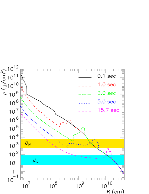
Figure 1: Shock and reverse-shock propagation in our numerical calculation. The density profile is shown at the indicated instances after core bounce. The density region $\rho_{\rm H}$ corresponds to resonant neutrino oscillations with the atmospheric mass difference, $\rho_{\rm L}$ to the solar one. The width of the bands reflects the expected energy range of SN neutrinos.

We here explore a new feature of the shock-wave “fingerprint” in the neutrino signal. Some time after the onset of the explosion a neutrino-driven baryonic wind develops and collides with the earlier, more slowly expanding supernova ejecta. A reverse shock is seen to form in all models which were computed with sufficient resolution and seems to be a generic feature, although the exact propagation history depends on the detailed dynamics during the early stages of the supernova explosion. Moreover, violent convective instabilities and large anisotropies are observed in the neutrino-heated layer behind the SN shock in multi-dimensional SN simulations and imply a significant angular variation of the instantaneous density profiles even in a single star. Still, the simultaneous propagation of a direct and an inverse shock wave imply that for some time the neutrinos may encounter two subsequent density discontinuities, leading to significantly different spectral features than are caused by a single crossing.

Numerical SN simulations do not yet lead to robust explosions so that it remains unclear if an important physical ingredient is missing in our understanding of the SN phenomenon. Even assuming that only minor aspects need to be tweaked, this situation implies that hydrodynamic state-of-the-art models of successful explosions with self-consistently determined neutrino fluxes and spectra do not exist at present. Therefore, we limit our discussion to a simple analytic study with a schematic density profile and an example of a detailed numerical model, using for both cases schematic primary neutrino fluxes and spectra that are representative for neutrino spectra discussed in the literature. In this way we identify a generic “double dip” feature caused by the presence of two density discontinuities. We find that the position of the two dips in time can be connected to the positions of the forward and reverse shock. The observation of the dips in different energy bins allows therefore not only the identification of the reverse shock but also to trace the propagation of both shocks. Since the neutrino conversion probabilities are energy dependent during the passage of the shocks through the H-resonance, neutrino oscillations can be detected even if the energy spectra of different neutrino flavors have the same shape but different luminosities.

We begin in Sec. 2 with an explanation of the reverse shock formation and a discussion of our numerical shock-propagation examples. In Sec. 3 we use a schematic model of the density profile to derive analytically the generic features imprinted on the observable neutrino signal. In Sec. 4 we use a concrete numerical example of shock and reverse shock propagation to calculate their typical signatures in a large $\bar{\nu}_{e}$ detector. In Sec. 5 we discuss and summarize our findings.

2 Our numerical SN model

Relying on the viability of the neutrino-heating mechanism we have performed simulations of supernova explosions that followed the evolution in spherical symmetry until more than 25 seconds after shock formation. In order to include the effects of convection we have also done runs in two dimensions for about one second of post bounce evolution. Because of the persistent problems of complete models in obtaining successful explosions (see, e.g., Ref. [3]), we replaced the high-density interior of the contracting nascent neutron star by a time-dependent inner boundary where the neutrino luminosities and spectra were imposed such that the neutrino energy transfer to the shock was sufficiently strong for shock revival (for more details, see Refs. [15, 16]).

The density profiles used for the evolving stellar background in the present work (cf. Fig. 1) were taken from simulations of a 15 $M_{\odot}$ progenitor [17]. Although the employed neutrino parameters are in the ballpark of results from elaborate neutrino transport calculations in supernovae, detailed information about neutrino fluxes and spectra that are consistent with explosion models and with the cooling history of the newly formed neutron star are currently not available. For this reason we consider the density profiles as exemplary for realistic supernova conditions and combine them with a schematic description of the neutrino emission that is supposed to contain generic features of the expected neutrino signal.

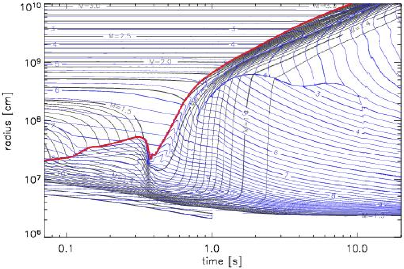
Figure 2: Early evolution (for times between 0.07 and 20 seconds after shock formation) of the supernova explosion (with an energy of about $1.5\times 10^{51}$ erg) of a 15 $M_{\odot}$ progenitor according to a spherically symmetric simulation in which the contracting neutron star was replaced by an inner boundary that acts as a neutrino source sufficiently intense to cause a neutrino-driven explosion. The black lines mark the space-time trajectories of selected mass shells, the blue lines represent corresponding contours of constant density, and the thick red line indicates the position of the supernova shock. The reverse shock and the contact discontinuity can be recognized from kinks and a compression of the isodensity curves in the region behind the forward shock.

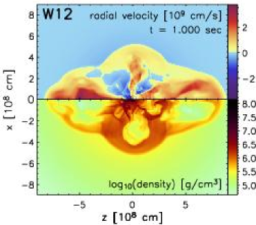
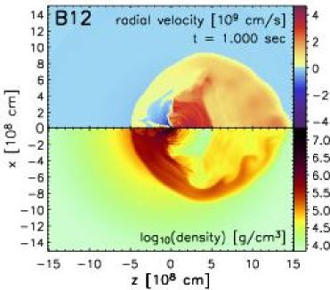
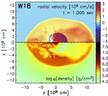
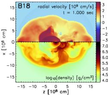
Figure 3: Radial velocity (upper half panels) and logarithm of density (lower half panels) color coded for four different two-dimensional simulations at one second after supernova shock formation. The explosion energies of these models are about $0.3\times 10^{51}$ erg, $0.4\times 10^{51}$ erg, $0.9\times 10^{51}$ erg, and $1.2\times 10^{51}$ erg (from top left to bottom right), respectively. The postshock structure is much more complex than in spherical symmetry, and depends strongly on the direction. While the contact discontinuity is distorted by hydrodynamic instabilities and marks the boundary between low-density neutrino-heated bubbles and matter that has been accreted and accelerated by the supernova shock, the reverse shock is a clear signature of the onset of a supersonically expanding neutrino-driven wind which runs into the earlier, slower supernova ejecta. But also multiple (reverse) shocks can occur due to collisions between downflows and neutrino-heated, expanding plasma.

The space-time evolution of the explosion of this 15 $M_{\odot}$ star in a spherically symmetric simulation (i.e., neglecting the effects of hydrodynamic instabilities) can be seen in Fig. 2. The shock expands from the point of its formation (not shown in this figure that displays only times later than 70 ms after core bounce) to a radius of about 100 km where it converts into a standing accretion shock. Its subsequent slow outward motion reflects the quasi-stationary adjustment of its position in response to the decreasing rate of mass infall from the outer stellar layers and to the energy deposition by neutrinos in the “gain region” behind the shock. At a radius of about 500 km the shock reaches a temporary maximum and starts retreating again because of decaying neutrino luminosities and a corresponding drop of the neutrino-heating rate. The subsequent sharp increase of the neutrino luminosities and of the energy deposition behind the shock is sufficient to trigger a successful explosion “in a second attempt.” This behavior is typical of one-dimensional simulations with conditions close to the threshold for shock revival.

On its way out the shock reverses the infall of the swept-up matter. Continuous neutrino energy transfer starts an outward acceleration of heated material in the gain layer around the neutron star. At the interface between this “neutrino-driven wind” to the outer ejecta a “contact discontinuity” is formed. It is visible as a strip of compressed density contours somewhat behind the outgoing supernova shock in Fig. 2. Even farther behind the forward shock, the neutrino-driven wind, whose velocity increases rapidly with distance from the neutron star, collides with more slowly moving material and is decelerated again. The strongly negative velocity gradient at this location steepens into a reverse shock when the wind velocity begins to exceed the local sound speed [18]. In the model of Fig. 2 this happens at $t\raise 1.29167pt\hbox{$\;>$\kern-7.5pt\raise-4.73611pt\hbox{$\sim\;$}}\,$800 ms post bounce at a radius $r\raise 1.29167pt\hbox{$\;>$\kern-7.5pt\raise-4.73611pt\hbox{$\sim\;$}}\,$1000 km.

The forward and reverse shocks are sharp discontinuities where density, pressure (as all other state variables) and velocity of the stellar plasma change on the microscopic (sub-millimeter) scale of the ion mean free path, on which the dissipation of kinetic to thermal energy in the shock occurs. In contrast, the “contact discontinuity” is characterized by a density jump but constant velocity and pressure. It emerges in the matter in the transition region between shock-accelerated and neutrino-heated supernova ejecta. Its width is therefore a result of the explosion dynamics and found to be 200–300 km in our one-dimensional model. However, because of our exponentially coarsening grid we are able to resolve this outward moving feature only for 2–3 seconds and are unable to make predictions of its exact structure at later times. A schematic representation of the described structure is given in Fig. 4.

The multi-dimensional situation is much more complex (cf. Fig. 3). The forward shock can now be highly deformed, and the reverse shock, which still separates the supersonically expanding neutrino-driven wind from subsonically moving outer ejecta, shows large angular variation. This reflects the anisotropy of the fluid flow between the shock and the neutron star, which is characterized by narrow downflows of cool gas and rising bubbles of low-density, neutrino-heated matter. These convective mass motions create a highly distorted structure in which multiple shocks can occur due to collisions of downflows with expanding, hot matter. Contact discontinuities follow the interface between the rising hot bubbles and shock accelerated plasma that has lower entropy and higher density. Their shape is affected by Rayleigh-Taylor and Kelvin-Helmholtz instabilities. Since the explosion is highly asymmetric, the exact structure varies strongly with the direction. Although the generic features of the one-dimensional situation are retained, the details of the multi-dimensional structure evolve chaotically from random initial perturbations and cannot be uniquely determined by models.

3 Effect of the shock waves on neutrino propagation

In present and planned water Cherenkov and scintillation detectors the main neutrino detection channel is the inverse beta decay reaction, $\bar{\nu}_{e}p\to ne^{+}$, that allows also for the reconstruction of the neutrino energies. Therefore we consider only the $\bar{\nu}_{e}$ spectrum in the following. However an analogous analysis can be easily performed in the neutrino channel for a detector able to measure the ${\nu_{e}}$ spectrum, using e.g. liquid argon.

The antineutrino spectra arriving at the Earth are determined by the primary antineutrino spectra as well as the neutrino mixing scenario,

$$F_{\bar{\nu}_{e}}(E)=\bar{p}(E)F_{\bar{\nu}_{e}}^{0}(E)+[1-\bar{p}(E)]F_{\bar{\nu}_{x}}^{0}(E)\,,$$ (1)

where $\bar{p}(E)$ is the survival probability of a $\bar{\nu}_{e}$ with energy $E$ after propagation through the SN mantle, the superscript zero denotes the primary fluxes, and ${\bar{\nu}_{x}}$ stands for either ${\bar{\nu}}_{\mu}$ or ${\bar{\nu}}_{\tau}$. In general, all quantities of Eq. (1) are not only energy but also time dependent. In particular the survival probability $\bar{p}(E)$ becomes time dependent during the passage of the shocks through the H-resonance. Before we discuss the effect of the shock propagation on the neutrino spectra, we first recall the case of three-flavor neutrino oscillations in a static density profile. In this case, $\bar{p}(E)$ is not only constant in time, but also independent of energy if $\sin^{2}\vartheta_{13}\raise 1.29167pt\hbox{$\;<$\kern-7.5pt\raise-4.73611pt\hbox{$\sim\;$}}10^{-5}$ or $\sin^{2}\vartheta_{13}\raise 1.29167pt\hbox{$\;>$\kern-7.5pt\raise-4.73611pt\hbox{$\sim\;$}}10^{-3}$. Since about 60% of the observed neutrinos will be detected in the first two seconds after bounce, i.e. before the shock reaches the H-resonance of low-energy neutrinos, it is for many purposes sufficient to perform the simpler analysis of neutrino propagation through the static envelope of the progenitor. For us, the static case discussed in the next subsection serves as a reference to measure the modulations induced by the propagating shock.

3.1 Static case before the arrival of the shock wave at the H-resonance

The survival probability is determined by the flavor conversions that take place in the resonance layers, where $\rho_{\rm res}\approx m_{\rm N}\Delta m^{2}_{i}\cos 2\vartheta/(2\sqrt{2}G_{\rm F}Y_{\rm e}E)$. Here $\Delta m^{2}_{i}$ and $\vartheta$ are the relevant mass difference and mixing angle of the neutrinos, $m_{\rm N}$ is the nucleon mass, $G_{\rm F}$ the Fermi constant and $Y_{\rm e}$ the electron fraction. In contrast to the solar case, SN neutrinos must pass through two resonance layers: the H-resonance layer at $\rho_{\rm H}\sim 10^{3}$ g/cm³ corresponds to $\Delta m^{2}_{\rm atm}$, whereas the L-resonance layer at $\rho_{\rm L}\sim 10$ g/cm³ corresponds to $\Delta m^{2}_{\odot}$. This hierarchy of the resonance densities, along with their relatively small widths, allows the transitions in the two resonance layers to be considered independently [10].

The neutrino survival probabilities can be characterized by the degree of adiabaticity of the resonances traversed, which are directly connected to the neutrino mixing scheme. In particular, whereas the L-resonance is always adiabatic and appears only in the neutrino channel, the adiabaticity of the H-resonance depends on the value of $\vartheta_{13}$, and the resonance shows up in the neutrino or antineutrino channel for a normal or inverted mass hierarchy respectively. Table 1 shows the survival probabilities for neutrinos, $p$, and antineutrinos, $\bar{p}$, in various mixing scenarios. For intermediate values of $\vartheta_{13}$, i.e. $10^{-5}\raise 1.29167pt\hbox{$\;<$\kern-7.5pt\raise-4.73611pt\hbox{$\sim\;$}}\sin^{2}\vartheta_{13}\raise 1.29167pt\hbox{$\;<$\kern-7.5pt\raise-4.73611pt\hbox{$\sim\;$}}10^{-3}$, the survival probabilities depend even without shock on energy as well as the details of the density profile of the SN.

For large values of $\vartheta_{13}$ and the static density profile of the progenitor, the H-resonance is adiabatic. In the case of normal mass hierarchy, scenario A, the resonance takes place in the neutrino channel, and antineutrinos are not affected. For an inverted mass hierarchy, scenario B, the resonance occurs in the antineutrino channel, so that practically all the primary ${\bar{\nu}_{e}}$ are converted to $\bar{\nu}_{3}$ and arrive at the Earth as ${\bar{\nu}_{x}}$. This corresponds to an almost complete interchange of ${\bar{\nu}_{e}}$ and ${\bar{\nu}_{x}}$ spectra. In scenario C, the resonance is strongly non-adiabatic, and hence ineffective. In both the scenarios A and C, the primary ${\bar{\nu}_{e}}$ leave the star as $\bar{\nu}_{1}$, which implies a partial mixing between ${\bar{\nu}_{e}}$ and ${\bar{\nu}_{x}}$ spectra.

Scenario	Hierarchy	$\sin^{2}\vartheta_{13}$	$p$	$\bar{p}$
A	Normal	$\raise 1.29167pt\hbox{$\;>$\kern-7.5pt\raise-4.73611pt\hbox{$\sim\;$}}10^{-3}$	0	$\cos^{2}\vartheta_{\odot}$
B	Inverted	$\raise 1.29167pt\hbox{$\;>$\kern-7.5pt\raise-4.73611pt\hbox{$\sim\;$}}10^{-3}$	$\sin^{2}\vartheta_{\odot}$	0
C	Any	$\raise 1.29167pt\hbox{$\;<$\kern-7.5pt\raise-4.73611pt\hbox{$\sim\;$}}10^{-5}$	$\sin^{2}\vartheta_{\odot}$	$\cos^{2}\vartheta_{\odot}$

Table 1: Survival probabilities for neutrinos, $p$, and antineutrinos, $\bar{p}$, in various mixing scenarios for a static density profile.

3.2 Shock waves passing through the H-resonance

In our numerical model, the outgoing shock wave reaches the H-resonance layer around two seconds after bounce and the L-resonance layer around ten seconds after bounce. Since for $t\raise 1.29167pt\hbox{$\;>$\kern-7.5pt\raise-4.73611pt\hbox{$\sim\;$}}11$ s the H-resonance is adiabatic, neutrinos created as $\bar{\nu}_{e}$ arrive in case B as $\bar{\nu}_{3}$ at the L-resonance. Thus, the L-resonance that mixes 12-states does not affect the survival probability $\bar{p}$, independent of the passage of shock waves. In contrast, it depends on the neutrino mixing scenario, whether the shock waves modulate the neutrino spectra during their passage through the H-resonance: The cases A and C will not show any evidence of shock wave propagation in the observed ${\bar{\nu}_{e}}$ spectrum, either because there is no resonance in the antineutrino channel as in scenario A, or because the resonance is always strongly non-adiabatic as in scenario C. However, in scenario B, the sudden change in the density breaks the adiabaticity of the resonance, leading to observable consequences in the ${\bar{\nu}_{e}}$ spectrum. Let us discuss this scenario henceforth.

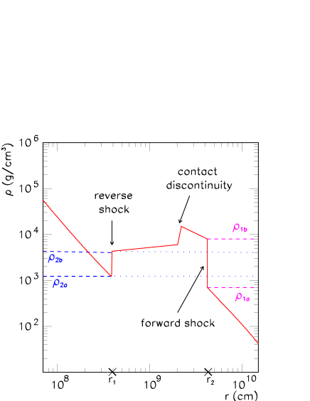
Figure 4: Schematic density profile in the presence of a forward and reverse shock wave. Between forward and reverse shock a contact discontinuity can appear.

In order to analytically understand the signatures of the shock wave in the observed ${\bar{\nu}_{e}}$ spectrum, let us first assume that the shock wave causes the adiabatic H-resonance to become completely non-adiabatic at the forward shock front and the reverse shock front, while at all other places the resonance remains adiabatic. In the snapshot of the shock wave shown in Fig. 4, non-adiabatic transitions take place only at the two radii $r_{1}$ and $r_{2}$, where the forward and the reverse shock waves are present at that time.

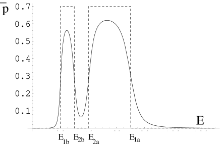
Figure 5: Survival probability $\bar{p}$ as a function of energy $E$ assuming $|\vartheta_{a}-\vartheta_{b}|\approx\pi/2$ (dotted line) or using Eq. (3) (solid line) with $\cos^{2}\vartheta_{\odot}=0.7$.

Neutrinos with energy $E$ undergo H-resonance in the region of density

$$\rho=\frac{m_{\rm N}\Delta m^{2}_{\rm atm}\cos 2\vartheta_{13}}{2\sqrt{2}G_{\rm F}Y_{\rm e}E}\approx 600\,{\rm g/cm}^{3}\;\cos 2\vartheta_{13}\>\frac{25~{}{\rm MeV}}{E}\>\frac{1}{Y_{\rm e}}\,.$$ (2)

The maximum and minimum densities at the two shock fronts, as illustrated in Fig. 4, then directly give the range of energies that undergo a non-adiabatic resonance at these shock fronts. We introduce now the two approximations of our toy-model used in this subsection: First, we assume that all resonances are either completely adiabatic or completely non-adiabatic. Second, we require that the density jump at the resonances is large, i.e. that the change of the medium mixing angle is close to $\pi/2$. Then the survival probability $\bar{p}(E)$ is a rectangular wave as a function of energy, as shown in Fig. 5 with a dotted line. Clearly, as the shock wave propagates to lower densities, the “turning points” of the square wave shift upwards in energy. The amplitude of the square wave, $\cos^{2}\vartheta_{\odot}$, is fixed by the value of the solar mixing angle. We can relax the second approximation and use the result that, if the density changes sharply from $\rho_{b}$ to $\rho_{a}$, the survival probability for ${\bar{\nu}_{e}}$ is

$$\bar{p}=\sin^{2}(\vartheta_{a}-\vartheta_{b})\cos^{2}\vartheta_{\odot}\,,$$ (3)

where $\vartheta_{a}$ and $\vartheta_{b}$ are the values of $\vartheta_{13}$ in matter at the densities $\rho_{a}$ and $\rho_{b}$, respectively. Using this, the rectangular wave for $\bar{p}$ gets modified as shown in Fig. 5 with a solid line. However, in order to get a simple understanding of the new features of the conversion probability we will use the rectangular wave for $\bar{p}$ in the rest of this section.

The primary spectra of neutrinos can be parameterized by [19, 20]

$$F^{0}_{i}(E)=\frac{\Phi_{i}}{\langle E_{i}\rangle}\,\frac{\beta_{i}^{\beta_{i}}}{\Gamma(\beta_{i})}\left(\frac{E}{\langle E_{i}\rangle}\right)^{\beta_{i}-1}\exp\left(-\beta_{i}\frac{E}{\langle E_{i}\rangle}\right)\,,$$ (4)

where $\langle E_{i}\rangle$ denotes their average energy, $\beta_{i}$ is a dimensionless parameter that relates to the width of the spectrum and typically takes on values 3.5–6, depending on the flavor and the phase of neutrino emission. Let us approximate the energy dependence of the cross section of the inverse beta decay reaction by $E^{2}$, and assume an ideal detector. Using Eq. (1), Table 1 and the survival probability as shown in Fig. 5, the number of ${\bar{\nu}_{e}}$ events observed in a certain time interval is

$$N_{\rm obs}={\cal N}\left[\Phi_{\bar{\nu}_{x}}\frac{\langle E_{\bar{\nu}_{x}}\rangle^{2}}{\beta_{\bar{\nu}_{x}}^{2}}\frac{\Gamma(\beta_{\bar{\nu}_{x}}+2)}{\Gamma(\beta_{\bar{\nu}_{x}})}+\cos^{2}\vartheta_{\odot}(\Phi_{\bar{\nu}_{e}}g_{2}^{\bar{\nu}_{e}}-\Phi_{\bar{\nu}_{x}}g_{2}^{\bar{\nu}_{x}})\right]\,,$$ (5)

where ${\cal N}$ is a normalization constant, $\Gamma(z)$ is the Euler gamma function, and we have introduced the functions

$$g_{k}^{i}=\frac{\langle E_{\bar{\nu}_{x}}\rangle^{k}}{\beta_{i}^{k}\Gamma(\beta_{i})}\left[\Gamma\left(a,\frac{E_{1}}{\langle E_{i}\rangle}\beta_{i},\frac{E_{2}}{\langle E_{i}\rangle}\beta_{i}\right)+\Gamma\left(a,\frac{E_{3}}{\langle E_{i}\rangle}\beta_{i},\frac{E_{4}}{\langle E_{i}\rangle}\beta_{i}\right)\right]\,.$$ (6)

Here, $\Gamma(a,b,c)=\int_{b}^{c}dt\>t^{a-1}e^{-t}$ is a generalized incomplete Gamma function, and $a=\beta+k$. The values $E_{1},E_{2},E_{3},E_{4}$ are the same as $E_{1a},E_{1b},E_{2a},E_{2b}$ in ascending order. The $m$th moment of the total energy $E_{\rm obs}^{m}$ deposited in the detector during a certain time interval is similarly given by

$$\hskip-28.45274ptE_{\rm obs}^{m}={\cal N}\left[\Phi_{\bar{\nu}_{x}}\frac{\langle E_{\bar{\nu}_{x}}\rangle^{2+m}}{\beta_{\bar{\nu}_{x}}^{2+m}}\frac{\Gamma(\beta_{\bar{\nu}_{x}}+2+m)}{\Gamma(\beta_{\bar{\nu}_{x}})}+\cos^{2}\vartheta_{\odot}(\Phi_{\bar{\nu}_{e}}g_{2+m}^{\bar{\nu}_{e}}-\Phi_{\bar{\nu}_{x}}g_{2+m}^{\bar{\nu}_{x}})\right]\,.$$ (7)

Since the values of $E_{1a}$, $E_{1b}$, $E_{2a}$, $E_{2b}$ change as a function of time, so do the values of $N_{\rm obs},E_{\rm obs}$. As time goes on, the shock wave reaches layers with smaller densities and therefore, according to Eq. (2), higher-energetic neutrinos are affected by the wave propagation. The time dependence of the numerical profiles can be imitated starting from $t=1\,$s by $E_{i}(t)=(t/{\rm s})^{a_{i}}\ln(t/{\rm s})$ MeV, and where $a_{i}=\{1.3,1.5,1.7,2.0\}$. As a consequence, the double square structure in the survival probability shown in Fig. 5 keeps on shifting towards higher energies with time.

In order to study the model dependence of our results, we consider three models that give very different predictions for the neutrino spectra. Two of them, G1 and G2, are motivated by the recent Garching calculation [21] that includes all relevant neutrino interaction effects like nucleon bremsstrahlung, neutrino pair processes, weak magnetism, nucleon recoils and nuclear correlation effects. The third one is from the Livermore simulation [22] that represents more traditional predictions for flavor-dependent SN neutrino spectra used in many previous analyses. The parameters of these models are shown in Table 2.

• Model	$\langle E_{0}(\nu_{e})\rangle$	$\langle E_{0}({\bar{\nu}_{e}})\rangle$	$\langle E_{0}({\nu_{x}})\rangle$	$\frac{\Phi_{0}(\nu_{e})}{\Phi_{0}(\nu_{x})}$	$\frac{\Phi_{0}({\bar{\nu}_{e}})}{\Phi_{0}(\nu_{x})}$
  L	12	15	24	2.0	1.6
  G1	12	15	18	0.8	0.8
  G2	12	15	15	0.5	0.5

Table 2: The parameters of the used primary neutrino spectra models motivated from SN simulations of the Garching (G1, G2) and the Livermore (L) group. We assume $\beta_{\bar{\nu}_{x}}=4$ and $\beta_{\bar{\nu}_{e}}=5$.

In Fig. 6, we show the values of the average event energy $\langle E_{e}\rangle\equiv E_{\rm obs}/N_{\rm obs}$ observed (left) as well as $\xi\equiv\langle E_{e}^{2}\rangle/\langle E_{e}\rangle^{2}$ (right) as functions of time for the three models of Tab 2. The parameter $\xi$ measures the pinching of the observed spectrum and indicates therefore if it is a superposition of primary spectra with different shapes. We compare the case where both forward and reverse shock waves are present with the forward shock only case. We approximate the latter by setting $E_{2a}=E_{2b}$.

In the absence of shock waves, the adiabaticity of the propagation in case B ensures that the ${\bar{\nu}_{e}}$ flux arriving at the Earth, $F_{\bar{\nu}_{e}}(E)$, basically coincides with $F^{0}_{\bar{\nu}_{x}}(E)$. Thus, breaking that adiabaticity will imply a partial presence of $F^{0}_{\bar{\nu}_{e}}(E)$ in $F_{\bar{\nu}_{e}}(E)$. Therefore any departure of the observables from their values in the no-shock case induced by the shock depends strongly on which part of the energy spectra is affected by the shock wave, and how different the original spectra are at those energies.

At early times, $t\raise 1.29167pt\hbox{$\;<$\kern-7.5pt\raise-4.73611pt\hbox{$\sim\;$}}4$ s, the shock affects only the low-energy part of the spectra, $E\raise 1.29167pt\hbox{$\;<$\kern-7.5pt\raise-4.73611pt\hbox{$\sim\;$}}20$ MeV. At these energies, the ratio $F^{0}_{\bar{\nu}_{x}}(E)/F^{0}_{\bar{\nu}_{e}}(E)$ varies for different SN models: it is smaller than one in model L and larger than one in models G1 and G2. Therefore, any modulation in the observables at these early times will strongly depend on the model considered. At later times, $t>4$ s, neutrinos with higher energies, $E\raise 1.29167pt\hbox{$\;>$\kern-7.5pt\raise-4.73611pt\hbox{$\sim\;$}}20$ MeV, feel the breakdown of the adiabaticity. At these energies, the ${\bar{\nu}_{x}}$ flux is in all models larger than the ${\bar{\nu}_{e}}$ flux, $F^{0}_{\bar{\nu}_{x}}(E)>F^{0}_{\bar{\nu}_{e}}(E)$. Therefore our prediction for the observable modulation of SN neutrino spectra at later times, $t\raise 1.29167pt\hbox{$\;>$\kern-7.5pt\raise-4.73611pt\hbox{$\sim\;$}}4$ s, will be model independent and thus more robust. For this reason, we will basically concentrate the discussion on the modulation of the observables arising at these times.

The main effect visible in the time evolution of $\langle E_{e}\rangle$ shown in the left panel of Fig. 6 is a decrease of $\langle E_{e}\rangle$ when the shock passes the resonance region and reduces the number of events at high energies. However, the details will depend on the features of the shock propagation. If only the forward shock wave is present, a deep and wide dip is expected. If moreover a reverse shock is formed, a double dip will be observed: the positions of the two dips correspond to the times when one of the peaks in the survival probability in Fig. 5 coincides with the peak energy of the antineutrino spectrum. In the case of $\xi=\langle E_{e}^{2}\rangle/\langle E_{e}\rangle^{2}$ the double dip structure becomes a double bump. In contrast to an energy-independent survival probability, $\xi$ is not always increased by mixing but can be also reduced.

It is remarkable that even in the model G2, where the original mean energies $\langle E_{i}\rangle$ are exactly the same, the energy dependence of the conversion probability results in an observable effect of the shock wave propagation, because of the flavor-dependent fluxes.

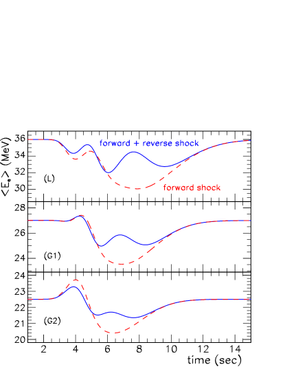
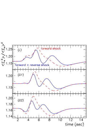
Figure 6: Time dependences of the observables $\langle E_{e}\rangle$ (left) and $\langle E_{e}^{2}\rangle/\langle E_{e}\rangle^{2}$ (right) for different primary spectra, (L, G1, G2), and assuming both forward and reverse shock (blue solid line) and only forward shock wave (red dashed line).

Note that in this section we have assumed that the level crossings are completely adiabatic except at the forward and reverse shocks. For $\sin^{2}\vartheta_{13}$ close to its current upper limit, this is very likely to be the case. In the next section, we numerically calculate the survival probability without the foregoing assumption, and find that the qualitative features obtained here do indeed survive in the complete numerical calculation. These features are thus robust, and though illustrated here for the case of a special shock profile, should be valid for a general case.

4 Detection of the shock and the reverse shock

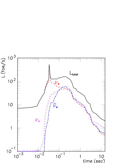
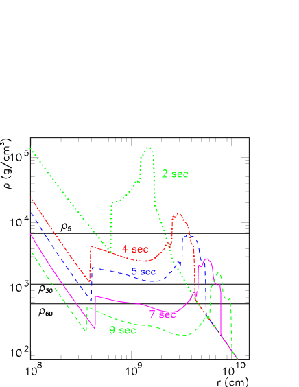
Figure 7: Left: Time dependence of the neutrino luminosities $L$ used, from Ref. [22]. Right: Density profiles at different times obtained from the numerical simulations of section 2. The H-resonance density, $\rho_{\rm H}$, for different neutrino energies, 5, 30 and 60 MeV, is also shown.

In this section, we examine in more detail the signatures of the forward and reverse shock propagation imprinted on the neutrino signal of a future galactic SN. The different ingredients used for the simulation are

• Initial fluxes: we assume for the time dependence of the total luminosity the one given in Ref. [22], shown in the left panel of Fig. 7. We use the parameterization of Eq. (4) for the spectral shape, with the values given in Tab. 2.

• The density profile of the SN envelope at different times as discussed in Sec. 2. In the right panel of Fig. 7, we show the effect of the forward and the reverse-shock wave on the density profiles at several instances. The basic structures of the numerical profiles coincide well with the schematic profiles from Fig. 4 used in our analytical discussion, except at early times, where $\rho_{2a}\raise 1.29167pt\hbox{$\;<$\kern-7.5pt\raise-4.73611pt\hbox{$\sim\;$}}\rho_{1a}$.

• The numerically calculated survival probability $\bar{p}(E,t)$.

• Detector: we simulate the neutrino signal at a megaton water Cherenkov detector assuming a SN distance of 10 kpc. The detector response is taken care of in the manner described in Ref. [23]. The neutrino signal is dominated by the inverse beta reaction ${\bar{\nu}_{e}}p\to ne^{+}$, while all other reactions have a negligible influence on the analysis below. In future, the addition of Gd may allow for the efficient tagging of this reaction [24]. Therefore, we take into account only the inverse beta reactions in the following analysis.

• Neutrino mixing parameters: we concentrate on case B, i.e. an inverted mass hierarchy and large $\vartheta_{13}$. In particular, we use the following numerical values for the relevant parameters, $\Delta m^{2}_{\odot}=6.9\times 10^{-5}$ eV², $\tan^{2}\vartheta_{\odot}=0.42$, $\Delta m^{2}_{\rm atm}=2.6\times 10^{-3}$ eV², and $\tan^{2}\vartheta_{13}=10^{-2}$. However, we have checked that the signatures of the shock propagation like the “double-dip” feature are detectable even for $\tan^{2}\vartheta_{13}=5\times 10^{-5}$.

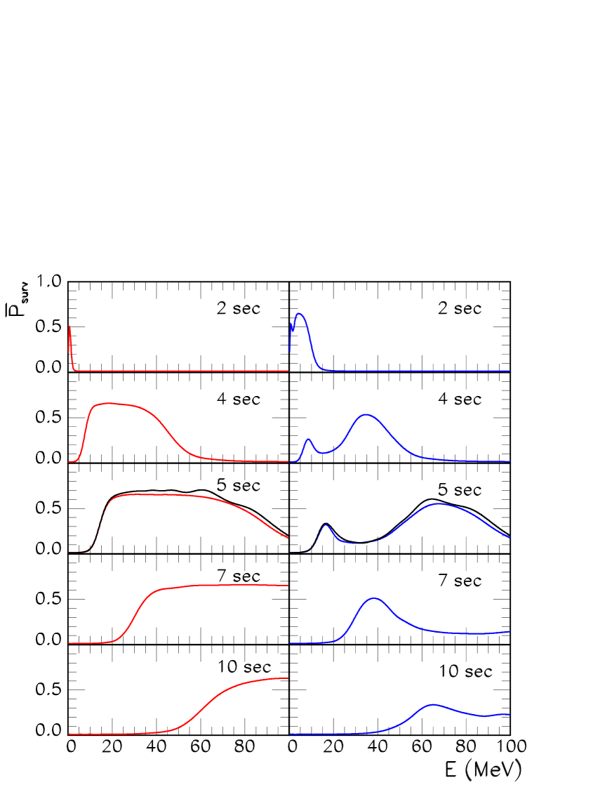
Figure 8: Survival probability $\bar{p}(E,t)$ as function of energy at different times averaging in energies with the energy resolution of Super-Kamiokande; for a profile with only a forward shock (left) and a profile with forward and reverse shock (right). At $t=5$ s, we show $\bar{p}(E,t)$ including Earth matter effects for a zenith angle of the SN of $62^{\circ}$ (black line).

The key ingredient to observe signatures of the shock wave propagation is the time and energy dependence of the neutrino survival probability. In Fig. 8, we show the energy dependence of $\bar{p}(E,t)$ averaged with the energy resolution function of Super-Kamiokande, for the case with (right panel) and without (left panel) a reverse shock. To simulate the latter case, we removed by hand the reverse shock from the numerical density profiles.

Qualitatively, we observe the same features as using the analytical approximation of Sec. 3: While the survival probability has a single peak if there is only a forward shock propagating, the reverse shock superimposes a dip at those energies for which the resonance region is passed by both shock waves. All these structures move in time towards higher energies, as the shock waves reach regions with lower density. The width and location of the peaks depend on the particular values of $E_{1a},E_{1b},E_{2a},E_{2b}$ at each instant. We can observe, for example, that at $t=2$ s only low energy neutrinos, $E\sim 10$ MeV, are affected by the reverse shock. A little bit later, at $t=5$ s, neutrinos with energies $E\sim 10$–15 MeV are influenced by the forward shock wave (the first peak), while those with $E\sim 20$–60 MeV feel the effect of both the reverse and the forward shocks. The effect of the two strongly non-adiabatic transitions cancel partially and $\bar{p}(E,t)$ has a valley around $\sim 30$ MeV. For $E\raise 1.29167pt\hbox{$\;>$\kern-7.5pt\raise-4.73611pt\hbox{$\sim\;$}}60$ MeV, neutrinos cross only one shock wave, thus a second peak appears in $\bar{p}(E,t)$. At later times, this pattern is basically repeated, only shifted to higher and higher energies.

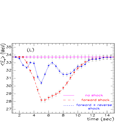
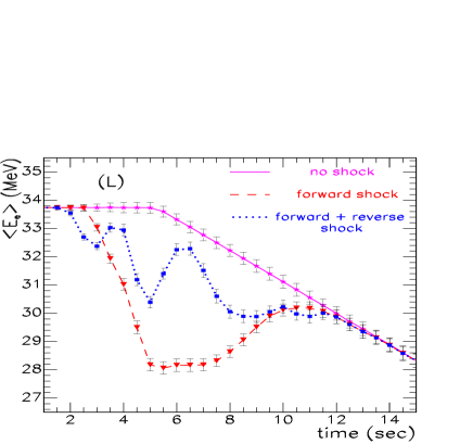
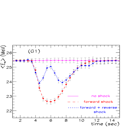
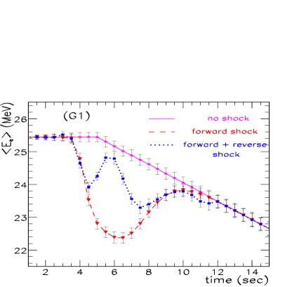
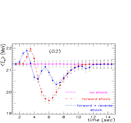
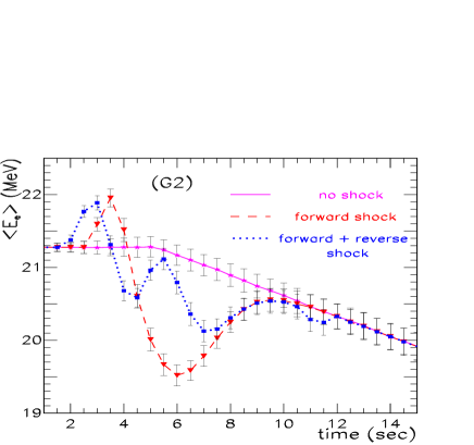
Figure 9: The average energy of $\bar{\nu}p\to ne^{+}$ events binned in time for a static density profile (magenta), a profile with only a forward shock (red) and with forward and reverse shock (blue). In the left panels we use $\langle E_{i}\rangle={\rm const.}$, whereas in the right panels $\langle E_{i}\rangle$ decreases for $t>5$ s. The error bars represent 1 $\sigma$ errors in any bin.

The first observable we consider is the average of the measured positron energies, $\langle E_{e}\rangle$, with a time binning of 0.5 s. In Fig. 9, we show $\langle E_{e}\rangle$ for various cases together with the one sigma errors: Each of the six panels contains the case that no shock wave influences the neutrino propagation, the case of only a forward shock wave and of both forward and reverse shock wave. In the three left panels the $\langle E_{i}\rangle$ are constant in time, while in the three right panels we assume that the $\langle E_{i}\rangle$ decrease linearly after 5 s. Finally, the upper, middle and lower panels show the three models L, G1 and G2 for the primary neutrino spectra given in Table 2.

As our most important result we find that the effects of the shock wave propagation are clearly visible in the neutrino signal of a megaton detector, independent of the assumptions about the initial neutrino spectra. Moreover, it is not only possible to detect the shock wave propagation in general, but also to identify the specific imprints of the forward and reverse shock versus the forward shock only case. The signature of the reverse shock is its double-dip structure compared to the one-dip of a forward shock only, as predicted by our analytical model in Fig. 6. While the presence or absence of structures at early times does depend on the initial fluxes and the details of the density profiles, the two-dip pattern is a robust signature of the presence of a reverse shock. To study the dependence of the double-dip structure on the value of $\vartheta_{13}$, we show $\langle E_{e}\rangle$ as function of time for different 13-mixing angles in the left panel of Fig. 10. Even for as small values as $\tan^{2}\vartheta_{13}=5\times 10^{-5}$ the double-dip is still clearly visible, while for $\tan^{2}\vartheta_{13}=1\times 10^{-5}$ only a bump modulates the neutrino signal.

Next we discuss the possibility to detect the imprint of the shock waves in other observables. To shorten the exposition, we consider only one model (L) together with a linear decrease of $\langle E_{i}\rangle$ after $t=5$ s. In Fig. 10, we show the time dependence of the observable $\xi=\langle E_{e}^{2}\rangle/\langle E_{e}\rangle^{2}$. If the shock does not influence the neutrino spectra, i.e. $\bar{p}\approx 0$, then $\xi=\xi_{0}=(\beta_{\bar{\nu}_{x}}+3)/(\beta_{\bar{\nu}_{x}}+2)$. For a mixed spectrum, with $\bar{p}(E)$ independent of energy, we have $\xi>\xi_{0}$ in general. However, for a strongly energy dependent $\bar{p}(E)$ as in the case of a shock, $\xi$ can increase or decrease depending on the details of $\bar{p}(E)$ and the primary spectra. Such modulations in the value of $\xi$ that coincide in time with the modulations in $\langle E_{e}\rangle$ act as a confirming evidence for the passage of the shock wave.

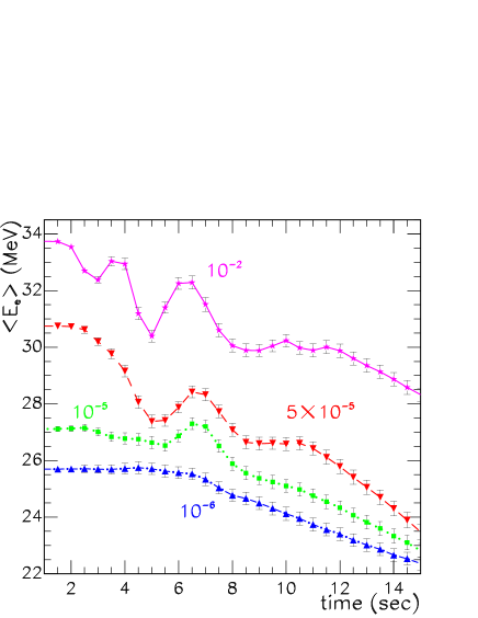
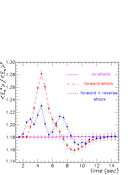
Figure 10: Left: Time dependence of $\langle E_{e}\rangle$ for a profile with a forward and reverse shock for several values of $\tan^{2}\vartheta_{13}$ as indicated; for model L. Right: Time dependences of the observable $\xi=\langle E_{e}^{2}\rangle/\langle E_{e}\rangle^{2}$ for a static density profile (magenta), a profile with only a forward shock (red) and with forward and reverse shock (blue).

Another observable that can be exploited is the total number of detected events. In the left panel of Fig. 11, we show the number of events binned in time. This observable is particularly interesting for detectors like IceCube with poor or no energy resolution at all for SN neutrinos. If the luminosities are fast decreasing with time, the modulations introduced by the time-behavior of $\bar{p}(E,t)$ may be difficult to disentangle from the overall time-behavior of the luminosities. Nevertheless, even a detector without energy resolution like IceCube has a potential to discover the imprint of propagating shock waves on the neutrino signal, if the luminosities are not decreasing as fast as found in Ref. [22].

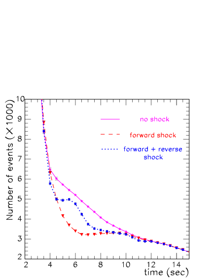
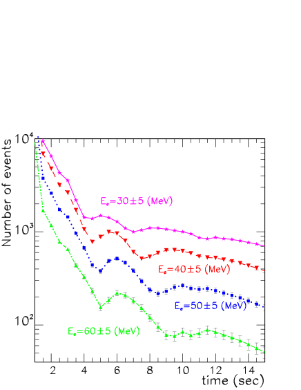
Figure 11: Left: Total number of events detected as function of time. Right: Number of events binned per energy decade as function of time for forward and reverse shock.

Since the information about the shock fronts is encoded in the energy and time dependence of the survival probability $\bar{p}(E,t)$, one can expect that the number of events in a fixed energy range is a more useful observable than the total number of events. In the right panel of Fig. 11, we show therefore the number of events binned in energy intervals of 10 MeV as function of time for the case of a reverse shock. We can observe clearly how the positions of the two dips change in each energy bin. It is remarkable that the double-dip feature is not only stronger after binning, but also allows one to trace the shock propagation: Given the neutrino mixing scheme, the neutrino energy fixes the resonance density. Therefore, the progress of the shock fronts can be read off from the position of the double-dip in the neutrino spectra of different energy.

We illustrate this by examining the time evolution of the number of events in the bin $40\pm 5$ MeV in detail. From Fig. 12, right panel, it can be read off that between 4.5–7.5 s, the neutrinos with this energy pass through two nonadiabatic resonances, i.e. both the forward and the reverse shock are present in the regions with density $\rho_{40}\approx 850$ g/cm³. Between 7.5 s and 9.5 s, only one of the shock fronts is present at this density. This inferred behavior of the shock wave can be seen to correspond with the shock profile used, see the left panel of Fig. 12. For times before 4.5 s and after 9.5 s, the data is not able to say anything concrete about the shock wave propagation.

If only the forward shock is present, then Fig. 12 still allows us to infer that one shock wave was present in the region $\rho_{40}$ between 5–9.5 s. No concrete conclusions can be drawn about the behavior of the shock wave beyond this time interval.

The number of shock waves present in a region with any given density $\sim 10^{3}$ g/cm³ can similarly be extracted from the data by considering the time evolution of the number of events in the energy bin corresponding to that density. An extrapolation would allow one to trace the positions of the forward and the reverse shock waves for times between 1–10 s.

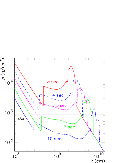
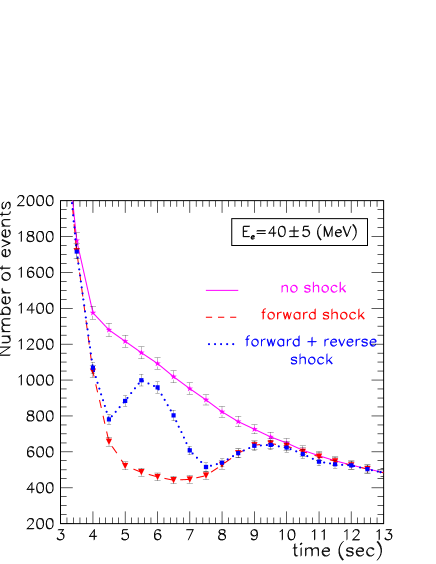
Figure 12: Left: Density profiles at different times with the resonance layer of neutrino with $E=40$ MeV superimposed. Right: Number of events expected in the energy range $E=40\pm 5$ MeV as function of time.

Until now we have neglected the possibility that other discontinuities in addition to the forward and reverse shock can influence the neutrino propagation. However, because of the decreasing resolution in our simulation at large radii as described in Sec. 2, we are only able to resolve the outward moving contact discontinuity for 2–3 seconds. Its width at that time is found to be 200–300 km in our one-dimensional model. Hydrodynamic instabilities are expected to widen the contact discontinuity, and we expect therefore that the neutrino evolution is adiabatic also at later times at this discontinuity. But to get an idea of the possible influence of this discontinuity on observables, we have steepened it by hand for $t>3$ s, so that the neutrino evolution becomes strongly non-adiabatic at this point. In Fig. 13, we show the detected $\langle E_{e}\rangle$ in this case. Since now there are three shocks (and six associated energies), the structures in $\langle E_{e}\rangle$ become more complicated but the imprint of the shock wave is still clearly visible. In particular, there are effects of the shock wave propagation at later times than in the previous cases, because for the density profiles considered in our study the largest density affected by this new discontinuity is larger than the maximum of $\rho_{1a}$ and $\rho_{1b}$.

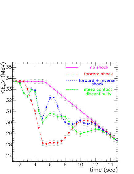
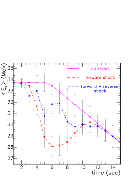
Figure 13: Left: Observed $\langle E_{e}\rangle$ for a static density profile (magenta), a profile with only a forward shock (red), with forward and reverse shock (blue), and in the case that the contact discontinuity is steepened by hand (green). Right: Observed $\langle E_{e}\rangle$ in Super-Kamiokande, color code as in the left panel.

Finally, we want to discuss if the largest currently operating detector, Super-Kamiokande, can observe the signatures of shock wave propagation. Compared to a megaton detector, the event rate in Super-Kamiokande is reduced by a factor of 30. Therefore, we plot in the right panel of Fig. 13 the mean event energy $\langle E_{e}\rangle$ with one second time bins in order to decrease the statistical error. The features of the different shock propagation scenarios remain visible, but are now more difficult to disentangle because of the larger errors. However, one should keep in mind that the number of events is not only related to the volume of the detector but also to the distance to the SN. Thus, the potential of Super-Kamiokande to yield important clues about the shock propagation cannot be dismissed.

5 Summary

We have performed simulations of supernova explosions adjusting the neutrino energy transfer to the shock so that a successful explosion resulted. Following the time evolution in spherical symmetry until more than 25 seconds after shock formation, we have found that in addition to the forward shock wave a reverse shock forms when the supersonically expanding neutrino-driven wind collides with the slower earlier SN ejecta. Both the forward and reverse shock are sharp discontinuities where the density changes on a sub-millimeter scale.

The sudden density jump at the two shock fronts results in a strongly non-adiabatic evolution of neutrino flavor oscillations, when the shocks cross the H-resonance layer. For a “large” 13-mixing angle, $\sin^{2}\vartheta_{13}\gg 10^{-5}$, the MSW enhancement of flavor conversion that is otherwise working is interrupted during the shock passage. This break-down of adiabaticity results in a reduction of the average energy and number of detected $\bar{\nu}_{e}$ events for an inverse neutrino mass hierarchy (case B) or of $\nu_{e}$ events for a normal hierarchy (case A). The reduced event rate during the shock passage through the H-resonance allows even experiments with missing energy resolution for SN neutrinos, as e.g. IceCube, to observe effects of the shock propagation.

The characteristic signature for the presence of two shocks is the “double-dip” feature in the time-binned energy spectrum of observed electron-neutrino events. We have found that already Super-Kamiokande can potentially distinguish between different shock propagation scenarios, while a megaton detector may be able to trace the time-evolution of forward and reverse shocks.

The modulation of SN neutrino spectra by propagating shocks is only possible if $\vartheta_{13}$ is “large,” $\sin^{2}\vartheta_{13}\gg 10^{-5}$. Observing these features in the neutrino signal of a future galactic SN would therefore indicate that the measurement of $\vartheta_{13}$ and the detection of leptonic CP violation may be within reach. In addition, the detection of any modulation in the $\bar{\nu}_{e}$ or the $\nu_{e}$ spectrum by shock effects would identify the neutrino mass hierarchy. Remarkably, observing features of SN shock propagation is complementary to the detection of Earth matter effects: while observing modulations by SN shocks in the $\bar{\nu}_{e}$ spectrum identifies case B, modulations by Earth matter effects exclude this case.

We want to close with a speculative remark about the time-structure of the neutrino events from SN 1987A. The events observed by the Kamioka experiment can be grouped into two time bins: nine events during the first two seconds, then three more events after a time gap of six seconds. Intriguingly, such a time structure is compatible with the modulation of the neutrino signal by SN shocks, if the neutrino luminosities are decreasing slowly with time. Thus, one might speculate that this gap is connected with the passage of SN shocks through the H-resonance. Then, the SN 1987A signal would be a hint that case B is the true neutrino mixing scenario, i.e. that the neutrino mass hierarchy is inverted.

References

References

- [1] J. R. Wilson, “Supernovae and Post-Collapse Behavior”, in Numerical Astrophysics, edited by J. M. Centrella, J. M. LeBlanc, R. L. Bowers, and J. A. Wheeler (Jones and Bartlett, Boston, 1985), p. 422.
- [2] H. A. Bethe and J. R. Wilson, “Revival of a Stalled Supernova Shock by Neutrino Heating,” Astrophys. J. 295, 14 (1985).
- [3] R. Buras, M. Rampp, H. T. Janka and K. Kifonidis, “Improved Models of Stellar Core Collapse and Still no Explosions: What is Missing?,” Phys. Rev. Lett. 90, 241101 (2003) [astro-ph/0303171].
- [4] E. Müller, M. Rampp, R. Buras, H.-T. Janka and D. H. Shoemaker, “Towards gravitational wave signals from realistic core collapse supernova models,” Astrophys. J. 603, 221 (2004) [astro-ph/0309833].
- [5] L. Wolfenstein, “Neutrino oscillations in matter,” Phys. Rev. D 17, 2369 (1978).
- [6] S. P. Mikheev and A. Y. Smirnov, “Resonance enhancement of oscillations in matter and solar neutrino spectroscopy,” Sov. J. Nucl. Phys. 42, 913 (1985) [Yad. Fiz. 42, 1441 (1985)].
- [7] P. Langacker, J. P. Leveille and J. Sheiman, “On The Detection of Cosmological Neutrinos by Coherent Scattering,” Phys. Rev. D 27, 1228 (1983).
- [8] KamLAND Collaboration, “Measurement of neutrino oscillation with KamLAND: Evidence of spectral distortion,” hep-ex/0406035.
- [9] M. Maltoni, T. Schwetz, M. A. Tórtola and J. W. F. Valle, “Status of global fits to neutrino oscillations,” New J. Phys. 6 122 (2004) [hep-ph/0405172].
- [10] A. S. Dighe and A. Y. Smirnov, “Identifying the neutrino mass spectrum from the neutrino burst from a supernova,” Phys. Rev. D 62, 033007 (2000) [hep-ph/9907423].
- [11] R. C. Schirato and G. M. Fuller, “Connection between supernova shocks, flavor transformation, and the neutrino signal,” astro-ph/0205390.
- [12] K. Takahashi, K. Sato, H. E. Dalhed and J. R. Wilson, “Shock propagation and neutrino oscillation in supernova,” Astropart. Phys. 20, 189 (2003) [astro-ph/0212195].
- [13] C. Lunardini and A. Y. Smirnov, “Probing the neutrino mass hierarchy and the 13-mixing with supernovae,” JCAP 0306, 009 (2003) [hep-ph/0302033].
- [14] G. L. Fogli, E. Lisi, D. Montanino and A. Mirizzi, “Analysis of energy- and time-dependence of supernova shock effects on neutrino crossing probabilities,” Phys. Rev. D 68, 033005 (2003) [hep-ph/0304056].
- [15] L. Scheck, T. Plewa, H. Th. Janka, K. Kifonidis and E. Müller, “Pulsar Recoil by Large-Scale Anisotropies in Supernova Explosions,” Phys. Rev. Lett. 92, 011103 (2004) [astro-ph/0307352].
- [16] L. Scheck, “Two-dimensional and three-dimensional hydrodynamic simulations of convection during supernova explosions,” PhD Thesis, TU München (2004).
- [17] S. E. Woosley and T. A. Weaver, “The Evolution and explosion of massive stars. 2. Explosive hydrodynamics and nucleosynthesis,” Astrophys. J. Suppl. 101, 181 (1995).
- [18] H.-T. Janka and E. Müller, “The First Second of a Type II Supernova: Convection, Accretion, and Shock Propagation,” Astrophys. J. 448, L109 (1995).
- [19] M. T. Keil, “Supernova neutrino spectra and applications to flavor oscillations,” PhD thesis TU München 2003 [astro-ph/0308228].
- [20] M. T. Keil, G. G. Raffelt and H. T. Janka, “Monte Carlo study of supernova neutrino spectra formation,” Astrophys. J. 590 (2003) 971 [astro-ph/0208035].
- [21] R. Buras, H. T. Janka, M. T. Keil, G. G. Raffelt and M. Rampp, “Electron-neutrino pair annihilation: A new source for muon and tau neutrinos in supernovae,” Astrophys. J. 587, 320 (2003) [astro-ph/0205006].
- [22] T. Totani, K. Sato, H. E. Dalhed and J. R. Wilson, “Future detection of supernova neutrino burst and explosion mechanism,” Astrophys. J. 496, 216 (1998) [astro-ph/9710203].
- [23] R. Tomàs, D. Semikoz, G. G. Raffelt, M. Kachelrieß and A. S. Dighe, “Supernova pointing with low- and high-energy neutrino detectors,” Phys. Rev. D 68, 093013 (2003) [hep-ph/0307050].
- [24] J. F. Beacom and M. R. Vagins, “GADZOOKS! Antineutrino spectroscopy with large water Cherenkov detectors,” hep-ph/0309300.