Theory of Parabolic Arcs in Interstellar Scintillation Spectra

Abstract

Interstellar scintillation (ISS) of pulsar emission is caused by small scale ($\ll 1$ AU) structure in the ionized interstellar medium (ISM) and appears as modulations in the dynamic spectrum, radio intensity versus time and frequency. We develop a theory that relates the two-dimensional power spectrum of the dynamic spectrum, the secondary spectrum, to the scattered image of a pulsar emanating from a thin scattering screen. Recent work has identified parabolic-shaped arcs in secondary spectra for many pulsars. We show that arcs are generic features to be expected from media that scatter radiation at angles much larger than the root-mean-square scattering angle. Each point in the secondary spectrum corresponds to a sinusoidal fringe pattern in the dynamic spectrum whose periods in time and frequency can be related to the differences in arrival time delay and in fringe rate (or Doppler frequency) between pairs of components in the scattered image. The arcs correspond to a parabolic relation between the periods through their common dependence on the angle of arrival of scattered components. Arcs appear even without consideration of the dispersive nature of the plasma and are particularly simple to analyze in the weak scintillation regime, in which case the secondary spectrum can be inverted to estimate the phase perturbation in the screen. Arcs are more prominent in media with negligible inner scale and with wavenumber spectra that are shallower than a (wavenumber)^-4 spectrum, including the Kolmogorov spectrum with index $11/3$. Arcs are also enhanced when the scattered image is elongated along the velocity direction, making them useful for probing anisotropic structure in the ISM. The arc phenomenon can be used, therefore, to determine or place limits on the inner scale and on the anisotropy of scattering irregularities for lines of sight to relatively nearby pulsars. Arcs are truncated by finite source size and thus provide high angular resolution ($\lesssim 10^{-6}$ arc sec) for probing emission regions in pulsars and compact active galactic nuclei. Overall, we expect arcs from a given source to be more prominent at higher frequencies. Additional arc phenomena seen from some objects at some epochs include the appearance of multiple arcs, most likely from two or more discrete scattering screens along the propagation path, and arc substructure consisting of small arclets oriented oppositely to the main arc that persist for long durations and indicate the occurrence of long-term multiple images from the scattering screen.

1 Introduction

Pulsar scintillations have been used to study the small-scale structure in the electron density in the interstellar medium (ISM). This microstructure covers a range of scales extending from $\lesssim 10^{3}$ km to at least 10 AU following a Kolmogorov-like wavenumber spectrum. That is, the slope of the three dimensional wavenumber spectrum is often estimated to be roughly $-11/3$, though there is also evidence that some lines of sight at some epochs show excess power in the wavenumber spectrum on scales near 1 AU. The chief observable phenomena are intensity fluctuations in time and frequency (interstellar scintillation or ISS), angular broadening (‘seeing’), pulse broadening, and arrival time variations. These effects have been well studied in the three decades since pulsars were discovered. Although refractive ISS (RISS) has also been recognized in compact extra-galactic radio sources, their larger angular sizes suppress the fine diffractive scintillations (DISS) which probe the smallest scales in the medium.

Observers have long used dynamic spectra of pulsars to study the diffractive interstellar scintillation intensity versus time and frequency, $S(\nu,t)$. Its two-dimensional correlation function is typically used to estimate the characteristic bandwidth and time scale for the scintillations. Frequency dependent refraction by large scale irregularities can also modulate these diffractive quantities (see e.g. Bhat et al. 1999). Some observers noted occasional periodic “fringes” in the dynamic spectrum which they quantified using a two-dimensional Fourier analysis of the dynamic spectrum (Ewing et al. 1970; Roberts & Ables 1982; Hewish, Wolszczan, & Graham 1985; Cordes & Wolszczan 1986; Wolszczan & Cordes 1987; and Rickett, Lyne & Gupta 1997). We now refer to the two-dimensional power spectrum of $S(\nu,t)$ as the “secondary” spectrum of the scintillations. Fringes in the dynamic spectrum appear as discrete features in the secondary spectrum and are typically explained as interference between two or more scattered images. Recent observations of secondary spectra with much higher dynamic range have identified the dramatic “parabolic arc” phenomenon (Stinebring et al. 2001; hereafter Paper 1). Arcs appear as enhanced power (at very low levels) along parabolic curves extending out from the origin well beyond the normal diffractive feature. In this paper, we develop a theory that relates the secondary spectrum to the underlying scattered image of the pulsar. We find that the arc phenomenon is a generic feature of forward scattering and we identify conditions that enhance or diminish arcs. This paper contains an explanation for arcs referred to in Paper 1 and also in a recent paper by Walker et al. (2004), who present a study of the arc phenomenon using approaches that complement ours. In §2 we review the salient observed features of scintillation arcs. Then in §3 we introduce the general theory of secondary spectra through its relation to angular scattering and provide examples that lead to generalizations of the arc phenomenon. In §4 we discuss cases relevant to the interpretation of observed phenomena. In §5 we discuss the scattering physics and show examples of parabolic arcs from a full screen simulation of the scattering, and we end with discussion and conclusions in §6.

2 Observed Phenomena

The continuum spectrum emitted by the pulsar is deeply modulated by interference associated with propagation through the irregular, ionized ISM. Propagation paths change with time owing to motions of the observer, medium and pulsar, causing the modulated spectrum to vary. The dynamic spectrum, $S(\nu,t)$, is the main observable quantity for our study. It is obtained by summing over the on-pulse portions of several to many pulse periods in a multi-channel spectrometer covering a total bandwidth up to $\sim 100$ MHz, for durations $\sim 1$ hr. We compute its two-dimensional power spectrum $S_{2}(f_{\nu},f_{\rm t})=|\tilde{S}(f_{\nu},f_{\rm t})|^{2}$, the secondary spectrum, where the tilde indicates a two dimensional Fourier transform and $f_{\nu}$ and $f_{\rm t}$ are variables conjugate to $\nu$ and $t$, respectively. The total receiver bandwidth and integration time define finite ranges for the transform.

The dynamic spectrum shows randomly distributed diffractive maxima (scintles) in the frequency-time plane. Examples are shown in Figure 1. In addition, organized patterns such as tilted scintles, periodic fringe patterns, and a loosely organized crisscross pattern have been observed and studied (e.g. Hewish, Wolszczan, & Graham 1985; Cordes & Wolszczan 1986). In an analysis of four bright pulsars observed with high dynamic range at Arecibo, we discovered that the crisscross pattern has a distinctive signature in the secondary spectrum (Paper 1). Faint, but clearly visible power extends away from the origin in a parabolic pattern or arc, the curvature of which depends on observing frequency and pulsar. The observational properties of these scintillation arcs are explored in more detail in Hill et al.  (2003; hereafter Paper 2) and Stinebring et al.  (in preparation, 2004; hereafter Paper 3). Here we summarize the major properties of pulsar observations in order to provide a context for their theoretical explanation:

1. Although scintillation arcs are faint, they are ubiquitous and persistent when the secondary spectrum has adequate dynamic range and high frequency and time resolution (see Figure 1 and Paper 3).

2. The arcs often have a sharp outer edge, although in some cases (e.g. Figure 1c) the parabola is a guide to a diffuse power distribution. There is usually power inside the parabolic arc (Figure 1), but the power falls off rapidly outside the arc except in cases where the overall distribution is diffuse.

3. The arc outlines are parabolic with minimal tilt or offset from the origin: $f_{\nu}=af_{\rm t}^{2}$. Although symmetrical outlines are the norm, there are several examples of detectable shape asymmetries in our data.

4. In contrast to the symmetrical shape typical of the arc outline, the power distribution of the secondary spectrum can be highly asymmetric in $f_{\rm t}$ for a given $f_{\nu}$ and can show significant substructure. An example is shown in Figure 2. The timescale for change of this substructure is not well established, but some patterns and asymmetries have persisted for months.

5. A particularly striking form of substructure consists of inverted arclets with the same value of $|a|$ and with apexes that lie along or inside the main arc outline (Figure 2 panels b and c).

6. Although a single scintillation arc is usually present for each pulsar, there is one case (PSR B1133+16) in which multiple scintillation arcs, with different $a$ values, are seen (Figure 3). At least two distinct $a$ values (and, perhaps, as many as four) are traceable over decades of time.

7. Arc curvature accurately follows a simple scaling law with observing frequency: $a\propto\nu^{-2}$ (Paper 2). In contemporaneous month-long observations over the range 0.4 – 2.2 GHz, scintillation arcs were present at all frequencies if they were visible at any for a given pulsar, and the scintillation arc structure became sharper and better defined at high frequency.

8. The arc curvature parameter $a$ is constant at the 5–10% level for $\sim 20$ years for the half dozen pulsars for which we have long-term data spans (see Paper 3).

In this paper we explain or otherwise address all of these points as well as explore the dependence of arc features on properties of the scattering medium and source.

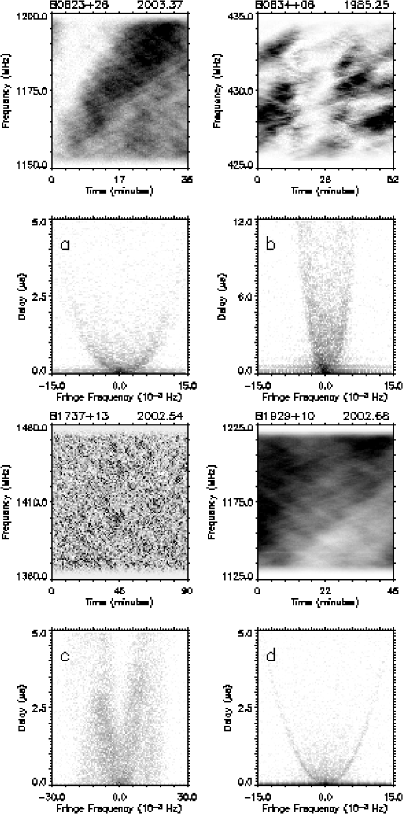
Figure 1: Primary and secondary spectrum pairs are shown for 4 pulsars that exhibit the scintillation arc phenomenon. The grayscale for the primary spectrum is linear in flux density. For the secondary spectrum, the logarithm of the power is plotted, and the grayscale extends from 3 dB above the noise floor to 5 dB below the maximum power level. The dispersion measures of these pulsars range from 3.2 to 48.4 pc cm^-3 and the scattering measures range from $10^{-4.5}$ to $10^{-3.6}$ kpc m^-20/3, with PSR B1929+10 and PSR B0823+26 representing the extremes in scattering measure. The data shown here and in Figures 2-3 were obtained from the Arecibo Observatory.

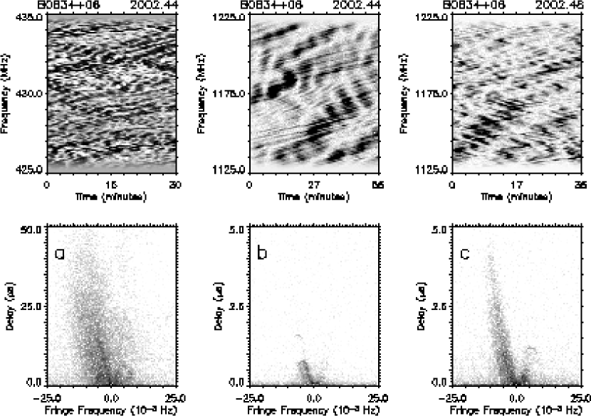
Figure 2: Three observations of PSR B0834+06 taken within two weeks of each other. The asymmetry with respect to the conjugate time axis is present, in the same sense, in all three observations. The broad power distribution at 430 MHz in (a) is much sharper one day later at 1175 MHz ($b$); however a more diffuse component has returned 14 days later ($c$). Note that the scales for the delay axis in ($b$) and ($c$) differ from that in ($a$). The inverted parabolic arclets noticeable in panels $b$ and $c$ are a common form of substructure for this and several other pulsars.

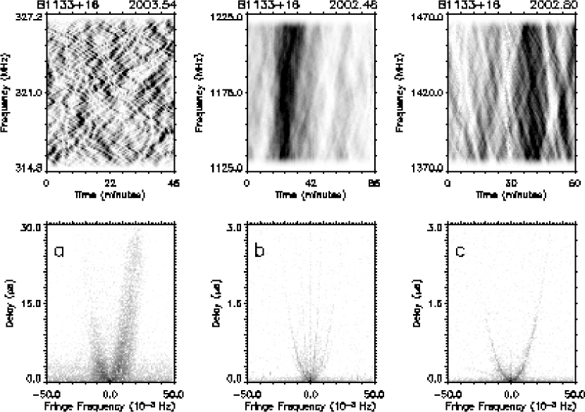
Figure 3: One of the pulsars in our sample, PSR B1133+16, shows multiple scintillation arcs on occasion. The broad, asymmetric power distribution in ($a$) has numerous arclets at 321 MHz. Panels ($b$) and ($c$) are at frequencies above 1 GHz. Panel ($b$) shows two clear arcs (along with a vertical line at $f_{\rm t}$ due to narrowband RFI and the sidelobe response of power near the origin). Four months later($c$), only the outer of these two arcs – widened by the $a\propto\nu^{-2}$ scaling – is visible.

3 Theory of Secondary Spectra and Scintillation Arcs

3.1 A Simple Theory

Though the parabolic arc phenomenon is striking and unexpected, it can be understood in terms of a simple model based on a “thin screen” of ionized gas containing fluctuations in electron density on a wide range of scales. Incident radiation is scattered by the screen and then travels through free space to the observer, at whose location radiation has a distribution in angle of arrival. The intensity fluctuations are caused by interference between different components of the angular spectrum whose relative phases increase with distance from the screen. Remarkably, we find that the arcs can be explained solely in terms of phase differences from geometrical path lengths. The phenomenon can equally well be described, using the Fresnel-Kirchoff diffraction integral, by spherical waves originating at a pair of points in the screen interfering at the observer having traveled along different geometric paths. Thus, though the screen is dispersive, the arcs arise simply from diffraction and interference. Dispersion and refraction in the screen will likely alter the shapes of the arcs, though we do not analyze these effects in this paper.

To get interference, the screen must be illuminated by a radiation field of high spatial coherence, i.e. radiation from a point-like source. The source can be temporally incoherent because the different components of the temporal Fourier transform each contribute nearly identical interference patterns, as in interferometry. Two components of the angular spectrum arriving from directions ${\mbox{\boldmath$\theta$}}_{1}$ and ${\mbox{\boldmath$\theta$}}_{2}$ interfere to produce a two-dimensional fringe pattern whose phase varies slowly with observing frequency. The pattern is sampled in time and frequency as the observer moves through it, creating a sinusoidal fringe pattern in the dynamic spectrum. The fringe appears as a single Fourier component in the secondary spectrum. Under the small-angle scattering of the ISM its $f_{\nu}$ coordinate is the differential geometric delay $\propto\theta_{2}^{2}-\theta_{1}^{2}$ and its $f_{\rm t}$ coordinate is the fringe rate $\propto{\bf V_{\perp}}\cdot({\mbox{\boldmath$\theta$}}_{2}-{\mbox{\boldmath$\theta$}}_{1})$, where ${\bf V_{\perp}}$ is an appropriate transverse velocity (see below). A quadratic relationship $f_{\nu}$ to $f_{\rm t}$ results naturally from their quadratic and linear dependences on the angles. When one of the interfering waves is undeviated (e.g. ${\mbox{\boldmath$\theta$}}_{1}=0$) we immediately get the simple parabola $f_{\nu}\propto f_{\rm t}^{2}$. When the scattering is weak there will be a significant undeviated contribution resulting in a simple parabolic arc. However, we also find that an arc appears in strong scattering due to the interference of waves contained within the normal scattering disc with a faint halo of waves scattered at much larger angles. The faint halo exists only for scattering media having wavenumber spectra less steep than (wavenumber)^-4, including the Kolmogorov spectrum.

While the relation of $f_{\nu}$ to time delay is well known through the Fourier relationship of the pulse broadening to the radio spectrum intensity scintillation, the physical interpretation of $f_{\rm t}$ can be viewed in several ways besides the fringe rate. Scintillation versus time is often Fourier analyzed into a spectrum versus frequency ($f_{\rm t}$) in Hz; in turn this is simply related to spatial wavenumber $f_{\rm t}={\mbox{\boldmath$\kappa$}}\cdot{\bf V_{\perp}}/(2\pi)$ and hence to angle of arrival (${\mbox{\boldmath$\kappa$}}=k{\mbox{\boldmath$\theta$}}$). It can also be thought of as the beat frequency due to the different Doppler shifts of the two scattered waves. Thus the secondary spectrum can be considered as a differential delay-Doppler spectrum , similar to that measured in radar applications.

3.2 Screen Geometry

In this section we discuss the relationship between the scattered image and the secondary spectrum $S_{2}$. Later, in §5, we obtain the relation more rigorously by deriving $S_{2}$ as a fourth moment of the electric field. Explicit results can be obtained in the limits of strong and weak scintillation, as shown in Appendices C and D. We find that the weak scintillation result is simpler, being a second moment of the electric field since it only involves the interference of scattered waves with the unscattered field. However, pulsars are typically observed in strong scintillation, and the strong scintillation limit gives exactly the same result as in the approximate theory (Eq. 8) used below. So we now apply the approximate theory to spherical waves from a pulsar scattered by a thin screen.

Consider the following geometry: a point source at $z=0$, a thin screen at $z={D_{\rm s}}$ and an observer at $z=D$. For convenience, we define $s={D_{\rm s}}/D$. The screen changes only the phase of incident waves, but it can both diffract and refract radiation from the source. For a single frequency emitted from the source two components of the angular spectrum at angles ${\mbox{\boldmath$\theta$}}_{1}$, ${\mbox{\boldmath$\theta$}}_{2}$ (measured relative to the direct path) sum and interfere at the observer’s location with a phase difference ${\Phi}$. The resulting intensity is $I=I_{1}+I_{2}+2\sqrt{I_{1}I_{2}}\cos{\Phi}$ where $I_{1}$ and $I_{2}$ are the intensities from each component (e.g. Cordes & Wolszczan 1986). The total phase difference ${\Phi}=\Phi_{\rm g}+\phi$, includes a contribution from geometrical path-length differences $\Phi_{\rm g}$ and from the screen phase, $\phi$, which can include both small and large-scale structures that refract and diffract radiation. Expanding ${\Phi}$ to first order in time and frequency increments, $\delta t$ and $\delta\nu$, the phase difference is

$${\Phi}=\Phi_{0}+2\pi(f_{t}\delta t+f_{\nu}\delta\nu),$$ (1)

where $\delta\nu=\nu-\nu_{0}$, $\delta t=t-t_{0}$ and $t_{0},\nu_{0}$ define the center of the observing window; $f_{t}=(1/2\pi)\partial_{t}{\Phi}$ is the fringe rate or differential Doppler shift, and $f_{\nu}=(1/2\pi)\partial_{\nu}{\Phi}$ is the differential group delay. In general $\Phi$ includes both a geometrical path-length difference and a dispersive term. At the end of §5.2 we consider the effects of dispersion, but in many cases of pulsar scintillation it can be shown that the dispersive term can be ignored. We proceed to retain only the geometric delays and obtain results (Appendix A) that were reported in Paper 1:

$$f_{\nu} = \left[\frac{D(1-s)}{2\,c\,s}\right]\left({\mbox{\boldmath$\theta$}}_{2}^{2}-{\mbox{\boldmath$\theta$}}_{1}^{2}\right)$$ (2)

$$f_{t} = \left(\frac{1}{\lambda\,s}\right)({\mbox{\boldmath$\theta$}}_{2}-{\mbox{\boldmath$\theta$}}_{1})\cdot{\bf V_{\perp}}.$$ (3)

Here $\lambda$ is the wavelength at the center of the band, $s={D_{\rm s}}/D$, and ${\bf V_{\perp}}$ is the velocity of the point in the screen intersected by a straight line from the pulsar to the observer, given by a weighted sum of the velocities of the source, screen and observer (e.g. Cordes & Rickett 1998):

$${\bf V_{\perp}}=(1-s){\bf{V_{\rm p}}_{\perp}}+s{\bf{V_{\rm obs}}_{\perp}}-{\bf{V_{\rm screen}}_{\perp}}.$$ (4)

It is also convenient to define an effective distance ${D_{\rm e}}$,

$${D_{\rm e}}=Ds(1-s)\;.$$ (5)

The two-dimensional Fourier transform of the interference term $\cos{\Phi}(\delta\nu,\delta t)$ is a pair of delta functions placed symmetrically about the origin of the delay fringe-rate plane. The secondary spectrum at ($f_{\nu},f_{\rm t}$) is thus the summation of the delta functions from all pairs of angles subject to Eq. 2 & 3, as we describe in the next section.

3.3 Secondary Spectrum in Terms of the Scattered Brightness

In this section we examine how the form of the secondary spectrum varies with the form assumed for the scattered image, without considering the associated physical conditions in the medium. We postpone to §5 a discussion of the scattering physics and the influence of the integration time. The integration time is important in determining whether the scattered brightness is a smooth function or is broken into speckles as discussed by Narayan & Goodman (1989). This in turn influences whether the secondary spectrum takes a simple parabolic form or becomes fragmented.

We analyze an arbitrary scattered image by treating its scattered brightness distribution, $B({\mbox{\boldmath$\theta$}})$, as a probability density function (PDF) for the angles of scattering. In the continuous limit the secondary spectrum is the joint PDF of $f_{\nu},f_{\rm t}$ subject to the constraints of Eq. (2 & 3). It is convenient to use dimensionless variables for the delay and fringe rate:

$$p = {\mbox{\boldmath$\theta$}}_{2}^{2}-{\mbox{\boldmath$\theta$}}_{1}^{2}=\left[\frac{2cs}{D(1-s)}\right]f_{\nu},$$ (6)

$$q = ({\mbox{\boldmath$\theta$}}_{2}-{\mbox{\boldmath$\theta$}}_{1})\cdot{\mbox{\boldmath$\hat{V}_{\perp}$}}=\left(\frac{\lambda s}{{V_{\perp}}}\right)f_{\rm t},$$ (7)

where $\hat{V}_{\perp}$ is a two-dimensional unit vector for the transverse effective velocity. It is also useful to normalize angles by the characteristic diffraction angle, ${\theta_{\rm d}}$, so in some contexts discussed below $\theta\to\theta/{\theta_{\rm d}}$, in which case $p\to f_{\nu}/\tau_{\rm d}$ and $q\to 2\pi\Delta t_{\rm d}f_{\rm t}$, where $\tau_{\rm d}$ is the pulse broadening time and $\Delta t_{\rm d}$ is the diffractive scintillation time. The secondary spectrum is then given by an integral of the conditional probability $\delta(p-{\overline{p}})\delta(q-{\overline{q}})$ for a given pair of angles multiplied by the PDFs of those angles,

$${S_{2}}(p,q)=\int\int d{\mbox{\boldmath$\theta$}}_{1}\,d{\mbox{\boldmath$\theta$}}_{2}\,{\mbox{$B$}}({\mbox{\boldmath$\theta$}}_{1}){\mbox{$B$}}({\mbox{\boldmath$\theta$}}_{2})\delta(p-{\overline{p}})\delta(q-{\overline{q}}),$$ (8)

where ${\overline{p}},{\overline{q}}$ are the values of $p,q$ for particular values of ${\mbox{\boldmath$\theta$}}_{1,2}$ as given in Eq. 6 and 7. In Appendix C, Eq. 8 is derived formally from the ensemble average in the limit of strong diffractive scattering.

The secondary spectrum is symmetric through the origin ($p\to-p$ and $q\to-q$). Eq. (8) shows that it is essentially a distorted autocorrelation of the scattered image. With no loss of generality we simplify the analysis by taking the direction of the velocity to be the $x$ direction. The four-fold integration in Eq. 8 may be reduced to a double integral by integrating the delta functions over, say, ${\mbox{\boldmath$\theta$}}_{2}$ to obtain

$${S_{2}}(p,q)=\frac{1}{2}\int\int d{\theta_{1}}_{x}\,d{\theta_{1}}_{y}\,H(U)U^{-1/2}{\mbox{$B$}}({\theta_{1}}_{x},{\theta_{1}}_{y})\left[{\mbox{$B$}}(q+{\theta_{1}}_{x},\sqrt{U})+{\mbox{$B$}}(q+{\theta_{1}}_{x},-\sqrt{U})\right],$$ (9)

where

$$U\equiv p-q^{2}-2q{\theta_{1}}_{x}+{\theta_{1}}_{y}^{2}$$ (10)

and $H(U)$ is the unit step function. With this form, the integrand is seen to maximize at the singularity $U=0$, which yields a quadratic relationship between $p$ and $q$. For an image offset from the origin by angle ${\mbox{\boldmath$\theta$}}_{0}$, e.g. ${\mbox{$B$}}({\mbox{\boldmath$\theta$}})\to{\mbox{$B$}}({\mbox{\boldmath$\theta$}}-{\mbox{\boldmath$\theta$}}_{0})$, the form for ${S_{2}}$ is similar except that $U=p-q^{2}-2q(\theta_{1x}+{\theta}_{0x})+({\theta_{1}}_{y}+{\theta}_{0y})^{2}$ and the ${\theta}_{y}$ arguments of $B$ in square brackets in Eq. 9 become $\pm\sqrt{U}-{\theta}_{0y}$. The integrable singularity at $U=0$ makes the form of Eq. 9 inconvenient for numerical evaluation. In Appendix B we use a change of variables to avoid the singularity, giving form (Eq. B4) that can be used in numerical integration. However, this does not remove the divergence of ${S_{2}}$ at the origin $p=q=0$. In Appendix B we show that inclusion of finite resolutions in $p$ or $q$, which follow from the finite extent of the orignal dynamic spectrum in time and frequency, avoids the divergence at the origin, emphasizing that the dynamic range in the secondary spectrum is strongly influenced by resolution effects.

The relation $p=q^{2}$ follows from the singularity $U=0$ after integration over angles in Eq. 9 and is confirmed in a number of specific geometries discussed below. This relation becomes $f_{\nu}=af_{\rm t}^{2}$ in dimensional units, with

$$a=\frac{Ds(1-s)}{2c}\left(\frac{\lambda}{{V_{\perp}}}\right)^{2}=0.116\left[\frac{s(1-s)}{1/4}\right]D_{\rm kpc}\nu^{-2}V_{100}^{2}\,{\rm sec^{-3}},\,$$ (11)

where ${V_{\perp}}=100\,{\rm km\,s^{-1}}\,V_{100}$ and $\nu$ is in GHz. For screens halfway between source and observer ($s=1/2)$, this relation yields values for $a$ that are consistent with the arcs evident in Figures 1-3 and also shown in Papers 1-3. As noted in Paper 1, $a$ does not depend on any aspect of the scattering screen save for its fractional distance from the source, $s$, and it maximizes at $s=1/2$ for fixed ${V_{\perp}}$. When a single arc occurs and other parameters in Eq. 11 are known, $s$ can be determined to within a pair of solutions that is symmetric about $s=1/2$. However, when ${V_{\perp}}$ is dominated by the pulsar speed, $s$ can be determined uniquely (c.f. Paper 1).

3.4 Properties of the Secondary Spectrum

To determine salient properties of the secondary spectrum that can account for many of the observed phenomena, we consider special cases of images for which Eq. 8 can be evaluated. As noted above the effects of finite resolution are important both observationally and computationally and are discussed in Appendix B.

3.4.1 Point Images

A point image produces no interference effects, so the secondary spectrum consists of a delta function at the origin, $(p,q)=(0,0)$. Two point images with amplitudes $a_{1}$ and $a_{2}$ produce fringes in the dynamic spectrum, which give delta functions of amplitude $a_{1}a_{2}$ at position given by Eq. 6 and 7 and its counterpart reflected through the origin and also a delta function at the origin with amplitude $1-2a_{1}a_{2}$. Evidently, an assembly of point images gives a symmetrical pair of delta functions in $p,q$ for each pair of images.

3.4.2 One-dimensional Images

Arc features can be prominent for images elongated in the direction of the effective velocity. Consider an extreme but simple case of a one dimensional image extended along the $x$ axis only

$${\mbox{$B$}}({\mbox{\boldmath$\theta$}})=g(\theta_{x})\delta(\theta_{y}),$$ (12)

and where $g$ is an arbitrary function. The secondary spectrum is

$${S_{2}}(p,q)=\left(2|q|\right)^{-1}g\left(\frac{p-q^{2}}{2q}\right)g\left(\frac{p+q^{2}}{2q}\right).$$ (13)

By inspection, parabolic arcs extend along $p=\pm q^{2}$ with amplitude ${S_{2}}\propto g(q)/|q|$ along the arc, becoming wider in $p$ at large $|q|$. However, for the particular case where $g$ is a Gaussian function, the product of the $g$ functions in Eq.  (13) $\propto\exp[-(p^{2}+q^{4})/2q^{2}]$, which cuts off the arcs very steeply (see §4.1). For images with slower fall offs at large angles, the arc features can extend far from the origin. For the same image shape elongated transverse rather than parallel to $x$, inspection of Eq. 7 - 8 indicates that ${S_{2}}(p,q)\propto\delta(q)$, so there is only a ridge along the $q$-axis. These examples suggest that prominent arcs are expected when images are aligned with the direction of the effective velocity, as we confirm below for more general image shapes.

3.4.3 Images with a Point and an Extended Component

Consider a scattered image consisting of a point source at ${\mbox{\boldmath$\theta$}}_{p}$ and an arbitrary, two-dimensional image component, $g({\mbox{\boldmath$\theta$}})$,

$${\mbox{$B$}}({\mbox{\boldmath$\theta$}})=a_{1}\delta({\mbox{\boldmath$\theta$}}-{\mbox{\boldmath$\theta$}}_{p})+a_{2}g({\mbox{\boldmath$\theta$}}).$$ (14)

The secondary spectrum consists of the two self-interference terms from each image component and cross-component terms of the form

$$\Delta{S_{2}}(p,q)=\frac{1}{2}a_{1}a_{2}U^{-1/2}H(U)\sum_{\pm}g(q+{\theta_{p}}_{x},\pm\sqrt{U})+S.O.,$$ (15)

where $U=p-q^{2}-2q{\theta_{p}}_{x}+{\theta_{p}}_{y}^{2}$, $H(U)$ is the unit step function and “S.O.” implies an additional term that is symmetric through the origin, corresponding to letting $p\to-p$ and $q\to-q$ in the first component. A parabolic arc is defined by the $H(U)U^{-1/2}$ factor. As $U\to 0$ the arc amplitude is $a_{1}a_{2}U^{-1/2}g(q+{\theta}_{p_{x}},0)$. Considering $g$ to be centered on the origin with width ${W_{\rm g}}_{x}$ in the $x$ direction, the arc extends to $|q+{\theta_{p}}_{x}|\lesssim{W_{\rm g}}_{x}/2$. Of course if the point component has a small but non-zero diameter, the amplitude of the arc would be large but finite. If the point is at the origin, the arc is simply $p=q^{2}$ as already discussed. In such cases Eq. 15 can be inverted to estimate $g({\mbox{\boldmath$\theta$}})$ from measurements of $\Delta{S_{2}}$. The possibility of estimating the two-dimensional scattered brightness from observations with a single dish is one of the intriguing aspects of the arc phenomenon.

With the point component displaced from the origin, the apex of the parabola is shifted from the origin to

$$(p,q)_{\rm apex}=(-\theta_{p}^{2},-{\theta_{p}}_{x}).$$ (16)

By inspection of Eq. 15, the condition $U=0$ implies that the arc is dominated by contributions from image components scattered parallel to the velocity vector at angles ${\mbox{\boldmath$\theta$}}=(q+{\theta}_{p_{x}},0)$. Thus images elongated along the velocity vector produce arcs enhanced over those produced by symmetric images. This conclusion is general and is independent of the location, ${\mbox{\boldmath$\theta$}}_{p}$, of the point component.

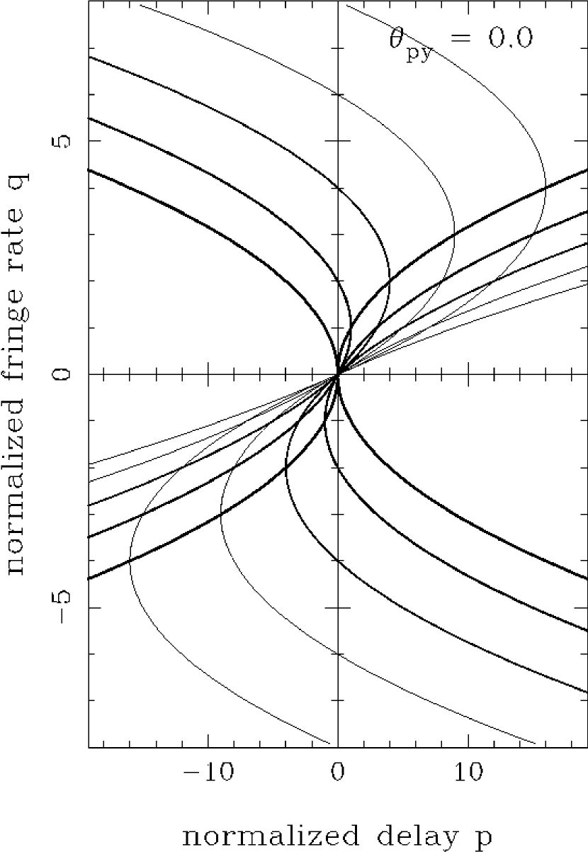
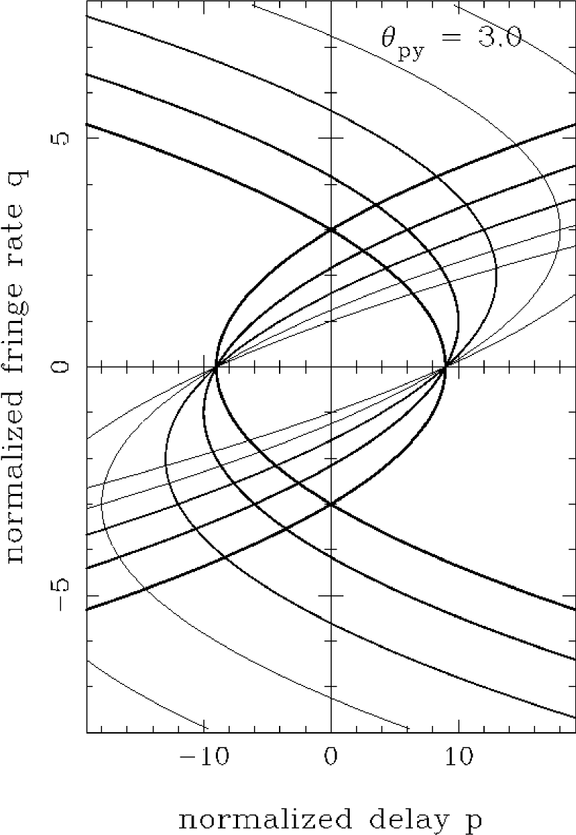
Figure 4: Trajectories for parabolic arcs due to interference between a point component at $(\theta_{px},\theta_{py})$ with an extended distribution. The curves are for five values of normalized $\theta_{px}$ (0 for thickest line to 4 for thinnest line). Left panel: for $\theta_{py}=0$ the parabolas have apexes of the reverse arcs lying along $p=q^{2}$. Right panel: for $\theta_{py}=3$, the apexes are inside $p=q^{2}$.

Figure 4 shows parabolic arc lines ($U=0$) for various assumed positions for the point component. Eq.16 gives a negative delay at the apex, but since ${S_{2}}$ is symmetric about the origin, there is also a parabola with a positive apex, but with reversed curvature. When ${\theta}_{p_{y}}=0$ the apex must lie on the basic arc $p=q^{2}$ (left panel), and otherwise the apex must lie inside it (right panel). Such features suggest an explanation for the reversed arclets that are occasionally observed, as in Figure 2. We emphasize that the discussion here has been restricted to the interference between a point and an extended component, and one must add their self-interference terms for a full description.

The foregoing analysis can, evidently, be applied to a point image and an ensemble of subimages. The general nature of ${S_{2}}$ is similar in that it is enhanced along the curve where $U=0$ which enhances subimages lying along the velocity vector.

4 Secondary Spectra for Cases Relevant to the Interstellar Medium

We now compute the theoretical secondary spectrum for various simple scattered brightness functions commonly invoked for interstellar scattering. The computations include self-interference and also the finite resolution effects, discussed in Appendix B.

4.1 Elliptical Gaussian Images

Measurements of angular broadening of highly scattered OH masers (Frail et al. 1994), Cyg X-3 (Wilkinson et al. 1994), pulsars (Gwinn et al. 1993), and AGNs (e.g. Spangler & Cordes 1988; Desai & Fey 2001) indicate that the scattering is anisotropic and, in the case of Cyg X-3, consistent with a Gaussian scattering image, which probably indicates diffractive scales smaller than the “inner scale” of the medium. Dynamic spectra cannot be measured for such sources because the time and frequency scales of the diffractive scintillations are too small and are quenched by the finite source size. However, some less scattered pulsars may have measurable scintillations that are related to an underlying Gaussian image.

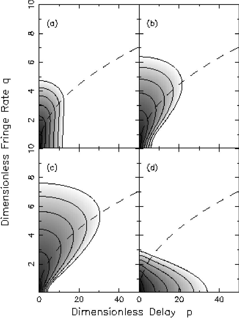
Figure 5: Secondary spectra corresponding to Gaussian scattered images with different ellipticities and orientations: (a) a circular Gaussian image; (b) an elliptical Gaussian with axial ratio of 2 elongated along the $x$ axis; (c) an axial ratio of 3 elongated along the $x$ axis; and (d) an axial ratio of 3 elongated along the $y$ axis. The contour separation is one decade and the outermost contour is 6 decades from the peak of the secondary spectrum. The dashed line shows the parabola, $p=q^{2}$.

The secondary spectrum for an elliptical Gaussian image cannot be solved analytically, although Eq. B4 can be reduced to a one dimensional integral which simplifies the numerical evaluation. Figure 5 shows some examples. The upper left hand panel is for a single circular Gaussian image. It does not exhibit arc-like features, although it “bulges” out along the dashed arc-line ($p=q^{2}$). Upper right is for an elliptical Gaussian image with a 2:1 axial ratio parallel to the velocity vector. The 3:1 case (lower left) shows the deep “valley” along the delay ($p$) axis, which is characteristic of images elongated parallel to the velocity. Such deep valleys are frequently seen in the observations and provide evidence for anisotropic scattering. Notice, however, that the secondary spectrum can be strong outside of the arc line, where the contours become parallel to the $p$-axis. Inside the arc-line the contours follow curves like the arc-line. The 3:1 case with the major axis transverse to the velocity (lower right) shows enhancement along the delay axis with no bulging along the arc-line.

4.2 Media with Power-Law Structure Functions

Here we consider brightness distributions associated with wavenumber spectra having a power-law form. For circularly symmetric scattering, the phase structure function depends only on the magnitude of the baseline so the visibility function is $\Gamma(b)=\exp[-\frac{1}{2}D_{\phi}(b/s_{0})]$. A suitable power-law form for the structure function is $D_{\phi}(b)=(b/s_{0})^{\alpha}$, where $s_{0}$ is the spatial scale of the intensity diffraction pattern, defined such that $|\Gamma(s_{0})|^{2}=e^{-1}$ (e.g. Cordes & Rickett 1998). The corresponding image is

$$B(\theta)=2\pi\int_{0}^{\infty}b\,db\,\Gamma(b)J_{0}(2\pi b\theta/\lambda),$$ (17)

where $J_{0}$ is the Bessel function. Computations are done in terms of an image normalized so that $B(0)=1$, a scaled baseline $\eta=b/s_{0}$, and a scaled angular coordinate $\psi=\theta/{\theta_{\rm d}}$, where ${\theta_{\rm d}}=(ks_{0})^{-1}$ is the scattered angular width.

4.2.1 Single-slope Power Laws

First we consider phase structure functions of the form $D_{\phi}(b)\propto b^{\alpha}$. The corresponding wavenumber spectra $\propto({\rm wavenumber})^{-\beta}$ with indices $\beta=\alpha+2$ for $\beta<4$ (e.g. Rickett 1990). Figure 6 (left-hand panel) shows one-dimensional slices through the images associated with four different values of $\alpha$, including $\alpha=2$, which yields a Gaussian-shaped image. The corresponding secondary spectra are shown in Figure 7. Arcs are most prevalent for the smallest value of $\alpha$, become less so for larger $\alpha$, and are nonexistent for $\alpha=2$. Thus the observation of arcs in pulsar secondary spectra rules out the underlying image having the form of a symmetric Gaussian function, and so puts an upper limit on an inner scale in the medium.

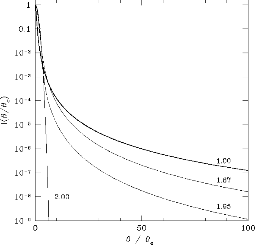
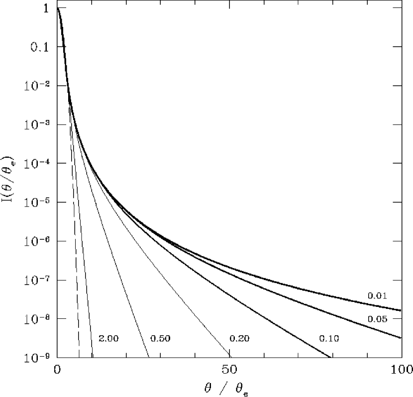
Figure 6: Left: Slices through circularly symmetric images associated with phase structure functions $D_{\phi}\propto b^{\alpha}$ for $\alpha=$ 1,1.67,1.95 and 2 (thickest to thinnest lines and as labelled). The $\alpha=2$ case corresponds to an image that is Gaussian in form. Right: Slices through circularly symmetric images for a Kolmogorov wavenumber spectrum with different fractional inner scales, $\zeta$, as defined in the text and as labelled for each curve. The dashed curve shows a Gaussian image with the same e-folding width as the Kolmogorov curves.

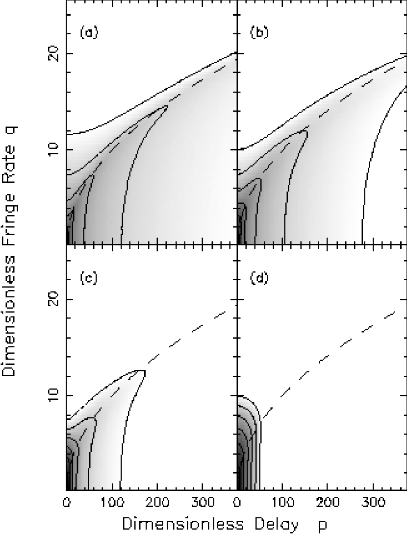
Figure 7: Secondary spectra corresponding to the image cases shown in the left panel of Figure 6. (a) $\alpha=1.0$; (b) $\alpha=1.67$; (c) $\alpha=1.95$; (d) $\alpha=2.0$. The contour separation is one decade and the outermost contour is 6 decades from the peak of the secondary spectrum. The dashed line shows the parabola, $p=q^{2}$.

Arcs for all of the more extended images, including the $\alpha=1.95$ case, appear to be due to the interference of the central “core” ($\psi<1$) with the weak “halo” ($\psi\gg 1$) evident in Figure 6 (both panels). This interpretation is confirmed by the work of Codona et al.   (1986). Their Eq. (43) gives the cross spectrum of scintillations between two frequencies in the limit of large wavenumbers in strong scintillation. When transformed, the resulting secondary spectrum is exactly the form of an unscattered core interfering with the scattered angular spectrum.

The halo brightness at asymptotically large angles scales as $\psi^{-(\alpha+2)}$. We can use this in Eq. 15 with the undeviated core as the point component (${\mbox{\boldmath$\theta$}}_{p}=0$) to find ${S_{2}}(p,q)$ far from the origin:

$${S_{2}}(p,q)\propto p^{-(\alpha+2)/2}|p-q^{2}|^{-1/2}\quad\quad p>q^{2}.$$ (18)

Along the $p$-axis, ${S_{2}}(p,0)\propto p^{-(\alpha+3)/2}$.

4.2.2 Kolmogorov Spectra with an Inner Scale

A realistic medium is expected to have a smallest (“inner”) scale in its density fluctuations. Depending on its size, the inner scale may be evident in the properties of pulsar scintillations and angular broadening. Angular broadening measurements, in particular, have been used to place constraints on the inner scale for heavily scattered lines of sight (Moran et al. 1990; Molnar et al. 1995; Wilkinson et al. 1994; Spangler & Gwinn 1990). For scintillations, the inner scale can alter the strength of parabolic arcs, thus providing an important method for constraining the inner scale for lines of sight with scattering measures much smaller than those on which angular broadening measurements have been made. We consider an inner scale, $\ell_{1}$, that cuts off a Kolmogorov spectrum and give computed results in terms of the normalized inner scale $\zeta=\ell_{1}/s_{0}$. The structure function scales asymptotically as $D_{\phi}\propto b^{2}$ below $\ell_{1}$ and $\propto b^{5/3}$ above.

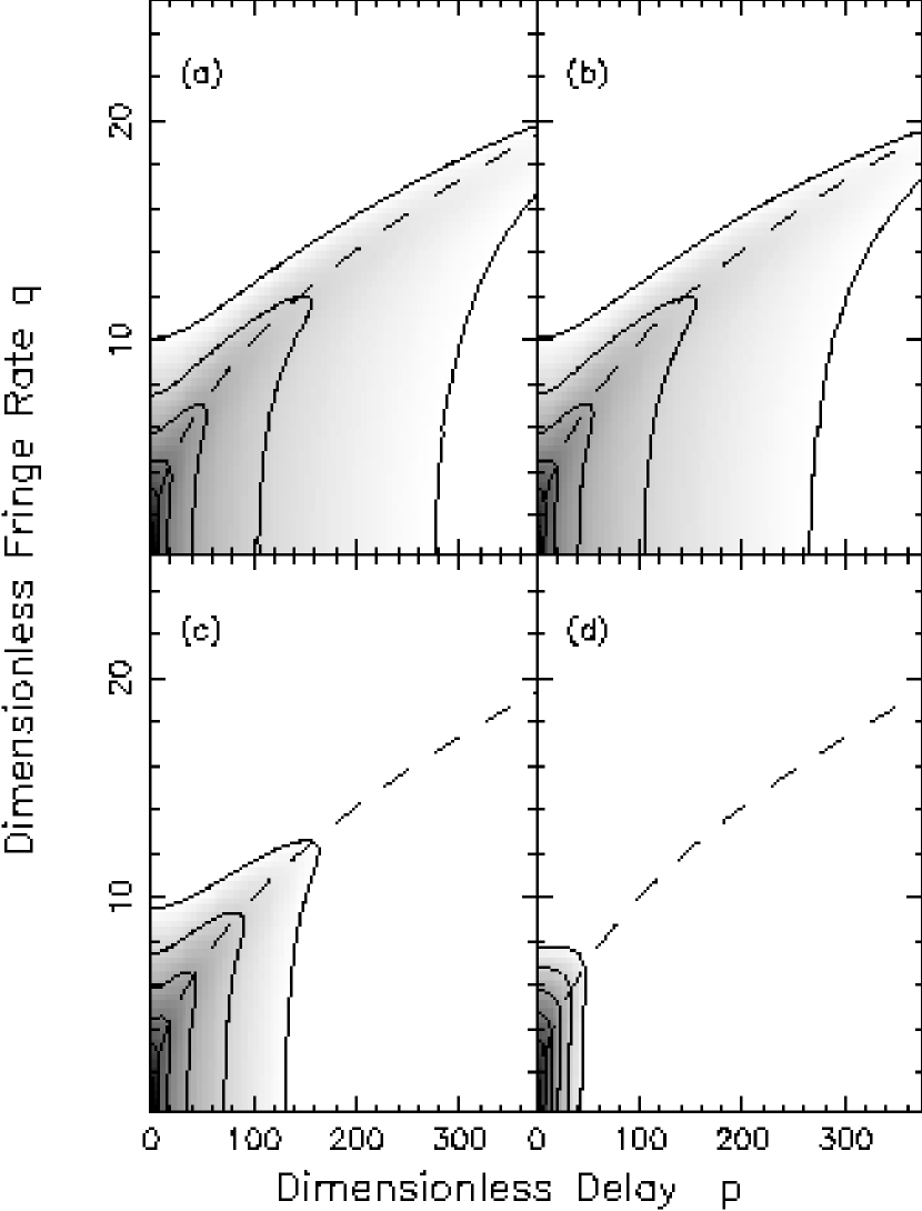
Figure 8: Secondary spectra corresponding to some of the image cases shown in the right panel of Figure 6. (a) $\zeta=0.01$; (b) $\zeta=0.1$; (c) $\zeta=0.5$; (d) $\zeta=2.0$. The contour separation is one decade and the outermost contour is 6 decades from the peak of the secondary spectrum. The dashed line shows the parabola, $p=q^{2}$.

In the right panel of Figure 6, we show one-dimensional images for six values of $\zeta$. For $\zeta\ll 1$, the inner scale is negligible and the image falls off relatively slowly at large $\psi$, showing the extended halo $\propto\psi^{-11/3}$, as for the Kolmogorov spectrum with no inner scale. For $\zeta=2$, the image falls off similarly to the shown Gaussian form and thus does not have an extended halo. Secondary spectra are shown in Figure 8 for four values of inner scale. As expected, the arcs are strongest for the case of negligible inner scale and become progressively dimmer and truncated as $\zeta$ increases and the image tends toward a Gaussian form. The appearance of strong arcs in measured data indicates that the the inner scale must be much less than the diffraction scale, or $\ell_{1}\ll 10^{4}$ km, for lines of sight to nearby pulsars, such as those illustrated in Figures 1-3.

4.2.3 Anisotropic Kolmogorov Spectrum

Figure 9 shows the results for an anisotropic Kolmogorov spectrum with a 3:1 axial ratio ($R=1/3$) for different orientation angles of the image with respect to the velocity. In the upper left panel the scattered image is elongated parallel to the velocity, and the arc is substantially enhanced with a deep valley along the $p$-axis. As the orientation tends toward normal with respect to the velocity in the other panels, the arc diminishes and essentially disappears. The deep valley in the parallel case occurs because $q={\theta_{x}}_{2}-{\theta_{x}}_{1}=0$ along the $p$-axis, so $p={\theta_{y}^{2}}_{2}-{\theta_{y}^{2}}_{1}$, in which case the secondary spectrum falls steeply like the brightness distribution along its narrow dimension. By comparison, along the arc itself, the secondary spectrum probes the wide dimension and thus receives greater weight. Taking the asymptotic brightness at large angles, $B\propto(R\psi_{x}^{2}+\psi_{y}^{2}/R)^{-11/6}$ for interference with the undeviated core in Eq. 15 we obtain:

$${S_{2}}(p,q)\propto[q^{2}(R-1/R)+p/R]^{-11/6}[p-q^{2}]^{-1/2}\quad\quad p>q^{2}.$$ (19)

Along the $p$-axis the amplitude of the secondary spectrum in Eq. 19 tends asymptotically to $\propto p^{-7/3}$.

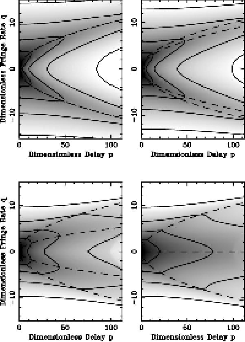
Figure 9: Secondary spectra computed from the brightness distribution in the diffractive limit due to an anisotropic Kolmogorov phase spectrum. The axial ratio is 3:1 with four angles of orientation. In the upper left panel, the brightness distribution is extended parallel to the velocity; upper right at 30 $\deg$; lower left at 60 $\deg$; and lower right at 90 $\deg$. Contours are at decade intervals. The solid curves are $p=q^{2}$ and $p=(q\sec\phi)^{2}$, corresponding to arcs for idealized circular and linear brightness functions.

5 Scattering Theory

5.1 Derivation of the Secondary Spectrum

In prior sections we related $f_{\nu}$ and $f_{\rm t}$ to the angles of scattering through Eq. 2 and 3. The intensity of the scattered waves at each angle was represented by a scattered brightness function $B({\mbox{\boldmath$\theta$}})$ with little discussion of the scattering physics that relates $B({\mbox{\boldmath$\theta$}})$ to the properties of the ISM.

In discussing the scattering physics, we must consider the relevant averaging interval. Ensemble average results can be found in the limits of strong and weak scintillation, as we describe in Appendices C and D. In both cases the analysis depends on the assumption of normal statistics for the scattered field and the use of the Fresnel-Kirchoff diffraction integral to obtain a relation with the appropriate ensemble average $B({\mbox{\boldmath$\theta$}})$. However, for strong scattering we adopt the common procedure of approximating the observed spectrum by the ensemble average in the diffractive limit (after removal of the slow changes in pulse arrival time due to changing dispersion measure). In both cases $B({\mbox{\boldmath$\theta$}})$ is a smooth function of angle (except for the unscattered component in weak scintillation).

An instantaneous angular spectrum is a single realization of a random process. Thus it will exhibit “speckle”, i.e. the components of the angular spectrum are statistically independent having an exponential distribution. Goodman and Narayan (1989) called this the snapshot image, which is obtained over times shorter than one diffractive scintillation time ($\sim$minutes). However, we average the secondary spectrum over $\sim 1$ hour, which includes many diffractive scintillation timescales but is short compared to the time scale of refractive interstellar scintillation (RISS). Thus we need an image obtained from averaging over many diffractive times, which Goodman and Narayan refer to as the short-term average image. The short-term average image has some residual speckle but is less deeply modulated than the snapshot image. An approximate understanding of the effect of speckle in the image on the secondary spectrum is obtained from §3.4.3, by considering a single speckle as a point component that interferes with an extended component that represents the rest of the image. Thus each speckle can give rise to part of an arclet and multiple speckles will make an assembly of intersecting forward and reverse arclets.

While analytical ensemble average results for the secondary spectrum can be written in the asymptotic limits of weak and strong scattering, one must resort to simulation for reliable results in the intermediate conditions that are typical of many observations and in cases where a short-term average image is appropriate. We use the method and code described by Coles et al. (1995) and analyze the resulting diffraction pattern in the same manner as for the observations. We first create a phase screen at a single frequency whose wavenumber spectrum follows a specified (e.g. the Kolmogorov) form. We then propagate a plane wave through the screen and compute the resulting complex field over a plane at a distance $z$ beyond the screen. The intensity is saved along a slice through the plane of observation, giving a simulated time series at one frequency. The frequency is stepped, scaling the screen phase as for a plasma by the reciprocal of frequency, and the process is repeated. The assembly of such slices models a dynamic spectrum, which is then subject to the same secondary spectral analysis as used in the observations.

The results, while calculated for a plane wave source, can be mapped to a point source using the well-known scaling transformations for the screen geometry (i.e. $z\to{D_{\rm e}}$, as defined in Eq. 5). While the screen geometry is idealized, the simulation uses an electromagnetic calculation and properly accounts for dispersive refraction, diffraction and interference. Furthermore the finite size of the region simulated can approximate the finite integration time in the observations. A scalar field is used since the angles of scattering are extremely small and magnetionic effects are negligible in this context (c.f. Simonetti et al. 1984).

5.2 Interstellar Conditions Responsible for Arcs

In §3 we found two conditions that emphasize the arcs. The first is the interference between an undeviated wave and scattered waves, and the second is the enhancement of arcs when the waves are scattered preferentially parallel to the scintillation velocity. We now discuss how these conditions might occur.

5.2.1 Core-Halo Conditions.

The basic arc, $p=q^{2}$, is formed by interference of a core of undeviated or weakly deviated waves with widely scattered waves. There are two circumstances where a significant fraction of the total flux density can come from near ${\mbox{\boldmath$\theta$}}=0$. One is in strong scintillation, when the “central core” of the scattered brightness interferes with a wider low level halo, as discussed in §4.2 for a Kolmogorov density spectrum and other power-law forms with $\beta<4$ and neglible inner scale. In this case the core of the scattered brightness is not a point source, merely much more compact than the far-out halo radiation. Thus the arc is a smeared version of the form in Eq. 9, which has no power outside the basic arcline. Examples were shown in figures 7 and 8.

The other case is when the scattering strength is low enough that a fraction of the flux density is not broadened significantly in angle. The requirements on such an “unscattered core” are simply that the differential delay over the core must not exceed, say, a quarter of the wave period. Then the core is simply that portion of the brightness distribution in the first Fresnel zone, ${r_{\rm F}}$, and the electric-field components in the core sum coherently. Thus the core component can be significant even if the overall scattered brightness function is much wider than the first Fresnel zone.

The relative strength of the core to the remainder of the brightness distribution can be defined in term of the “strength of scintillation”. We define this as $m_{\rm B}$, the normalized rms intensity (scintillation index) under the Born approximation. It can be written in terms of the wave structure function $D_{\phi}(r)$, as ${m_{\rm B}^{2}}=0.77D_{\phi}({r_{\rm F}})$ with a simple Kolmogorov spectrum, where $D_{\phi}(r)=(r/s_{0})^{5/3}$, $s_{0}$ is the field coherence scale and ${r_{\rm F}}=\sqrt{{D_{\rm e}}/k}$ and $k=2\pi/\lambda$. Here ${\theta_{\rm d}}=1/ks_{0}$ defines the scattering angle. This gives ${m_{\rm B}^{2}}=0.77({r_{\rm F}}/s_{0})^{5/3}$; thus it is also related to the fractional diffractive bandwidth $\sim(s_{0}/{r_{\rm F}})^{2}$. Note that a distinction should be made between strength of scattering and strength of scintillation. For radio frequencies in the ISM we always expect that the overall rms phase perturbations will be very large compared to one radian, albeit over relatively large scales, which corresponds to strong scattering. In contrast strong scintillation corresponds to a change in phase of more than one radian across a Fresnel scale.

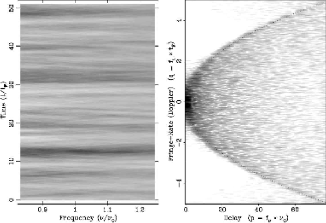
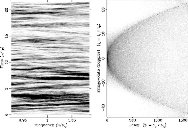
Figure 10: Primary and secondary spectra computed from simulations of plane wave incident on a phase screen with an isotropic Kolmogorov spectrum. Top: ${m_{\rm B}^{2}}=0.1$; Bottom: ${m_{\rm B}^{2}}=10$. On the left the primary dynamic spectrum has a grey scale proportional to the intensity from zero (white) to three times the mean (black). On the right the secondary spectrum has a grey scale proportional to the logarithm of the spectral density over a dynamic range of 5.5 decades (top) and 6.5 decades (bottom). Note the steep decrease outside the theoretical arcline ($p=q^{2}$, shown dotted).

In weak scintillation (but strong scattering) the fraction of the flux density in the core is $\sim(\theta_{\rm F}/{\theta_{\rm d}})^{2}=(s_{0}/{r_{\rm F}})^{2}\sim m_{\rm B}^{-2.4}$. Figure 10 (top panels) shows a simulation with ${m_{\rm B}^{2}}=0.1$, in which ${S_{2}}$ drops steeply outside the arc $p=q^{2}$. The analysis of Appendix D shows that in weak scintillation ${S_{2}}$ should be analyzed as a function of wavelength rather than frequency because the arcs are more clearly delineated when the simulations are Fourier analyzed versus wavelength. We have also simulated weak scintillation in a nondispersive phase screen and find similar arcs. In strong scintillation there is a small fractional range of frequencies and the distinction between wavelength and frequency becomes unimportant.

Figure 10 shows that the secondary spectrum in weak scintillation has a particularly well defined arc defined by a sharp outer edge. This is because it is dominated by the interference between scattered waves and the unscattered core, as described by Eq. (15) with a point component at the origin. We can ignore the mutual interference between scattered waves since they are much weaker than the core. The result is that the secondary spectrum is analogous to a hologram in which the unscattered core serves as the reference beam. The secondary spectrum can be inverted to recover the scattered brightness function using Eq. (15), which is the analog of viewing a holographic image. The inversion, however, is not complete in that there is an ambiguity in the equation between positive and negative values of $\theta_{y}$. Nevertheless, the technique opens the prospect of mapping a two-dimensional scattered image from observations with a single dish at a resolution of milliarcseconds.

As the scintillation strength increases the core becomes less prominent, and the parabolic arc loses contrast. However, we can detect arcs at very low levels and they are readily seen at large values of ${m_{\rm B}^{2}}$. Medium strong scintillation is shown in Figure 10 (bottom panels), which is a simulation of a screen with an isotropic Kolmogorov spectrum with ${m_{\rm B}^{2}}=10$ for which $s_{0}=0.22{r_{\rm F}}$. The results compare well with both the ensemble average, strong scintillation computations for a Kolmogorov screen in §4 and with several of the observations shown in Figure 1. We note that several of the observations in §2 show sharp-edged and symmetric parabolic arcs, which appear to be more common for low or intermediate strength of scintillation (as characterized by the apparent fractional diffractive bandwidth). This fits with our postulate that the arcs become sharper as the strength of scintillation decreases. In weak scintillation the Born approximation applies, in which case two or more arcs can be caused by two or more screens separated along the line of sight. We have confirmed this by simulating waves passing through several screens, each of which yields a separate arc with curvature as expected for an unscattered wave incident on each screen. This is presumably the explanation for the multiple arcs seen in Figure 3 for pulsar B1133+16.

In terms of normalized variables $p,q$ the half-power widths of ${S_{2}}$ are approximately unity in strong scattering and yet we can see the arcs out to $q\gg 1$. As we noted earlier this corresponds to scattering angles well above the diffractive angle ${\theta_{\rm d}}$, and so probes scales much smaller than those probed by normal analysis of diffractive ISS. Our simulations confirm that with an inner scale in the density spectrum having a wavenumber cutoff $\kappa_{\rm inner}$, the arc will be reduced beyond where $q\sim\kappa_{\rm inner}s_{0}$. However, to detect such a cut-off observationally requires very high sensitivity and a large dynamic range in the secondary spectrum.

5.2.2 Anisotropy, Arclets and Image Substructure

The enhancement in arc contrast when the scattering is extended along the direction of the effective velocity was discussed in §3. The enhancement is confirmed by comparing the ${m_{\rm B}^{2}}=10$ simulations in Figures 10 and 11.

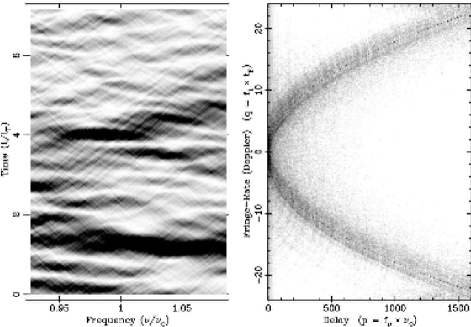
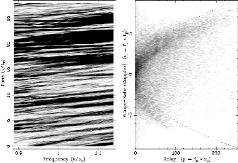
Figure 11: Simulations of a phase screen as in the bottom panel of Figure 10 with ${m_{\rm B}^{2}}=10$. Top: Anisotropic scattering (axial ratio 4:1 spectrum elongated along the velocity direction). The result is higher contrast in the arc, which is seen to consist of nearly parallel arclets and is crossed by equally fine scale reverse arcs. Bottom: Isotropic scattering with a linear refractive phase gradient of 2 radians per diffractive scale. The result is a shift in the parabola and an asymmetry in its strength.

In the anisotropic case the arc consists of finely-spaced parallel arcs which are in turn crossed by reverse arclets, somewhat reminiscent of the observations. The discussion of §3.4.3 suggests that these are caused by the mutual interference of substructure in the angular spectrum $B({\mbox{\boldmath$\theta$}})$. The question is, what causes the substructure? One possibility is that it is stochastic speckle-like substructure in the image of a scatter-broadened source. Alternatively, there could be discrete features in $B({\mbox{\boldmath$\theta$}})$, (“multiple images”) caused by particular structures in the ISM phase.

In our simulations, the screen is stochastic with a Kolmogorov spectrum and so it should have speckle but no deterministic multiple images. The diffractive scale, $s_{0}$, is approximately the size of a stationary phase point on the screen and, also, approximately the size of a constructive maximum at the observer plane. There are, thus, $\sim({r_{\rm F}}/s_{0})^{4}$ across the 2d scattering disk that contribute to an individual point at the observer plane. This large number of speckles ($\sim 400$ in these simulations) has the effect of averaging out details in the secondary spectrum, particularly in the isotropic scattering case.

The effect of anisotropy in the coherence scale is to broaden the image along one axis with respect to the other. An image elongated by a ratio of $R=\theta_{x}/\theta_{y}\approx s_{0,y}/s_{0,x}>1$ would have $N_{x}\approx({r_{\rm F}}/s_{0,x})^{2}$ speckes in the $x$-direction but only $N_{y}\approx({r_{\rm F}}/Rs_{0,x})^{2}$ in the $y$-direction. In short, the image would break into a line of many elliptical speckles (elongated in $y$) distributed predominantly along $x$. In comparing the anisotropic and isotropic simulations (upper Figure 11 and lower Figure 10), it appears that the arclets are more visible under anisotropy. We suggest that the changed substructure in the image is responsible. Substructure may consist of short-lived speckles or longer-lived multiple subimages whose relative contributions depend on the properties of the scattering medium. In the simulations the arclets appear to be independent from one realization to the next, as expected for a speckle phenomenon. However, in some of the observations arclets persist for as long as a month (see §2) and exhibit a higher contrast than in the simulation. These require long-lived multiple images in the angular spectrum and so imply quasi-deterministic structures in the ISM plasma.

In summary we conclude that the occasional isolated arclets (as in Figure 2) must be caused by fine substructure in $B({\mbox{\boldmath$\theta$}})$. Whereas some of these may be stochastic as in the speckles of a scattered image, the long lived arclets require the existence of discrete features in the angular spectrum, which cannot be part of a Kolmogorov spectrum. These might be more evidence for discrete structures in the medium at scales $\gtrsim 1$ AU, that have been invoked to explain fringing episodes (e.g. Hewish, Wolszczan & Graham 1985; Cordes & Wolszczan 1986; Wolszczan & Cordes 1987; Rickett, Lyne & Gupta 1997) and, possibly, extreme scattering events (ESEs) (Fiedler et al.  1987; Romani, Blandford & Cordes 1987) in quasar light curves.

5.2.3 Asymmetry in the Secondary Spectrum

As summarized in §2 the observed arcs are sometimes asymmetric as well as exhibiting reverse arclets (e.g. Figure 2). A scattered brightness that is asymmetric in $\theta_{x}$ can cause ${S_{2}}$ to become asymmetric in $q$. We do not expect a true ensemble average brightness to be asymmetric, but the existence of large scale gradients in phase will refractively shift the seeing image, with the frequency dependence of a plasma.

Simulations can be used to study refractive effects, as in Figure 11 (bottom panels), which shows ${S_{2}}$ for a screen with an isotropic Kolmogorov spectrum and a linear phase gradient. The phase gradient causes sloping features in the primary dynamic spectrum and asymmetry in the secondary spctrum. The apex of the parabolic arc is shifted to negative $q$ value and becomes brighter for positive $q$. Thus we suggest refraction as the explanation of the occasional asymmetry observed in the arcs. Relatively large phase gradients are needed to give as much asymmetry as is sometimes observed. For example, a gradient of 2 radians per $s_{0}$, which shifts the scattering disc by about its diameter, was included in the simulation of Figure 11 to exemplify image wandering. In a stationary random medium with a Kolmogorov spectrum, such large shifts can occur depending on the outer scale, but they should vary only over times long compared with the refractive scintillation timescale. This is a prediction that can be tested.

In considering the fringe frequencies in Appendix A we only included the geometric contribution to the net phase and excluded the plasma term. We have redone the analysis to include a plasma term with a large scale gradient and curvature in the screen phase added to the small scale variations which cause diffractive scattering. We do not give the details here and present only the result and a summary of the issues involved.

We analyzed the case where there are large scale phase terms following the plasma dispersion law, that shift and stretch the unscattered ray, as in the analysis of Cordes, Pidwerbetsky and Lovelace (1986). In the absence of diffractive scattering these refractive terms create a shifted stationary phase point (i.e. ray center) at $\overline{\mbox{\boldmath$\theta$}}$ and a weak modulation in amplitude due to focusing or defocusing over an elliptical region. With the diffractive scattering also included we find that the fringe frequency $q$ is unaffected by refraction but the delay $p$ becomes:

$$p = \left({\mbox{\boldmath$\theta$}}_{2}+{\mbox{$\overline{\mbox{\boldmath$\theta$}}$}}\right)^{2}-\left({\mbox{\boldmath$\theta$}}_{1}+{\mbox{$\overline{\mbox{\boldmath$\theta$}}$}}\right)^{2}$$ (20)

$$- \frac{\lambda_{0}}{2\pi}{D_{\rm e}}\left[({\mbox{\boldmath$\theta$}}_{2}-{\mbox{$\overline{\mbox{\boldmath$\theta$}}$}})\cdot\bf C\cdot({\mbox{\boldmath$\theta$}}_{2}-{\mbox{$\overline{\mbox{\boldmath$\theta$}}$}})-({\mbox{\boldmath$\theta$}}_{1}-{\mbox{$\overline{\mbox{\boldmath$\theta$}}$}})\cdot\bf C\cdot({\mbox{\boldmath$\theta$}}_{1}-{\mbox{$\overline{\mbox{\boldmath$\theta$}}$}})\right],$$

where $\bf C$ is a $2\times 2$ matrix that describes the quadratic dependence of the refracting phase from the image center.

A related question is whether the shift in image position due to a phase gradient also shifts the position of minimum delay, in the fashion one might expect from Fermat’s principle that a ray path is one of minimum delay. However, since Fermat’s minimum delay is a phase delay and our variable $f_{\nu}$ or $p$ is a group delay, its minimum position is shifted in the opposite direction by a plasma phase gradient. This is shown by the first two terms, i.e. $({\mbox{\boldmath$\theta$}}_{2}+{\mbox{$\overline{\mbox{\boldmath$\theta$}}$}})^{2}$ which goes to zero at ${\mbox{\boldmath$\theta$}}_{2}=-{\mbox{$\overline{\mbox{\boldmath$\theta$}}$}}$. However, we do not pursue this result here, since the formulation of §3 does not include the frequency dependence of the scattered brightness function, which would be required for a full analysis of the frequency dependence of the plasma scattering. It is thus a topic for future theoretical study, but meanwhile the simulations provide the insight that indeed plasma refraction can cause pronounced asymmetry in the arcs.

5.2.4 Arcs from Extended Sources

Like other scintillation phenomena, arcs will be suppressed if the source is extended. In particular, the lengths of arcs depend on the transverse spatial extent over which the scattering screen is illuminated by coherent radiation from the source. For a source of finite angular size $\theta_{\rm ss}$ as viewed at the screen, the incident wave field is spatially incoherent on scales larger than $b_{\rm ss}\sim\lambda/(\theta_{\rm ss})$. An arc measured at a particular fringe rate ($f_{\rm t}$) represents the interference fringes of waves separated by a baseline ${\mbox{\boldmath$b$}}=(D-{D_{\rm s}})({\mbox{\boldmath$\theta$}}_{2}-{\mbox{\boldmath$\theta$}}_{1})$ at the screen, corresponding to a fringe rate $f_{\rm t}={\mbox{\boldmath$b$}}\cdot{\bf V_{\perp}}/\lambda{D_{\rm e}}$. The fringes are visible only if the wave field is coherent over $b$ and are otherwise suppressed. Thus arcs in the secondary spectrum $S_{2}$ will be cut off for fringe rates $f_{\rm t}\gtrsim f_{\rm t,sou}$, where

$$f_{\rm t,sou}=\frac{s{V_{\perp}}}{{D_{\rm e}}\theta_{\rm sou}}.$$ (21)

Here we distinguish between the source size $\theta_{\rm sou}$ viewed at the observer and its size viewed at the screen, $\theta_{\rm ss}=\theta_{\rm sou}/s$. For ISS of a distant extragalactic source, the factor $s$ approaches unity but can be much smaller for a Galactic pulsar. Eq. 21 indicates that longer arcs are expected for more compact sources, larger effective velocities, and scattering screens nearer to the observer. Equivalently, using $f_{\nu}=af_{\rm t}^{2}$, the arc length can be measured along the $f_{\nu}$ axis with a corresponding cut-off,

$$f_{\nu}=\frac{s}{\nu_{0}}\left(\frac{\theta_{\rm Fr}}{\theta_{\rm sou}}\right)^{2}\;,$$ (22)

where $\theta_{\rm Fr}=[kD(1-s)]^{-1/2}$ is the effective Fresnel angle.

It is useful to measure the arc’s extent in $f_{\rm t}$ in terms of the characteristic DISS time scale, $\Delta t_{\rm d}\sim s_{0}/{V_{\perp}}$ and to relate the characteristic diffraction scale $s_{0}$ to the isoplanatic angular scale, $\theta_{\rm iso}\sim s_{0}/(D-{D_{\rm s}})$. The product of maximum fringe rate and DISS time scale is then

$$f_{\rm t,sou}\Delta t_{\rm d}\approx\frac{s_{0}}{{D_{\rm e}}\theta_{\rm ss}}\approx\frac{\theta_{\rm iso}}{\theta_{\rm sou}}.$$ (23)

The isoplanatic angular scale defines the source size that will quench DISS by $\sim 50$%. We note that Eq. 23 is consistent with the extended source result for scintillation modulations (Salpeter 1967). Thus the length of the arc along the $f_{\rm t}$ axis in units of the reciprocal DISS time scale is a direct measure of the ratio of isoplanatic angular scale to source size. The long arcs seen therefore demonstrate that emission regions are much smaller than the isoplanatic scale, which is typically $\lesssim 10^{-6}$ arcsec for measurements of dynamic spectra.

The theoretical analysis under weak scintillation conditions is given in Appendix D.2, where it is seen that the squared visibility function provides a cut-off to the point-source secondary spectrum $S_{2}$. A remarkable result from this analysis is that measurements of $S_{2}$ of an extended source can be used, in principle, to estimate the squared visibility function of the source in two dimensions – if the underlying secondary spectrum, $S_{2}$, for a point source is already known.

The effects of an extended source can also be analyzed in asymptotic strong scintillation. This requires the same type of analysis as for the frequency decorrelation in scintillation of an extended source. Chashei and Shishov (1976) gave the result for a medium modeled by a square law structure function of phase. Codona et al.   (1986) gave results for screens with a power law spectrum of phase in both weak and strong scintillation. We have used their analysis to obtain an expression for the secondary spectrum in the strong scattering limit. The result is that the source visibility function appears as an additional factor $|V|^{2}$ inside the brightness integral of Eq. (8) (with arguments depending on $p,q$ and other quantities).

It is clear that the detection and measurement of arcs from pulsars can put constraints on the size of their emitting regions. This is intimately related to estimating source structure from their occasional episodes of interstellar fringing (e.g. Cordes and Wolszczan 1986; Wolszczan and Cordes 1987; Smirnova et al. 1996; Gupta, Bhat and Rao 1999). These observers detected changes in the phase of the fringes versus pulsar longitude, and so constrained any spatial offset in the emitting region as the star rotates. They essentially measured the phase of the “cross secondary spectrum” between the ISS at different longitudes, at a particular $f_{\nu},f_{\rm t}$. Clearly one could extend this to study the phase along an arc in $f_{\nu},f_{\rm t}$. Such studies require high signal-to-noise ratio data with time and frequency samplings that resolve scintillations in dynamic spectra, which can be obtained on a few pulsars with the Arecibo and Green Bank Telescopes. The future Square Kilometer Array with $\sim 20$ times the sensitivity of Arecibo would allow routine measurements on large samples of pulsars.

ISS has been seen in quasars and active galactic nuclei (sometimes referred to as intraday variations), but few observations have had sufficient frequency coverage to consider the dynamic spectrum and test for arcs. However, spectral observations have been reported for the quasars J1819+385 (de Bruyn and Macquart, in preparation) and B0405-385 (Kedziora Chudczer et al., in preparation). A preliminary analysis of the data from J1819+385 by Rickett et al. (in preparation) showed no detectable arc, from which they set a lower limit on the source size. New observations over a wide well-sampled range of frequencies will allow better use of this technique.

6 Discussion and Conclusions

It is evident that we have only begun to explain the detailed structures in the parabolic arcs observed in pulsar scintillation. However, it is also clear that the basic phenomenon can be understood from a remarkably simple model of small angle scattering from a thin phase-changing screen, and does not depend on the dispersive nature of the refractive index in the screen. Interference fringes between pairs of scattered waves lie at the heart of the phenomenon. The $f_{\nu}$ coordinate of the secondary spectrum is readily interpreted as the differential group delay between the two interfering waves, and the coordinate $f_{\rm t}$ is interpreted as their fringe rate or, equivalently, the differential Doppler frequency, which is proportional to the difference in angles of scattering projected along the direction of the scintillation velocity.

We have developed the theory by modeling the interference for an arbitrary angular distribution of scattering. We have given the ensemble average secondary spectrum in asymptotic strong and weak scintillation, and we have used a full phase screen simulation to test the results under weak and intermediate strength of scintillation. The results are mutually consistent.

A simple parabolic arc with apex at the origin of the $f_{\nu},f_{\rm t}$ plane arises most simply in weak scintillation as the interference between a scattered and an “unscattered” wave. The secondary spectrum is then of second order in the scattered field and maps to the two-dimensional wavenumber spectrum of the screen phase, though with an ambiguity in the sign of the wavenumber perpendicular to the velocity. Remarkably, this gives a way to estimate two-dimensional structure in the scattering medium from observations at a single antenna, in a fashion that is analogous to holographic reconstruction.

In strong scattering the parabolic arcs become less distinct since the interference between two scattered waves has to be summed over all possible angles of scattering, making it a fourth order quantity in the scattered field. Nevertheless, the arc remains visible when the scattered brightenss has a compact core and a “halo” of low level scattering at relatively large angles. Media with shallow power-law wavenumber spectra (including the Kolmogorov spectrum) have such extended halos, and the detection of arcs provides a powerful probe of structures ten or more times smaller than those probed by normal interstellar scintillation and can thus be used to test for an inner scale cut-off in the interstellar density spectrum.

The prominence of arcs depends on the isotropy of the scattering medium as well as on the slope and inner scale of its wavenumber spectrum. Arcs become more prominent when the scattering is anisotropic and enhanced preferentially along the scintillation velocity. However, in simulations, prominent arcs are seen over quite a wide range of angles about this orientation. Scattering that is enhanced parallel to the scintillation velocity corresponds to spatial structures that are elongated transverse to the velocity vector. Thus the common detection of arcs may provide evidence for anisotropy in the interstellar plasma, and with careful modeling observations should yield estimates for the associated axial ratios.

There are several details of the observed arcs for which we have only tentative explanations. We can understand the existence of discrete reverse arcs as due to discrete peaks in the scattered brightness interfering with an extended halo. Such isolated peaks are to be expected in short term integrations due to speckle in the scattered image. However, observations with only a few isolated reverse arcs – and, particularly, arclets that persist for days to weeks – imply only a few discrete peaks in the scattered image, while normal speckle is expected to give multiple bright points with a much higher filling factor. This is a topic for further investigation.

Another observational detail is that on some occasions the arc power distribution is highly asymmetrical in fringe frequency. This can only be caused by asymmetry in the scattered brightness relative to the velocity direction. Our proposed explanation is that it is due to large scale gradients in the medium that cause the image to be refractively shifted. The simulations demonstrate that this explanation is feasible, but considerable more work needs to be done to interpret what conditions in the ISM are implied by the unusual asymmetric arcs.

Our theoretical analysis is based on a thin screen model, and future theoretical work is needed on the arc phenomena with multiple screens (such as might cause the multiple arcs in Figure 3) and with an extended scattering medium. While the extension to an extended medium or multiple screens is relatively straightforward in weak scintillation, it is more difficult in strong scintillation. Adding the effect of a source with a finite diameter is also important since pulsar emission regions may have finite size and the detection of arcs from quasars provides the prospect of a more powerful probe of their angular structure than from simple analysis of their scintillation light curves. In addition to these extensions of our analysis, future work will include a detailed study of the inverted arclet phenomenon, exploiting the arc phenomenon to determine the anisotropy and inner scale of scattering irregularities; and using the multiple arc phenomenon to aid modeling of the local interstellar medium, for which the weak scattering regime is especially relevant.

Appendix A Fringe Frequencies from a Plasma Screen

Consider the following thin-screen geometry: a point source at $({\mbox{\boldmath$r_{s}$}},0)$, a thin screen in the plane $({{\bf r}^{\prime}},D_{s})$ and an observer at $({\mbox{\boldmath$r$}},D)$, where ${\mbox{\boldmath$r_{s}$}},{{\bf r}^{\prime}}$ and $r$ are two dimensional vectors. The screen changes the phase of incident waves and thus diffracts and refracts radiation from the source.

The Kirchoff diffraction integral (KDI) gives the wave field at $r$ as

$${\varepsilon}(\nu,{\mbox{\boldmath$r$}})=\left(i\lambda{D_{\rm e}}\right)^{-1}\int d{{\bf r}^{\prime}}\,e^{i\Phi(\nu,{\mbox{\boldmath$r$}})},$$ (A1)

using the effective distance ${D_{\rm e}}$ as defined in Eq. 5 and where $\Phi=\Phi_{g}+\phi_{d}$ is the sum of the geometric phase,

$$\Phi_{\rm g}=\frac{k}{2}\left[{D_{\rm s}}^{-1}|{{\bf r}^{\prime}}-{\mbox{\boldmath$r_{s}$}}|^{2}+(D-{D_{\rm s}})^{-1}|{\mbox{\boldmath$r$}}-{{\bf r}^{\prime}}|^{2}\right],$$ (A2)

a diffractive phase $\phi_{d}({{\bf r}^{\prime}})$ that scatters radiation. Frequency scalings are $\Phi_{\rm g}\propto\nu$ and $\phi_{d}\propto\nu^{-1}$.

The secondary spectrum is the distribution of conjugate frequencies $f_{\nu},f_{\rm t}$ produced by all pairs of exit points from the screen. Consider the relative phase, $\Delta\Phi=\Phi_{2}-\Phi_{1}$, between two components of the radiation field that exit the phase screen at two different points, ${{\bf r}^{\prime}}_{1,2}$, that correspond to deviation angles as viewed by the observer, ${{\mbox{\boldmath$\theta$}}}_{1,2}={{\bf r}^{\prime}}_{1,2}/(D-{D_{\rm s}})$. The combined radiation from the two points will oscillate as a function of time, frequency, and spatial location. For fixed location on axis (${\mbox{\boldmath$r$}}=0$) and using the effective velocity (Eq. 4) to map spatial offsets at the screen to time, we can expand $\Delta\Phi$ in time and frequency offsets:

$$\Delta\Phi(\nu,t)=\Delta\Phi({\nu_{0}},0)+2\pi[f_{\nu}(\nu-{\nu_{0}})+f_{{\rm t}}t],$$ (A3)

where (using $\partial_{t}\equiv\partial/\partial_{t}$, etc.) the fringe frequencies are

$$f_{{\rm t}} = (2\pi)^{-1}\partial_{t}\Delta\Phi(\nu,t)$$ (A4)

$$f_{\nu} = (2\pi)^{-1}\partial_{\nu}\Delta\Phi(\nu,t).$$ (A5)

Here we use only the geometric phase to calculate the fringe frequencies. The result is given by equations (2 and 3) in terms of the two apparent angles ${{\mbox{\boldmath$\theta$}}}_{1,2}$ and the effective velocity ${\bf V_{\perp}}$ (equation 4). Since the delay is defined in terms of the frequency derivative of the phase, $f_{\nu}$ is the difference in the group delay. While the distinction is unimportant for the geometric phase, it makes a difference for the dispersive plasma contributions. When the analysis is done including the derivatives in these plasma terms, the equation for $f_{\nu}$ is modified but there is no change in the equation for $f_{\rm t}$, as mentioned at the end of §5.2.

In appendices C and D a derivation is given of the secondary spectrum in the limits of strong and weak scintillation, respectively. In the strong limit we find that it is given explicitly by the double integral over the observed angles of scattering in equation (8). We note that the integrand is the scattered brightness function, defined as a spectrum of plane waves. In contrast the discussion given above in terms of the KDI is based on spherical waves emanating from points in the screen. While one cannot equate the apparent angular position of points on the screen, ${{\mbox{\boldmath$\theta$}}}_{1,2}={{\bf r}^{\prime}}_{1,2}/(D-{D_{\rm s}})$, to the angles of arrival of plane waves components in the angular spectrum, one can obtain identical equations for $f_{\nu}$ and $f_{\rm t}$ by considering an integral over plane waves emanating from a screen, which is illuminated by a point source. The method is similar to the KDI analysis above, except that one expands the propagation phase of each plane wave component as a function of frequency and time. Its derivatives give $f_{\nu}$ and $f_{\rm t}$, precisely, as in equations (2 and 3).

Appendix B Finite Resolution and Numerical Issues for the Secondary Spectrum

Empirically, the secondary spectrum is estimated over a finite total bandwidth $B$ and integration time $T$ with finite resolution in frequency and time. These in turn set finite resolutions in $f_{\nu}$ and $f_{\rm t}$ and so in $p$ and $q$. The integral expressions for the secondary spectrum such as Eq. (8) diverge at the origin of the p-q plane since they ignore resolution effects.

Finite resolution in $p$ can be included by replacing the Dirac delta functions in Eq. (8) by rectangular functions of unit area whose limiting forms are delta functions. Then performing the integrations over $d{\mbox{\boldmath$\theta$}}_{2}$ yields a form for ${S_{2}}$,

$${S_{2}}(p,q)\approx\sum_{\pm}\int d{\mbox{\boldmath$\theta$}}_{1}{\mbox{$B$}}({\mbox{\boldmath$\theta$}}_{1}){\mbox{$B$}}({\theta_{1}}_{x}+q,\pm\sqrt{U})H^{\prime}(U-\Delta p/2)\frac{\sqrt{U+\Delta p/2}-\sqrt{U-\Delta p/2}}{\Delta p}\;,$$ (B1)

where $U=({\theta_{1}}_{y}^{2}+p-q^{2}-2q{\theta_{1}}_{x})$ and the summation is over the two ideal solutions $\theta_{2y}=\pm\sqrt{U}$, and we have ignored the variation in $B$ over the range $\Delta p$ near each solution; $H^{\prime}$ is a modified unit step function with a transition width $\Delta p$. As $\Delta p\to 0$, the factors involving $\Delta p$ tend toward a delta function. For finite $\Delta p$, however, ${S_{2}}(0,0)$ remains finite.

In terms of the bandwidth $B$ and time span $T$, the resolutions in $p$ and $q$ are (when angles are normalized by the diffraction angle, ${\theta_{\rm d}}$)

$$\Delta p = \frac{1}{B\tau_{d}}=\frac{2\pi\epsilon}{N_{\nu}},$$ (B2)

$$\Delta q = \frac{2\pi\Delta t_{\rm d}}{T}=\frac{2\pi\epsilon}{N_{\rm t}},$$ (B3)

where $N_{\rm t}$ and $N_{\nu}$ are, respectively, the number of distinct ‘scintles’ along the time and frequency axes, respectively (here, $\epsilon\sim 0.2$ is a constant that quantifies the filling factor of scintles in the dynamic spectrum; e.g. Cordes & Lazio 2002). The resolutions of $p$ and $q$ therefore are determined by how many scintles are contained in the dynamic spectrum, which in turn determine the statistical robustness (through $N^{-1/2}$ effects) of any analyses of a particular dynamic spectrum. For typical dynamic spectra, $N_{\rm t}$ and $N_{\nu}$ are each $\gtrsim 10$, so $\Delta p$ and $\Delta q$ are each $\lesssim 0.1$. Observationally, the individual channel bandwidth and sampling time are also important since they determine the Nyquist points in $p$ and $q$.

In computing the secondary spectrum from the integral in Eq. (9) one also needs to resolve the (integrable) singularity $U^{-1/2}$. This can be achieved by changing variables to $s_{x,y}=({\theta_{2}}_{x,y}+{\theta_{1}}_{x,y})/2\sqrt{|q|}$ and $d_{x,y}=({\theta_{2}}_{x,y}-{\theta_{1}}_{x,y})/2\sqrt{|q|}$, and integrating over the delta functions. Then letting $x=s_{y}$ and $y=-d_{y}$ we obtain

$${S_{2}}(p,q) = \int\int dx\,dy\,{\mbox{$B$}}\left(X_{-},\sqrt{|q|}\,(x+y)\right){\mbox{$B$}}\left(X_{+},\sqrt{|q|}\,(x-y)\right),$$ (B4)

$$X_{\pm} = \frac{p\pm q^{2}}{2q}+2\,{\rm sgn}(q)xy,$$ (B5)

where ${\rm sgn}(q)$ is the sign of $q$. Note that symmetry of ${S_{2}}$ upon letting $p\to-p$ and $q\to-q$ is demonstrated by also letting $y\to-y$.

Appendix C The Secondary Spectrum in the Strong Scattering Limit

Here we present secondary spectrum expected in the asymptotic limit case of strong scintillations from a single phase screen. The intensity from a point source recorded at position $r$ and frequency $\nu$ is the squared magnitude of the phasor ${\varepsilon}$ for the electric field: $I({\mbox{\boldmath$r$}},\nu)=|{\varepsilon}({\mbox{\boldmath$r$}},\nu)|^{2}$, where the dependence on source position $r_{s}$ is suppressed. From the dynamic spectrum of a pulsar we can define the correlation of intensity versus offsets in both space and frequency. After subtracting the mean, $\Delta I=I-<I>$, the correlation function is:

$$R_{\Delta I}({\mbox{\boldmath$\Delta$}{\mbox{\boldmath$r$}}},{\Delta\nu})=\,<\Delta I({\mbox{\boldmath$r$}},\nu)\Delta I({\mbox{\boldmath$r$}}+{\mbox{\boldmath$\Delta$}{\mbox{\boldmath$r$}}},\nu+{\Delta\nu})>.$$ (C1)

Under asymptotic conditions of strong scintillation the phasor ${\varepsilon}$ becomes a Gaussian random variable with zero mean and random phase, the real and imaginary parts of ${\varepsilon}$ are uncorrelated, and the fourth moment can be expanded in products of second moments. It follows that:

$$R_{\Delta I}({\mbox{\boldmath$\Delta$}{\mbox{\boldmath$r$}}},{\Delta\nu})=|\Gamma({\mbox{\boldmath$r$}},{\mbox{\boldmath$\Delta$}{\mbox{\boldmath$r$}}},\nu,\nu+{\Delta\nu})|^{2}\;,$$ (C2)

where

$$\Gamma({\mbox{\boldmath$r$}},{\mbox{\boldmath$\Delta$}{\mbox{\boldmath$r$}}},\nu,\nu+{\Delta\nu})=\,<{\varepsilon}({\mbox{\boldmath$r$}},\nu){\varepsilon}^{*}({\mbox{\boldmath$r$}}+{\mbox{\boldmath$\Delta$}{\mbox{\boldmath$r$}}},\nu+{\Delta\nu})>\;.$$ (C3)

When the field ${\varepsilon}$ is due to a point source scattered by a phase screen at distance ${D_{\rm s}}$ from the source and ${D-D_{\rm s}}$ from the observer (with $D$ the pulsar distance), the second moment is the product (see LR99):

$$\Gamma({\mbox{\boldmath$r$}},{\mbox{\boldmath$\Delta$}{\mbox{\boldmath$r$}}},\nu,\nu+{\Delta\nu})=\Gamma_{\rm point}\Gamma_{R}\Gamma_{D}.$$ (C4)

Here $\Gamma_{\rm point}$ is simply due to the spherical wave nature of a point source, which is essentially unity for typical pulsar observations and $\Gamma_{R}$ is due to the wandering of dispersive travel times about its ensemble average as the electron column density changes, $\Gamma_{R}=\exp(-\pi^{2}{\Delta\nu}^{2}\tau_{R}^{2})$. $\Gamma_{D}$ is the diffractive second moment, which is given in terms of the scattered angular spectrum $B({\mbox{\boldmath$\theta$}})$ at the radio frequency $\nu$:

$$\Gamma_{D}({\mbox{\boldmath$\Delta$}{\mbox{\boldmath$r$}}},{\Delta\nu})=\int\,d{\mbox{\boldmath$\theta$}}B({\mbox{\boldmath$\theta$}})\exp[-2\pi i{\Delta\nu}\theta^{2}D(1-s)/(2cs)]\exp(ik{\mbox{\boldmath$\theta$}}\cdot{\mbox{\boldmath$\Delta$}{\mbox{\boldmath$r$}}});$$ (C5)

recall that $s={D_{\rm s}}/D$. The phase term in the first exponential is proportional to the extra delay $\theta^{2}D(1-s)/(2cs)$ for waves arriving at the observer at an angle $\theta$; this quadratic relation between time delay and angle of arrival gives rise to the quadratic features in the secondary spectrum. In single-dish pulsar observations the spatial offset $\Delta$$r$ is sampled by a time offset $t$ times the relative velocity of the diffraction pattern past the observer. Such observations are in a short-term regime in which the dispersive delay is essentially constant over the integration time and so observations are characterized by $\Gamma_{D}$, the diffractive second moment at ${\mbox{\boldmath$\Delta$}{\mbox{\boldmath$r$}}}={\bf V_{\perp}}tD/{D_{\rm s}}$; the distance ratio is needed since ${\bf V_{\perp}}$ is the effective screen velocity. The secondary spectrum is the double Fourier Transform of the correlation function $R_{\Delta I}$,

$$S_{2}(f_{\nu},f_{\rm t})=\int dt\,\int d{\Delta\nu}\,e^{2\pi if_{\rm t}t+2\pi f_{\nu}{\Delta\nu}}R_{\Delta I}({\bf V_{\perp}}tD/{D_{\rm s}},{\Delta\nu})\;.$$ (C6)

In the short-term regime, this equation is evaluated using C5 for $\Gamma_{D}$ in place of $\Gamma$ in Eq. C2. Integration over $t$ and ${\Delta\nu}$ and conversion to the scaled variables of §3 yields Eq. 8 in the main text.

Appendix D The Weak Scintillation Limit

We now examine the secondary spectrum in the limit of weak scintillation due to a plasma phase screen with a power law wavenumber spectrum.

D.1 Point Source

Scintillation is said to be weak when the point-source, monochromatic scintillation index (rms/mean intensity) is much less than one. This applies near a phase screen since intensity fluctuations only build up as a wave travels beyond the screen. In this regime the KDI (Eq. A1) can be approximated by a first order expansion of $\exp[i\phi_{d}({{\bf r}^{\prime}})]$, where the screen phase at ${{\bf r}^{\prime}}$ is written as the screen phase at the observer coordinate $r$ plus the difference in phase between ${{\bf r}^{\prime}}$ and $r$. This allows a linearization of the problem, even though the rms variation in overall screen phase may be very large, as expected for a power law spectrum.

Various authors have described the frequency dependence of scintillation under these conditions. Codona et al. (1986), in particular, give a thorough analysis applicable to evaluating the secondary spectrum. They obtain expressions for the correlation of intensity fluctuations between different observing wavelengths ($\lambda_{1},\lambda_{2}$), the quantity in our Eq. C1. Under weak scintillation conditions the result is most simply expressed in terms of its 2-D Fourier transform over $\kappa$, the cross-spectrum of intensity fluctuations:

$$P_{\Delta I}({\mbox{\boldmath$\kappa$}},\lambda_{1},\lambda_{2})=\int d{\mbox{\boldmath$\kappa$}}R_{\Delta I}(\Delta{\mbox{\boldmath$r$}},\lambda_{1},\lambda_{2})\exp(i{\mbox{\boldmath$\kappa$}}\cdot\Delta{\mbox{\boldmath$r$}})/(4\pi^{2})\;.$$ (D1)

Here we find it convenient to work in terms of observing wavelength rather than frequency, because it simplifies the weak scintillation results.

Codona et al. give an expansion for the cross-spectrum applicable to low wavenumbers in their equation (27). This is the product of the wavenumber spectrum of the screen phase with the two-wavelength “Fresnel filter” and with an exponential cut-off applicable to strong refractive scintillation, which can be ignored in weak scintillation. Their results are given for a non-dispersive phase screen and a plane incident wave; when converted to a plasma screen and the point source geometry described in previous sections the result is:

$$P_{\Delta I}({\mbox{\boldmath$\kappa$}},\lambda_{1},\lambda_{2})=(\lambda_{1}\lambda_{2}/\lambda_{0}^{2})P_{\phi}({\mbox{\boldmath$\kappa$}})2[\cos(\kappa^{2}{D_{\rm e}}\lambda_{d}/2\pi)-\cos(\kappa^{2}{D_{\rm e}}\lambda_{0}/4\pi)]\;.$$ (D2)

where ${D_{\rm e}}=Ds(1-s)$, $\lambda_{d}=\lambda_{1}-\lambda_{2}$ and $\lambda_{0}=(\lambda_{1}+\lambda_{2})/2$ and $P_{\phi}({\mbox{\boldmath$\kappa$}})$ is the wavenumber spectrum of screen phase at $\lambda_{0}$. Note that with $\lambda_{d}=0$ the difference in the two cosine functions become the well-known $\sin^{2}$ Fresnel filter.

Defining the secondary spectrum as the Fourier transform with respect to time difference and wavelength difference instead of frequency difference, we obtain

$$S_{2}(f_{\lambda},f_{\rm t})=\int d\lambda_{d}e^{2\pi if_{\lambda}\lambda_{d}}\int d{\mbox{\boldmath$\kappa$}}P_{\Delta I}({\mbox{\boldmath$\kappa$}},\lambda_{1},\lambda_{2})\delta(f_{\rm t}-{\mbox{\boldmath$\kappa$}}\cdot{\bf V_{\perp}}/2\pi)\;,$$ (D3)

where we have not included the finite resolution effects or the integration with respect to the mean wavelength $\lambda_{0}$ over the total bandwidth $B$. Substituting from Eq. D2 we obtain:

$$S_{2}(f_{\lambda},f_{\rm t})=(\lambda_{0}z)^{2}\int d\lambda_{d}[1-(\lambda_{d}/2\lambda_{0})^{2}]\exp[2\pi if_{\lambda}\lambda_{d}]\times$$

$$\int d{\mbox{\boldmath$\kappa$}}P_{\phi}(\kappa_{x},\kappa_{y})\delta(f_{t}-{\mbox{\boldmath$\kappa$}}\cdot{\bf V_{\perp}}/2\pi)\,2[\cos(\kappa^{2}{D_{\rm e}}\lambda_{d}/4\pi)-\cos(\kappa^{2}{D_{\rm e}}\lambda_{0}/2\pi)]\;.$$ (D4)

For small fractional bandwidths we approximate $1-(\lambda_{d}/2\lambda_{0})^{2}\sim 1$ and, taking the $x$-axis along ${\bf V_{\perp}}$, the integrals can be evaluated to give:

$$S_{2}(f_{\lambda},f_{\rm t})=\frac{8\pi^{3}H(\kappa_{yp}^{2})}{{V_{\perp}}{D_{\rm e}}\kappa_{yp}}\left[P_{\phi}(\kappa_{x}=\frac{2\pi f_{t}}{{V_{\perp}}},\kappa_{yp})+P_{\phi}(\kappa_{x}=\frac{2\pi f_{t}}{{V_{\perp}}},-\kappa_{yp})\right]$$

$$-\delta(f_{\lambda})P_{\rm w}(f_{t})\;.$$ (D5)

Here $H(u)$ is the unit step function and

$$\kappa_{yp}=\sqrt{8\pi^{2}|f_{\lambda}|/{D_{\rm e}}-(2\pi f_{t}/{V_{\perp}})^{2}}$$ (D6)

$P_{\rm w}(f_{t})$ is

$$P_{\rm w}(f_{t})=\frac{4\pi}{{V_{\perp}}}\int d\kappa_{y}\cos\left\{\frac{{D_{\rm e}}\lambda_{0}}{4\pi}\left[\frac{2\pi^{2}f_{t}^{2}}{{V_{\perp}}^{2}}+\kappa_{y}^{2}\right]\right\}\,P_{\phi}(\kappa_{x}=\frac{2\pi f_{t}}{{V_{\perp}}},\kappa_{y})\;.$$ (D7)

It is closely related to the normal weak scintillation spectrum at wavelength $\lambda_{0}$, with the difference that the Fresnel filter ($\sin^{2}()$) function is replaced here by $\sin^{2}()-1/2$. Excluding the $P_{w}$ term in Eq. (D5), we see that $S_{2}$ diverges along the parabolic curve where $\kappa_{yp}=0$, creating a parabolic arc, and is cut-off by the step function outside that curve. With circularly symmetric scattering, $P_{\phi}$ is a function only of $|\kappa|^{2}=8\pi^{2}|f_{\lambda}|/{D_{\rm e}}$ and so the dependence on $f_{t}$ is purely through the known arc-enhancement factor $1/\kappa_{yp}$ using Eq. D6. Thus a measurement of $S_{2}(f_{\lambda,f_{\rm t}})$ can be inverted to estimate $P_{\phi}(\kappa_{x},\kappa_{y})$, and so we have a direct method of estimating the phase spectrum of the medium (averaged over positive and negative $\kappa_{y}$ values). This is analogous to the reconstruction of an image from a hologram.

The final result (D5) can be viewed as the interference of scattered waves with an unscattered wave. To see this compare $S_{2}(f_{\lambda},f_{\rm t})$, (excluding the $P_{w}$ term) with the interference result in Eq. 15 discussed in §3.4.3. First we transform into scaled variables ($p,q$) and assume small fractional differences in wavelength, for which $f_{\lambda}\lambda_{0}\sim f_{\nu}\nu_{0}$. Hence we can express $\kappa_{yp}$ in Eq. D6 as:

$$\kappa_{yp}=\sqrt{|p|-q^{2}}/(s\,s_{0})\;,$$ (D8)

so $H(\kappa_{yp}^{2})/\kappa_{yp}$ becomes $H(U)/\sqrt{U}(s\,s_{0})$, where $U$ is defined as in the interference result for $S_{2}(f_{\lambda},f_{\rm t})$ (Eq. D5) with ${\mbox{\boldmath$\psi$}}_{a}=0$, and $s_{0}$ is the diffractive scale as defined in §4.2. In Eq. 15, the brightness function $g$ represents the scattered waves that interfere with an undeviated plane wave, corresponding to the mean intensity in weak scintillation.

D.2 Extended Source

A temporally and spatially incoherent extended source at a distance $D$ from the observer is described by its brightness distribution $B_{\rm sou}({\mbox{\boldmath$\theta_{p}$}})$. Hence we can simply add the intensity patterns due to each point component at $\theta_{p}$ to obtain the well-known convolution result:

$$I_{\rm ext}({\mbox{\boldmath$r$}})=\int d{\mbox{\boldmath$\theta_{p}$}}\;I({\mbox{\boldmath$r$}}+{\mbox{\boldmath$\theta_{p}$}}D(1-s),0,\lambda)\;B_{\rm sou}({\mbox{\boldmath$\theta_{p}$}})\;,$$ (D9)

where $I({\mbox{\boldmath$r$}},{\mbox{\boldmath$r_{s}$}},\lambda)$ is the intensity pattern for a point source at $r_{s}$. This convolution can also be expressed in the wavenumber ($\kappa$) domain as a product using the source visibility function $V({\mbox{\boldmath$u$}}={\mbox{\boldmath$\kappa$}}D(1-s)/2\pi)$, where $u$ is the baseline scaled by the wavelength. Combining this relation with the point-source expressions, we find that the integrand in Eq. D4 is multiplied by the product $V_{1}({\mbox{\boldmath$u$}}={\mbox{\boldmath$\kappa$}}D(1-s)/2\pi)V_{2}^{*}({\mbox{\boldmath$u$}}={\mbox{\boldmath$\kappa$}}D(1-s)/2\pi)$, where $V_{1},V_{2}$ are visibilities at $\lambda_{1},\lambda_{2}$. Now consider the wavelength dependence of the visibility function. If the source brightness distribution is independent of wavelength (i.e. fixed angular size), then $V_{1}({\mbox{\boldmath$u$}})=V_{2}({\mbox{\boldmath$u$}})$. Consequently, in Eq. D5 $P_{\phi}$ is simply multiplied by $|V|^{2}$ to give:

$$S_{2}(f_{\lambda},f_{\rm t}) = \frac{8\pi^{3}}{{V_{\perp}}{D_{\rm e}}\kappa_{yp}}H(\kappa_{yp}^{2})\sum_{\pm}|V(f_{t}D(1-s)/{V_{\perp}},\pm\kappa_{yp}D(1-s)/2\pi)|^{2}P_{\phi}(\kappa_{x}=\frac{2\pi f_{t}}{{V_{\perp}}},\pm\kappa_{yp})$$ (D10)

$$\quad\quad+\delta(f_{\lambda})P_{\rm w,ext}(f_{t})\;,$$

where the summation is over two equal and opposite values for $\kappa_{\rm yp}$. In this equation the $P_{\rm w,ext}$ function is similarly modified by the visibility function but is of no immediate interest here. Our discussion shows that the secondary spectrum, $S_{2}(f_{\lambda},f_{\rm t})$ in the weak scintillation regime can be inverted to estimate the product of the medium phase spectrum by the squared visibility function of the source – in two dimensions. Since there are several lines of evidence supporting a Kolmogorov model for the phase spectrum, we have a new way of estimating the squared visibilty function of a source. This allows a form of imaging from spectral observations with a single dish.

References

- Armstrong & Rickett (1981) Armstrong, J. W. & Rickett, B. J. 1981, MNRAS, 194, 623
- Bhat, Gupta, & Rao (1999) Bhat, N. D. R., Gupta, Y., & Rao, A. P. 1999, ApJ, 514, 249
- Chashei & Shishov (1976) Chashei, I. V. & Shishov, V. I. 1976, Soviet Astronomy, 20, 13
- Codona et al. (1986) Codona, J. L., Creamer, D. B., Flatte, S. M., Frehlich, R. G., & Henyey, F. S. 1986, Radio Science, 21, 805
- (5) Coles, W.A., Filice, R.G., Frehlich, R.G., and Yadlowsky, 1995, Applied Optics, 34, 2089
- Cordes & Lazio (2002) Cordes, J. M. & Lazio, T. J. W. L. 2002, astro-ph/0207156
- Cordes, Pidwerbetsky, & Lovelace (1986) Cordes, J. M., Pidwerbetsky, A., & Lovelace, R. V. E. 1986, ApJ, 310, 737
- (8) Cordes, J. M. & Rickett, B. J. 1998, ApJ, 507, 846
- Cordes & Wolszczan (1986) Cordes, J. M., & Wolszczan, A. 1986, ApJ, 307, L27.
- Desai & Fey (2001) Desai, K. M. & Fey, A. L. 2001, ApJS, 133, 395
- Ewing et al. (1970) Ewing, M. S., Batchelor, R. A., Friefeld, R. D., Price, R. M., & Staelin, D. H. 1970, ApJ, 162, L169
- Fiedler, Dennison, Johnston, & Hewish (1987) Fiedler, R. L., Dennison, B., Johnston, K. J., & Hewish, A. 1987, Nature, 326, 675
- Frail, Diamond, Cordes, & van Langevelde (1994) Frail, D. A., Diamond, P. J., Cordes, J. M., & van Langevelde, H. J. 1994, ApJ, 427, L43
- Goldreich & Sridhar (1995) Goldreich, P. & Sridhar, S. 1995, ApJ, 438, 763
- Gupta, Bhat & Rao (1999) Gupta, Y., Bhat, N. D. R. and Rao, A. P. 1999, ApJ, 520, 173.
- Gwinn, Bartel, & Cordes (1993) Gwinn, C. R., Bartel, N., & Cordes, J. M. 1993, ApJ, 410, 673
- (17) Hewish, A., Wolszczan, A., & Graham, D. A. 1985, MNRAS, 213, 167
- Higdon, J. C. (1984) Higdon, J. C. 1984, ApJ, 285, 109
- Higdon, J. C. (1986) Higdon, J. C. 1986, ApJ, 309, 342
- (20) Hill, A. S., Stinebring, D. R., Barnor, H. A., Berwick, D. E., & Webber, A. B., 2003, ApJ, 599, 457
- Molnar, Mutel, Reid, & Johnston (1995) Molnar, L. A., Mutel, R. L., Reid, M. J., & Johnston, K. J. 1995, ApJ, 438, 708
- Moran, Greene, Rodriguez, & Backer (1990) Moran, J. M., Greene, B., Rodriguez, L. F., & Backer, D. C. 1990, ApJ, 348, 147
- (23) Narayan, R. & Goodman, J. 1989, MNRAS, 238, 963
- Phillips & Wolszczan (1992) Phillips, J. A. & Wolszczan, A. 1992, ApJ, 385, 273
- Phillips & Wolszczan (1991) Phillips, J. A. & Wolszczan, A. 1991, ApJ, 382, L27
- (26) Rickett, B. J. 1990, ARA&A, 28, 561
- (27) Rickett, B. J., Coles, W. A., & Bourgois, G. 1984, A&A, 134, 390
- (28) Rickett, B. J., Lyne, A. G., & Gupta, Y. 1997, MNRAS, 287, 739
- Roberts & Ables (1982) Roberts, J. A., & Ables, J. G. 1982, MNRAS, 2001, 19.
- Romani, Blandford, & Cordes (1987) Romani, R. W., Blandford, R. D., & Cordes, J. M. 1987, Nature, 328, 324
- Salpeter (1967) Salpeter, E. E. 1967, ApJ, 147, 433
- (32) Scheuer, P. A. G. 1986, Nature, 218, 920
- Simonetti, Cordes, & Spangler (1984) Simonetti, J. H., Cordes, J. M., & Spangler, S. R. 1984, ApJ, 284, 126
- Smirnova, Shishov, & Malofeev (1996) Smirnova, T. V., Shishov, V. I., & Malofeev, V. M. 1996, ApJ, 462, 289
- Spangler & Gwinn (1990) Spangler, S. R. & Gwinn, C. R. 1990, ApJ, 353, L29
- Spangler & Cordes (1988) Spangler, S. R. & Cordes, J. M. 1988, ApJ, 332, 346
- (37) Stinebring, D. R., McLaughlin, M. A., Cordes, J. M., Becker, K. M., Espinoza Goodman, J. E., Kramer, M. A., Sheckard, J. L., & Smith, C. T. 2001, ApJ, 549, L97
- (38) Walker, M. A., Melrose, D. B., Stinebring, D. R. & Zhang, C. M. 2004, MNRAS, submitted (astro-ph/0403587)
- (39) Wilkinson, P. N., Narayan, R., Spencer, R. E. 1994, MNRAS, 269, 67
- Wolszczan & Cordes (1987) Wolszczan, A., & Cordes, J. M. 1987, ApJ, 320, L35.