Long term variability of Cygnus X-1

Long time scale radio–X-ray correlations in black holes during the hard state have been found in many sources and there seems to emerge a universal underlying relationship which quantitatively describes this behavior. Although it would appear only natural to detect short term emission patterns in the X-ray and – with a certain time lag – in the radio, there has been little evidence for this up to now. The most prominent source for radio–X-ray correlations on short time scales (minutes) so far remains GRS 1915+105 where a single mass ejection could be detected successively in the X-ray, IR, and radio wavebands. We analyze a database of more than 4 years of simultaneous radio–X-ray data for Cygnus X-1 from the Ryle Telescope and RXTE PCA/HEXTE. We confirm the existence of a radio–X-ray correlation on long time scales, especially at hard energies. We show that apparent correlations on short time scales in the lightcurves of Cygnus X-1 are most likely the coincidental outcome of white noise statistics. Interpreting this result as a breakdown of radio–X-ray correlations on shorter time scales, this sets a limit to the speed of the jet.

1 Introduction

It has become generally accepted that our Galaxy harbors a class of X-ray binaries with relativistic outflows. These objects show an intriguing similarity to quasars and, more generally, to AGN except for the fact that their masses are lower by a factor between $10^{6}$ and $10^{9}$. Thus they have been referred to as ‘microquasars’ (MQs) (Mirabel et al., 1998). One of the key properties of MQs is the ejection of matter at relativistic speeds in a jet from which non-thermal radio emission is detected, which is thought to be synchrotron radiation from relativistic electrons in the jet (for reviews see, e.g., Hjellming & Han, 1995; Mirabel & Rodríguez, 1999; Fender, 2002). The radio emission of X-ray binaries as well as jets seems to be related to the hard state whereas the soft state shows a considerable reduction of radio emission or even its quenching below detectability (Fender et al., 1999; Corbel et al., 2000).

Radio–X-ray correlations on time scales of days and months have been found for many BHs in the hard state and even seem to follow a universal relationship (Gallo et al., 2003; Corbel et al., 2003; Merloni et al., 2003; Falcke et al., 2004). When proceeding to shorter time scales it becomes harder to establish a corresponding correlation as the increasing scatter blurs the picture. A prime example for radio–X-ray correlations on short time scales is the MQ GRS 1915+105, where correlated radio/IR and X-ray variations have been reported by, e.g., Pooley & Fender (1997), Fender et al. (1997), Fender & Pooley (2000), and Mirabel et al. (1998) who interpreted the system in terms of a synchrotron bubble model (van der Laan, 1962; Hjellming & Johnston, 1988). The evidence for radio–X-ray correlations on short time scales in other MQs, such as GX 339$-$4, is much less clear (Corbel et al., 2000, 2003).

The presence of correlations between the radio emission and the X-rays suggests a direct connection between the physical processes producing the radiation. X-rays from accreting black holes (BHs) are usually thought to originate from the innermost part of the accretion disk and from a so-called accretion disk corona consisting of a high-temperature medium suitable to upscatter soft photons to higher energies (Shakura & Sunyaev, 1973; Sunyaev & Titarchuk, 1980). In such a scenario it is likely that a varying mass accretion rate, $\dot{M}$, also results in a time variable X-ray flux. Although the underlying process of mass ejections from a BH via a relativistic outflow is still being discussed, it is beyond doubt that part of the accreted mass stream has to be redirected and expelled as a jet (Fender, 2002). Thus the variability of $\dot{M}$ should be partly reflected in the outflow stream and in the radio flux originating from there as well. Consequently it may be possible to detect radio–X-ray correlations on the same time scales as X-ray variability. In the context of X-rays from the accretion flow itself, the observed long term radio–X-ray correlation arises naturally only for radiatively inefficient flows (Heinz & Sunyaev, 2003; Merloni et al., 2003). Alternatively, in recent years it was proposed that part of the X-ray emission is due to synchrotron processes in the jet (Markoff et al., 2001, 2003). This controversial model is supported by its ability to describe broadband radio through X-ray simultaneous spectra self-consistently, and also provides a natural explanation for the long term radio–X-ray correlations seen in some BHs.

Cyg X-1/HDE 226868 is one of the first high-mass X-ray binaries that were detected and the binary’s compact component is believed to be a BH. The X-ray luminosity is high, making it one of the brightest X-ray sources in the sky; furthermore it displays strong variability on time scales from milliseconds to years. In the hard state it is also detectable in the radio with a mean level of $\sim$14 mJy at cm wavelengths while it shows little or no radio emission in the soft state (Pooley, 2001; Brocksopp et al., 1999a, and references therein). The assumption that Cyg X-1 ranks among the MQs has been firmed up by the detection of a relativistic jet (Stirling et al., 1998; Spencer et al., 2001; Stirling et al., 2001).

Monitoring of Cyg X-1 simultaneously in radio and X-ray bands has shown that on long time scales of days to months or more these two kinds of emission are loosely correlated (Pooley et al., 1999; Brocksopp et al., 1999a), although this correlation is partly smeared out due to contamination from the bright companion star (e.g., the stellar wind of the Cyg X-1 companion affects the radio dispersion). In this paper we discuss the possibilities for radio–X-ray correlations on short time scales (= minutes to maximally 10 hours) in Cyg X-1. We perform cross-correlations between X-ray and radio lightcurves with a relative shift of about $\pm$10 h, which seems to be a sensible choice as the time scale for mass ejections to travel from the vicinity of the BH, i.e., the X-ray producing region, to the outer areas of the jet, i.e., the radio emission region, is in the same time range. We also analyze radio–X-ray correlations on long time scales (i.e., days to months) in Cyg X-1, where we compare flux–flux plots for soft X-ray and radio, and for hard X-ray and radio, respectively.

Section 2 describes the observations and the data analysis. We test the sensitivity of our procedures to radio–X-ray correlations in Sect. 3, where we apply our methods to GRS 1915+105, and then present our results for Cyg X-1. We finally discuss these results in Sect. 4. Preliminary results had been published by Gleissner et al. (2004a).

2 Observations and data analysis

Figure 1: Cyg X-1: a) Mean Ryle Telescope radio flux, rebinned to a resolution of 5.6 days, the orbital period of Cyg X-1. b) Times of simultaneous radio–X-ray observations with Ryle Telescope and RXTE. c) Mean RXTE PCA count rate. d) Mean RXTE HEXTE count rate. Hard states are indicated by crosses, soft states by triangles, and failed state transitions (FST) by filled diamonds (see text for state definition).

For the studies presented here, we used X-ray data from the Rossi X-ray Timing Explorer (RXTE) and radio data from the Ryle Telescope at the Mullard Radio Astronomy Observatory, Cambridge, UK. The radio data were taken at 15 GHz ($\lambda=2\,\text{cm}$) and the resulting lightcurves have a time resolution of 8 sec. Every $\sim$30 min there is a data gap of $\sim$3.5 min in the radio lightcurves due to calibration. The basic parameters of the radio telescope are described by Pooley & Fender (1997). In Fig. 1a the radio flux of Cyg X-1 is displayed, binned to a resolution of 5.6 days, the orbital period of Cyg X-1 (Brocksopp et al., 1999a). All flux points are assigned to symbols according to their state, following a state definition which is based on the spectral photon index and the time lag between soft and hard photons (Benlloch, 2003; Benlloch et al., 2004), amended by the criterion that a soft state must have a radio flux $\leq 3$ mJy. This definition distinguishes three states: The canonical hard and soft states, as well as the failed state transitions (FST) (Pottschmidt et al., 2000), which comprise all observations which do not fall into either of the other two states.

A good part of the X-ray data of Cyg X-1 analyzed in this work are the lightcurves that were already used in Paper I (Pottschmidt et al., 2003) and Paper II (Gleissner et al., 2004b) of this series. We therefore only give a brief summary of the RXTE campaign and the data extraction issues and refer to Paper I for the details. The analyzed data span the time from 1999 until the beginning of 2003, covering our RXTE monitoring programs P40099 (1999), P50110 (2000–2002), and P60090 (2002–2003) (Fig. 1c and d). Observations of a duration of 10 ks were performed every 2 weeks. After screening the data for episodes of increased background, we extracted Standard2f lightcurves with a resolution of 16 s from the RXTE Proportional Counter Array (PCA; Jahoda et al., 1996) data using the standard RXTE data analysis software, HEASOFT, Version 5.2. Also high energy data from the RXTE High Energy X-ray Timing Experiment (HEXTE; Rothschild et al., 1998) with a time resolution of 1 s were extracted. The PCA is mainly sensitive to photons in the energy range from $\sim$2 keV to $\sim$15 keV, the HEXTE from $\sim$15 keV to $\sim$250 keV (channels 15–255).

Figure 2: Cyg X-1: Histogram of the relative shift between the radio and X-ray lightcurves that is covered by the used cross-correlation calculations for the 301 PCA lightcurve segments. There are only a few cases where the maximum relative shift extends up to 10 h, limiting the significance of our analysis to time scales of less than $\sim$5 h.

In our scheduling of the monitoring of Cyg X-1 in radio and X-ray bands, we strived for strictly simultaneous observation times. The observations which are analyzed here are marked with the dots in Fig. 1b. Due to the RXTE orbit, the X-ray data of each observation are composed of several short lightcurve segments of a typical duration of $\sim$0.5 h, while the radio data generally consists of a longer continuous lightcurve of several hours.

For the analysis, the radio and X-ray lightcurves of all simultaneous observations were rebinned to a time resolution of 32 s. Only lightcurves with a length of at least 15 min were considered. We then applied the Savitzky & Golay (1964) smoothing filter, i.e., a least squares polynomial fit which can be used to smooth a noisy signal (Press et al., 1992). After this smoothing, every single continuous X-ray lightcurve segment and radio lightcurve within a time lag of $\pm$10 h to each other was cross-correlated. The cross-correlation coefficient is calculated only when the overlap of the radio and X-ray lightcurves is more than 15 minutes. Thus we find the maximum cross-correlation coefficient, MCC, and the corresponding time lag for each radio and X-ray lightcurve pair. Depending on the data sampling and the length of the lightcurves, the maximum possible relative shift between the radio and X-ray lightcurves is about $\pm$10 h, in most cases, however, the maximum shift is much less. Fig. 2 gives the distribution of the relative shifts between the radio and PCA X-ray lightcurves which are covered by our calculations for Cygnus X-1. A negative shift means that the X-rays precede the radio. As the bulk of observations covers only a relative shift of $\sim$5 h, our analysis is significant on time scales from minutes to $\sim$5 h.

Due to the PCA dead time after processing an event, the detected X-ray count rate is diminished with respect to the actual count rate. To test whether a correction for this dead time effect was necessary we followed the description given by the RXTE Guest Observer Facility (GOF), using the Very Large Event (VLE) deadtimes as given by Jernigan et al. (2000). We verified that the influence of deadtime correction of the PCA lightcurves on the resulting MCC and time lag is small: when calculating the cross-correlation with and without deadtime correction, the results of only 8 observations out of 87 had significantly changed. Due to the failure of the propane layer since 2000 May 12, the measured VLE rate is influenced by a higher event rate in PCU number 0. Since the PCA data modes employed by us do not contain the PCU number, it is not possible to ignore data from this PCU in the data analysis, and it is not possible to compute a reliable deadtime correction. Due to this fact, we have chosen not to apply the deadtime correction in our X-ray lightcurves.

3 Radio–X-Ray Correlations in Cyg X-1

3.1 Short term correlations

Figure 3: Cyg X-1: Joint radio–X-ray lightcurves of 2001 April 7, binned to a resolution of 48 s, showing a possible delay in the radio response to the X-ray variability (MCC is 0.75). Time on the $x$-axis is in hours.

Checking the simultaneous lightcurves of Cyg X-1 by eye reveals several observations that show a similar pattern in the X-ray and radio lightcurve, with a delay in the radio response in the range of minutes. The time delays between X-ray and radio are not constant in all observations but vary from a few minutes to tens of minutes. Fig. 3 shows the most convincing of these observations. The first X-ray lightcurve segment leads the radio echo by $\sim$13 min whereas the second X-ray segment lies not more than $\sim$8 min before the corresponding radio pattern. In order to check whether such correlations are significant, however, more statistical tests are required.

If a radio and an X-ray lightcurve are truly correlated, the corresponding MCC will have an absolute value close to 1. Due to statistical reasons, however, there is a finite probability of finding a large absolute value of MCC even for two random lightcurves, e.g., white noise lightcurves. For a large sample of simultaneous radio and X-ray lightcurve pairs, however, the distribution functions of MCCs computed for pairs with random correlations and computed for pairs with a real correlation will be different. By comparing the MCC distributions computed from white noise lightcurves with those from the real data, it is thus possible to test for the presence of a correlation between the radio and the X-rays in a statistical sense. In this section we show how such comparisons are performed.

As described by Gleissner et al. (2004a), we used a set of 120 simultaneous radio–X-ray lightcurve segments of GRS 1915+105 (Klein-Wolt et al., 2002) to test the sensitivity of the cross-correlation procedure used here. One peculiarity of the GRS 1915+105 lightcurves is that they usually exhibit quasi-periodic dips in the X-ray emission which are related to radio oscillations with a typical period $P_{\text{osc}}$ of $\sim 20$–$45$ min (Pooley & Fender, 1997; Mirabel et al., 1998). Assuming a one-to-one relation between an X-ray dip and a subsequent oscillation peak in the radio emission, Klein-Wolt et al. (2002) arrived at an estimated time delay of 14–30 min of radio with respect to X-ray. This one-to-one relation is equivalent to an anti-correlation with negative MCC close to $-1$. When the shift of the X-ray lightcurve relative to the radio lightcurve is continued for $P_{\text{osc}}/2$, i.e., where the X-ray dip coincides with the subsequent oscillation valley of the radio emission, we obtain a positive MCC close to $+1$. Since we use the maximum value of the absolute value of the cross-correlation coefficient as an indicator for a correlation, due to the noise in the MCC these correlations appear as an anti-correlation in about half of all cases, while in the remaining half it is the positive correlation when the shift has been continued for $P_{\text{osc}}/2$. Thus, both negative and positive MCCs close to $\pm 1$ indicate the same features, i.e., the radio–X-ray correlations of Klein-Wolt et al. (2002). We did not correct for this periodical effect in the histograms of MCC, but accounted for it when determining the corresponding time lag.

Figure 4: a)–b) GRS 1915+105: Histograms of the distribution of MCC and the distribution of time lags for observed data (solid line) and simulated white noise data (dotted line), respectively. The histograms of GRS 1915+105 take into account 120 separate lightcurve pairs. The MCC have been binned to 40 bins with bin widths of 0.05 from $-1$ to $+1$, the time lags have been binned to 72 bins with bin widths of 1000 s from $-10$ h to $+10$ h. Original lightcurves have been binned to 32 s and have been smoothed by the Savitzky-Golay filter. c)–d) The corresponding histograms for Cyg X-1, taking into account 301 separate lightcurve pairs. e)–f) The corresponding histograms for the GRS 1915+105 data, rescaled to the $S/N$-level of Cyg X-1 (solid line) and simulated white noise data (dotted line).

Fig. 4a compares the histogram $h_{\text{obs}}({\text{MCC}})$ of the MCC for the 120 simultaneous radio and X-ray observations of GRS 1915+105 (solid line) with the histogram $h_{\text{sim}}({\text{MCC}})$ of MCC from 1000 simulated white noise data sets (dotted line). In this simulation we created random white noise lightcurves for the radio and X-ray data with the same mean value, standard deviation, and sampling as the observed radio and X-ray lightcurves. Then we cross-correlated these simulated lightcurves exactly the way we did with the observed ones and determined the histogram of the corresponding MCC. For the whole data set, i.e., the 120 simultaneous radio and X-ray observations, we ran the simulation 1000 times in order to achieve a sufficient statistical significance. Using a similar technique, we compared the histogram of the observed time lags (determined from the MCC) with the distribution of the time lags obtained from the Monte Carlo simulations (Fig. 4b).

Figs. 4a and b show that both the MCC and the time lag distribution for the GRS 1915+105 observations are considerably different from the corresponding white noise distributions. We use the Kolmogorov-Smirnov test statistic $D$ (Keeping, 1962) to quantify the difference of two distributions (see Table 1a). From Fig. 4a we determine $D_{\text{obs}}$, giving us a measure of the difference between the observed distribution of the data set and a standard white noise distribution, obtained by averaging over 1000 simulated white noise data sets. The Kolmogorov-Smirnov test allows the determination of the probability $P$ that the difference $D_{\text{test}}$ between a single simulated white noise data set and the standard white noise distribution is equal to or greater than $D_{\text{obs}}$. If $P$ is sufficiently small, the null hypothesis $H_{0}$ that the observed and the simulated distributions have been drawn from the same underlying distribution function is to be rejected. Carrying out this analysis for both the MCC and the lag distributions, we find that the null hypothesis is to be rejected at the 0.1% level for the MCC, and at the 1.7% level for the time lags (see Table 1a).

Table 1: Characteristics of the Kolmogorov-Smirnov test for two samples: test statistic $D_{\text{obs}}$ for observed and standard white noise distribution, and probability $P$ for $D_{\text{test}}\geq D_{\text{obs}}$.

	a) GRS 1915+105		b) Cygnus X-1
	MCC	time lag	MCC	time lag
$D_{\text{obs}}$	0.168	0.097	0.058	0.056
$P[\%]$	0.1	1.7	13.6	14.4

As expected, the radio–X-ray correlations in GRS 1915+105 which were examined by Klein-Wolt et al. (2002) are reflected by the significant fraction of MCCs with absolute values close to 1. This means that our procedure is capable of finding radio–X-ray correlations in a data set. Furthermore, the time lags that correspond to the MCC distribution for GRS 1915+105 appear as a clearly increased number of observations with time lag in the bin [$-1000$ s,0 s], consistent with earlier observations (Klein-Wolt et al., 2002).

We now turn to the simultaneous RXTE–radio observations of Cyg X-1. Fig. 4c compares the histogram $h_{\text{obs}}({\text{MCC}})$ of our 301 simultaneous radio and PCA X-ray observations of Cyg X-1 with $h_{\text{sim}}({\text{MCC}})$ from 1000 white noise simulations of this data set. The Kolmogorov-Smirnov test shows that the two histograms bear significant similarities such that the null hypothesis of identical distributions is to be accepted (Table 1b). We conclude that the MCC distribution of the observed and the simulated lightcurves are similar. The same conclusion is drawn from a comparison of the distributions of the time lags (Fig. 4d and Table 1b). Unlike GRS 1915+105, the time lag distribution of Cyg X-1 does not show any distinctive features and is consistent with that of the white noise simulation. This leads us to the assumption that the similar patterns seen on short time scales in the X-ray and in the radio lightcurves are random events which are a natural outcome in white noise lightcurves.

Although more than 4 times closer to us, Cyg X-1 is relatively dim in X-ray and radio compared to GRS 1915+105. This raises the question: is the negative result of Cyg X-1 caused by the low signal to noise, $S/N$, level, or would our correlation procedure be able to find radio–X-ray correlations in Cyg X-1 if they were present the same way as in GRS 1915+105 but on the lower $S/N$ level of Cyg X-1?

In order to answer this question we scaled the X-ray and radio lightcurves of GRS 1915+105 to the level of Cyg X-1, adding the appropriate amount of Gaussian noise. Fig. 4e shows that the MCC distribution of these rescaled lightcurves differs from that of the corresponding white noise simulation distribution, similarly to Fig. 4a. Also, the time lag distribution of the rescaled lightcurves (Fig. 4f) shows significant differences with respect to the white noise simulation, similar to the unscaled data of GRS 1915+105. This result proves that our correlation procedure is sufficiently sensitive to detect any radio–X-ray correlations in Cyg X-1 if these are at the level of GRS 1915+105. We conclude that the lack of radio–X-ray correlations on short time scales in Cyg X-1 is not caused by an insufficient $S/N$ ratio.

3.2 Long term correlations

Figure 5: Cyg X-1: PCA X-ray and radio flux-flux plot for data from 1999 Jan 14 to 2003 Apr 06 with $0.25\leq\Phi_{\text{orb}}\leq 0.75$, PCA channels 0–128 (mainly sensitive in the range $\sim$2–15 keV).

Figure 6: Cyg X-1: HEXTE X-ray and radio flux-flux plot for data from 1999 Jan 14 to 2003 Apr 06 with $0.25\leq\Phi_{\text{orb}}\leq 0.75$, HEXTE channels 15–255 ($\sim$15–255 keV).

As noted in Sect. 1, no clear correlation pattern on long term time scales between the radio emission and the RXTE ASM soft (2–10 keV) X-ray flux is found (Pooley et al., 1999; Brocksopp et al., 1999a). The availability of the pointed observations allows us to extend these studies to harder energies, using the data from the PCA (which is mainly sensitive below 15 keV) and the HEXTE (channels 15–255, sensitive above 15 keV). All observations from hard and soft states as well as from FST have been included (for state definition see Sect. 2). To account for known orbital modulation (Brocksopp et al., 1999a, b, 2002), we limit the data set in orbital phase, $\Phi_{\text{orb}}$, to observations with $0.25\leq\Phi_{\text{orb}}\leq 0.75$.

Fig. 5 shows that no correlation between the soft X-rays from the PCA data and the radio exists, confirming earlier ASM results. We note that this pattern is similar to that seen in GX 339$-$4 (Corbel et al., 2000). For the HEXTE band, above 15 keV, however, a long term correlation between the radio and the X-rays is evident, particularly for the FST (Fig. 6). Spearman rank correlation coefficients, $r_{\text{S}}$, have been calculated for the subplots of hard state and FST data points, and for all data points shown in Figs. 5 and 6, confirming this result (see Table 2).

Table 2: Spearman rank correlation coefficients, $r_{\text{S}}$, of plots in Figs. 5 and 6. The range of the correlation coefficient is $-1\leq r_{\text{S}}\leq 1$, with a perfect correlation being indicated by $r_{\text{S}}=1$ (Keeping, 1962).

	Hard state	FST	All data points
Radio/PCA	0.17	$-0.37$	$-0.16$
Radio/HEXTE	0.05	0.67	0.50

In terms of Comptonization models, the $>$15 keV band is dominated by Compton reflection and emission from the accretion disk corona, while an appreciable fraction of the soft X-rays can be due to the accretion disk (e.g., Dove et al., 1997). The correlation displayed in Fig. 6 shows that the radio emission is directly linked to this hard component of the X-ray spectrum, which is present during the state transitions and the hard state, but not during the soft state, consistent with the earlier findings cited in Sect. 1. The correlation is also remarkably similar to the correlation between the rms variability at $>$15 keV and the BATSE hard X-ray flux discovered by Crary et al. (1996).

4 Summary and Discussion

In this paper we have described the correlation between the radio and the X-ray emission of Cyg X-1 as seen with observations with the Ryle Telescope and the pointed instruments on RXTE. The major result of our analysis is that there is a correlation between the radio flux and the hard X-rays, particularly during intermediate states (flares, transitions, etc.), on time scales of days and weeks to months (Fig. 6), and no clear correlation between the soft X-rays and the radio flux on this time scale (Fig. 5). This result lends further support to the jet/disk concept (Brocksopp et al., 1999a; Fender, 2002; Markoff et al., 2003). This overall connection of disk and jet has been affirmed in many observations, while the geometry at the base of the jet is still unclear. During the soft state, the radio emission is quenched and no jet is produced. In the hard state, the outflow from the accretion disk into the jet is relatively smooth, as represented by continuous radio emission over the length of the jet (Stirling et al., 2001), washing out smaller variability features. When the mass accretion rate in the disk varies significantly on time scales of several hours to days, this behavior is seen as X-ray flares and corresponding radio flares, resulting in radio–X-ray correlations during the flaring state.

On time scales of minutes to $\sim$5 hours, no statistically significant correlation could be detected (Fig. 4). An explanation for this behavior could be that on time scales shorter than the propagation time between emission regions other factors, e.g., intervening turbulence, smooth out or distort any variability present.

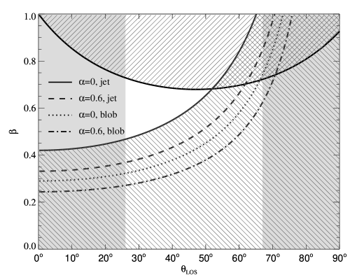
Figure 7: Limit on jet speed $\beta=v/c$ as a function of the angle between a jet and our line of sight, $\theta_{\text{LOS}}$. Upper hatched region: exclusion region from the nondetection of correlated radio–X-ray variability. Lower hatched region: excluded region of the parameter space from jet imaging (Stirling et al., 2001), for a continuous and a clumpy jet, and radio spectral index $\alpha=0$ and $\alpha=0.6$. The grey regions are the current limits on the inclination of the orbit of HDE 226868, and assume that the jet is perpendicular to the orbital plane.

Using the nondetection of correlated variability allows us to set limits on the speed $\beta=v/c$ of the jet and on its inclination. The time for traversing a free jet (with no additional acceleration) is given by $t=d/\beta c$ where $d$ is the distance where the 15 GHz emission is produced and where $\beta$ is the speed of the jet. Simultaneous broadband jet model fits (Markoff et al., 2003) as well as VLBA observations at 8.4 GHz (Stirling et al., 2001) place $d$ in the range of $d\sim 10^{12}$–$10^{14}$ cm. The jet speed is found to be $\beta\sim 0.2$–$0.3$ from broadband analyses (Gallo et al., 2003; Maccarone, 2003), with an upper limit of $\beta\sim 1$ from ballistic ejection events in MQs (e.g., $\Gamma\sim 17$, $\beta\sim 1$, in V4641 Sgr, M. Rupen, priv. comm.). The travel time expected from these numbers is between $10^{12}\,{\text{cm}}/c\approx 33\,\text{s}$ and $10^{14}\,{\text{cm}}/0.2c\approx 4.6\,\text{h}$. Depending on the inclination of the jet, the delay between the X-ray and the radio signals when they reach the observer will be in the same time range. Similar constraints are obtained from VLBA imaging, where we find that for the most probable case of a continuous jet with flat spectrum (Fender et al., 2000) and an angle of the jet with respect to our line of sight, $\theta_{\text{LOS}}\approx$ 35^∘– 40^∘ (Herrero et al., 1995), $\Delta\tau_{\text{max}}$ amounts to $2\cdot 4.2\,\text{h}\approx 8\,\text{h}$. Assuming that at 15 GHz the radio jet of Cyg X-1 has at most the same extent as the 8.7 GHz jet seen by VLBA, Fig. 7 shows that the nondetection of correlated radio–X-ray variability at timescales under 5 hours limits the jet speed to $\beta=0.7$ for a continuous jet with a flat radio spectrum, with a lower limit of $\beta\sim 0.4$, depending on $\theta_{\text{LOS}}$ and consistent with earlier results (Stirling et al., 2001). In the likely case that the 15 GHz jet is smaller than the 8.7 GHz jet, these limits are even tighter.

We conclude that given that no radio–X-ray correlations on minute to hour time scales can be identified and given that correlations on day to month time scales are observed, it is consequent to look for correlations on intermediate time scales like hours to days. Probing these intermediate time scales will be the aim of an approved RXTE observation during 2004.